On Ambiguity in Linear Inverse Problems: Entrywise Bounds on Nearly Data-Consistent Solutions and Entrywise Condition Numbers

This paper concerns the classical and well-studied finite-dimensional linear inverse problem of estimating a true unknown signal vector $\mathbf{x}^{*}\in\mathbb{R}^{N}$ from a noisy data vector $\mathbf{b}\in\mathbb{R}^{M}$ obtained as

where $\mathbf{A}\in\mathbb{R}^{M\times N}$ is the known system matrix and $\mathbf{n}\in\mathbb{R}^{M}$ represents an unknown noise perturbation. In many practical scenarios, this inverse problem is ill-posed, meaning that the original value of $\mathbf{x}^{*}$ might be ambiguous even in the absence of noise, and/or that solutions may be highly sensitive to noise.

While there are many existing theoretical results that characterize ambiguity for this inverse problem, it is frequent to see characterizations phrased in terms of global bounds on the estimation error as a function of the size of the noise [1, 2, 3, 4, 5]. To be concrete, if we let $\hat{\mathbf{x}}$ be the estimate of $\mathbf{x}^{*}$ obtained through some estimation procedure, it is common to see global error bounds of the form

where $\|\cdot\|_{2}$ denotes the standard euclidean norm and the constant $C$ will depend on the characteristics of the estimation procedure, the characteristics of the matrix $\mathbf{A}$, and potentially also the characteristics of the original vector $\mathbf{x}^{*}$ and the data vector $\mathbf{b}$. Examples of this type of bound include:

• •

  If $\mathbf{A}$ has full column rank and $\hat{\mathbf{x}}$ is obtained by least-squares as $\hat{\mathbf{x}}=\mathbf{A}^{\dagger}\mathbf{b}$, then the spectral norm [6, 1, 2, 3, 4, 5] provides the bound

  $$\|\hat{\mathbf{x}}-\mathbf{x}^{*}\|_{2}\leq\sigma_{N}^{-1}(\mathbf{A})\|\mathbf{n}\|_{2},$$

  (3)

  where $\sigma_{i}(\cdot)$ denotes the $i$th largest singular value of a matrix, and $\sigma_{N}^{-1}(\mathbf{A})=\|\mathbf{A}^{\dagger}\|$, where $\|\cdot\|$ denotes the spectral norm and $\mathbf{A}^{\dagger}$ denotes the Moore-Penrose pseudoinverse of $\mathbf{A}$.

• •

  If $\mathbf{A}$ has full column rank and $\hat{\mathbf{x}}$ is obtained by least-squares as $\hat{\mathbf{x}}=\mathbf{A}^{\dagger}\mathbf{b}$, then condition number analysis shows that [1, 2, 3, 4, 5]

  $$\begin{split}&\frac{\|\hat{\mathbf{x}}-\mathbf{x}^{*}\|_{2}}{\|\mathbf{x}^{*}\|_{2}}\leq\kappa(\mathbf{A})\frac{\|\mathbf{n}\|_{2}}{\|\mathbf{b}^{*}\|_{2}},\end{split}$$

  (4)

  where $\mathbf{b}^{*}\triangleq\mathbf{b}-\mathbf{n}$ is the ideal measurement that would have been obtained in the absence of noise,¹¹ 1 Note that the condition number bound that we have presented assumes that $\mathbf{b}^{*}$ belongs to the range of $\mathbf{A}$, which results in a simpler expression than would be obtained otherwise [1, 4, 5]. and $\kappa(\mathbf{A})\triangleq\sigma_{1}(\mathbf{A})/\sigma_{N}(\mathbf{A})$ is the condition number that provides a measure of the sensitivity of the inverse problem to perturbations of the data. The best (smallest) possible condition number is $\kappa(\mathbf{A})=1$, while large values of the condition number imply that even relatively small amounts of noise can lead to potentially large relative errors.

• •

  Many error bounds have been derived that apply under special structural assumptions about $\mathbf{x}^{*}$, such as sparsity [7] or low-rank [8] assumptions. While we make no attempt to be comprehensive, a typical example is the work of Donoho [9], which showed that if $\|\mathbf{n}\|_{2}\leq\varepsilon$ and if $\mathbf{x}^{*}$ is sufficiently sparse, then using $\hat{\mathbf{x}}=\arg\min_{\mathbf{x}\in\mathbb{R}^{N}}\|\mathbf{x}\|_{1}$ subject to $\|\mathbf{A}\mathbf{x}-\mathbf{b}\|_{2}\leq\varepsilon$ will result in a solution that obeys a bound with the same form as Eq. (2) for most large underdetermined matrices $\mathbf{A}$.

We refer to all of these as global bounds because they only provide insight into the aggregate error across all of the entries of the vector $\hat{\mathbf{x}}$, in contrast to an entrywise bound that would provide insight into the potential errors for each of the $N$ individual entries of the vector $\hat{\mathbf{x}}$.

In practical applications, there are many situations where certain entries of $\mathbf{x}^{*}$ are easier to estimate than others and also many situations where certain entries of $\mathbf{x}^{*}$ are more important to estimate accurately. In such situations, global performance bounds can be misleading, and it can be very valuable to know which entries of an obtained solution vector are more trustworthy. For example, this situation occurs frequently in biomedical imaging applications, where the data acquisition procedure can capture more information about certain image voxels than it does for others, leading to spatially-varying ambiguity about the reconstructed image. In such applications, this spatially-varying ambiguity has often previously been evaluated using statistical characterizations like variance maps or Cramér-Rao bounds [10, 11, 12, 13, 14, 15, 16]. Use of such techniques generally requires either explicit modeling of the noise statistics or multiple repetitions of the same data collection procedure to enable empirical variance estimation, and can involve restrictive assumptions about the matrix $\mathbf{A}$ (e.g., that it has full column rank).

In this work, we derive novel tight entrywise bounds that apply to every nearly data-consistent vector $\mathbf{x}$, can be used with arbitrary matrices $\mathbf{A}$ (including rank-deficient matrices), are agnostic to the estimation method used to obtain $\hat{\mathbf{x}}$, and only require knowledge about the size of $\mathbf{n}$ (via an upper bound on $\|\mathbf{n}\|_{2}$) without requiring an accurate statistical model or multiple repetitions of the data collection procedure. To be precise about what we mean by “nearly data-consistent solutions,” we will define $\Gamma_{\varepsilon}(\mathbf{A},\mathbf{b})$ as the set of potential solution vectors $\mathbf{x}$ that are consistent with the data vector $\mathbf{b}$ within a tolerance of $\varepsilon$:

Our theoretical results will provide tight entrywise bounds that must be satisfied by all of the elements of $\Gamma_{\varepsilon}(\mathbf{A},\mathbf{b})$. Notably, if $\|\mathbf{n}\|_{2}\leq\varepsilon$ and data is acquired according to Eq. (1), then the true value $\mathbf{x}^{*}$ must belong to $\Gamma_{\varepsilon}(\mathbf{A},\mathbf{b})$, and our entrywise bounds on $\Gamma_{\varepsilon}(\mathbf{A},\mathbf{b})$ must also be bounds for $\mathbf{x}^{*}$.

Our results (which will be given formally in the sequel as Thm. 1 and its corollaries) will allow us to make useful statements such as: If $\mathbf{x}\in\Gamma_{\varepsilon}(\mathbf{A},\mathbf{b})$, then $x_{i}$, the $i$th entry of $\mathbf{x}$, must belong to a fixed interval $[L_{i},U_{i}]\subset\mathbb{R}$, where the values of $L_{i}$ and $U_{i}$ can be computed explictly based on the values of $\mathbf{A}$, $\mathbf{b}$, $\varepsilon$, and $i$. The values we obtain for $L_{i}$ and $U_{i}$ are also tight in the sense that we can easily identify specific values of $\mathbf{x}\in\Gamma_{\varepsilon}(\mathbf{A},\mathbf{b})$ that achieve the minimal and maximal values of $x_{i}$. We are not aware of existing characterizations of this form, and we believe they enable fundamental new insights into the ambiguities associated with ill-posed inverse problems.

In addition, our results also allow us to define an entrywise condition number $\kappa_{i}(\mathbf{A})$ for the $i$th entry of $\mathbf{x}$. This entrywise condition number (given formally in Corollary 4) will be used in a similar way the condition number $\kappa(\mathbf{A})$ from Eq. (4), but will provide bounds that are generally less pessimistic than Eq. (4) (with $\kappa_{i}(\mathbf{A})\leq\kappa(\mathbf{A}))$ and which explicitly capture the fact that some entries of $\mathbf{x}$ can be substantially better conditioned than others.

During the the final stages of writing this paper, we became aware of mathematical literature involving componentwise condition numbers [17, 18]. Componentwise theory is similar to our proposed entrywise theory in the sense that they both focus on the individual entries of the vector $\mathbf{x}$. However, there are also important differences, including the fact that componentwise theory is frequently used to obtain a single global bound that summarizes the worst-case relative error across all of the individual entries of the vector, while we provide a finer-grained analysis by defining seperate/distinct bounds for each of the $N$ entries of $\mathbf{x}$ individually. In addition, the literature on componentwise theory obtains different results using very different proof techniques compared to what we present in this work.

This paper is organized as follows. We start by introducing some additional notation in Sec. II. This is followed by a presentation of our principal theoretical results in Sec. III. To illustrate the usefulness of our theory, we apply it to characterize an inverse problem from a biomedical imaging application in Sec. IV. We conclude the paper with a discussion of several additional topics in Sec. V, including practical computational considerations for large problem sizes, connections between our proposed bounds and Cramér-Rao bounds under white Gaussian noise assumptions, and interesting potential extensions to common scenarios where additional constraints are available beyond just near data-consistency (e.g., sparsity constraints, low-rank constraints, manifold constraints, etc.).

In addition to the notation that we have already introduced, the following notation is also used throughout the paper. We use $\mathcal{R}(\mathbf{A})$ and $\mathcal{N}(\mathbf{A})$ to respectively denote the range space and nullspace of the matrix $\mathbf{A}$. For a subspace $\mathcal{S}$, we use $\mathcal{S}^{\perp}$ to denote its orthogonal complement, use $\mathbf{P}_{\mathcal{S}}$ to denote its orthogonal projection matrix, and use $\dim(\mathcal{S})$ to denote its dimension.

For a matrix $\mathbf{A}\in\mathbb{R}^{M\times N}$ of rank $r$, we can use the singular value decomposition (SVD) to express $\mathbf{A}$ as $\mathbf{A}=\mathbf{U}\boldsymbol{\Sigma}\mathbf{V}^{T}$, where $\mathbf{U}\in\mathbb{R}^{M\times r}$ and $\mathbf{V}\in\mathbb{R}^{N\times r}$ are matrices with orthonormal columns (corresponding to the left and right singular vectors, respectively), and $\boldsymbol{\Sigma}\in\mathbb{R}^{r\times r}$ is a diagonal matrix with $i$th diagonal element equal to $\sigma_{i}(\mathbf{A})$. The columns of $\mathbf{U}$ form an orthonormal basis for $\mathcal{R}(\mathbf{A})$, while the columns of $\mathbf{V}$ form an orthonormal basis for $\mathcal{R}(\mathbf{A}^{T})$. We can also write the matrix $\mathbf{A}$ using the extended SVD as

where $\mathbf{U}_{\perp}\in\mathbb{R}^{M\times(M-r)}$ and $\mathbf{V}_{\perp}\in\mathbb{R}^{N\times(N-r)}$ are also matrices with orthonormal columns. The columns of $\mathbf{U}_{\perp}$ form an orthonormal basis for $\mathcal{R}^{\perp}(\mathbf{A})=\mathcal{N}(\mathbf{A}^{T})$ and satisfy $\mathbf{U}^{T}\mathbf{U}_{\perp}=\mathbf{0}$, while the columns of $\mathbf{V}_{\perp}$ form an orthonormal basis for $\mathcal{R}^{\perp}(\mathbf{A})=\mathcal{N}(\mathbf{A})$ and satisfy $\mathbf{V}^{T}\mathbf{V}_{\perp}=\mathbf{0}$.

We use $\mathbf{I}_{T}$ to denote the $T\times T$ identity matrix. We denote the Moore-Penrose pseudoinverse of the matrix $\mathbf{A}$ as $\mathbf{A}^{\dagger}=\mathbf{V}\boldsymbol{\Sigma}^{-1}\mathbf{U}^{T}$. If $\mathbf{A}$ is square and nonsingular, then $\mathbf{A}^{\dagger}=\mathbf{A}^{-1}$. If $\mathbf{A}$ has full column rank, then $\mathbf{A}^{\dagger}=(\mathbf{A}^{T}\mathbf{A})^{-1}\mathbf{A}^{T}$. Note that $\mathbf{P}_{\mathcal{R}(\mathbf{A})}=\mathbf{U}\mathbf{U}^{T}=\mathbf{A}\mathbf{A}^{\dagger}$, and that $\mathbf{P}_{\mathcal{R}^{\perp}(\mathbf{A})}=\mathbf{I}_{M}-\mathbf{A}\mathbf{A}^{\dagger}$.

For the positive semidefinite matrix $\mathbf{A}^{T}\mathbf{A}=\mathbf{V}\boldsymbol{\Sigma}^{2}\mathbf{V}^{T}$, we define its square-root as $(\mathbf{A}^{T}\mathbf{A})^{\frac{1}{2}}\triangleq\mathbf{V}\boldsymbol{\Sigma}\mathbf{V}^{T}$.

We will use $\mathbf{e}_{i}\in\mathbb{R}^{N}$ to denote the vector whose $i$th entry is equal to one, with all the other entries equal to zero (i.e., $\mathbf{e}_{i}$ is the $i$th column of $\mathbf{I}_{N}$).

Our main theoretical results are given by the following theorem and its corollaries.

This theorem is valid for arbitrary $\mathbf{A}$, $\mathbf{b}$, and $\varepsilon$, and shows that, depending on how the nullspace of the matrix $\mathbf{A}$ interacts with the vector $\mathbf{e}_{i}$, the value of $x_{i}$ is either restricted to a known interval of length $2\left\|\left(\mathbf{A}^{\dagger}\right)^{T}\mathbf{e}_{i}\right\|_{2}\sqrt{\varepsilon^{2}-\|\mathbf{P}_{\mathcal{R}^{\perp}(\mathbf{A})}\mathbf{b}\|_{2}^{2}}$ or is entirely unconstrained and can be an arbitrary real number.

While Thm. 1 applies to the general case, simplifications occur under assumptions about the rank of $\mathbf{A}$. Specifically:

• •

  If $\mathbf{A}$ has full column rank (i.e., $\mathrm{rank}(\mathbf{A})=N$), then $\mathbf{e}_{i}$ is always orthogonal to $\mathcal{N}(\mathbf{A})$, and $\Phi_{\varepsilon}^{i}(\mathbf{A},\mathbf{b})$ is always a finite interval.

• •

  If $\mathbf{A}$ has full row rank (i.e., $\mathrm{rank}(\mathbf{A})=M$), then $\|\mathbf{P}_{\mathcal{R}^{\perp}(\mathbf{A})}\mathbf{b}\|_{2}$ is always zero. This implies that $\Phi_{\varepsilon}^{i}(\mathbf{A},\mathbf{b})$ is a finite interval of length $2\varepsilon\left\|\left(\mathbf{A}^{\dagger}\right)^{T}\mathbf{e}_{i}\right\|_{2}$ when $\mathbf{e}_{i}$ is orthogonal to $\mathcal{N}(\mathbf{A})$, and is unbounded with $\Phi_{\varepsilon}^{i}(\mathbf{A},\mathbf{b})=\mathbb{R}$ when $\mathbf{e}_{i}$ is not orthogonal to $\mathcal{N}(\mathbf{A})$.

• •

  If $\mathbf{A}$ is square and non-singular (i.e., $\mathrm{rank}(\mathbf{A})=N=M$), then $\Phi_{\varepsilon}^{i}(\mathbf{A},\mathbf{b})$ is always the finite interval of length $2\varepsilon\left\|(\mathbf{A}^{-1})^{T}\mathbf{e}_{i}\right\|_{2}$ with midpoint $\mathbf{e}_{i}^{T}\mathbf{A}^{-1}\mathbf{b}$.

It should also be noted that Thm. 1 will still be valid if the vector $\mathbf{e}_{i}$ is substituted everywhere with an arbitrary nonzero vector $\mathbf{w}\in\mathbb{R}^{N}$. This allows the use of these kinds of bounds in the case where we are potentially interested in the range of values for a weighted linear combination of the entries of $\mathbf{x}$ in the form $\mathbf{w}^{T}\mathbf{x}$. For example, in practical imaging applications, if voxel $x_{i}$ appears to have a larger value than a neighboring voxel $x_{j}$ in the reconstructed image, it may be worthwhile to know tight upper and lower bounds on the value of $x_{i}-x_{j}$ across all $\mathbf{x}\in\Gamma_{\varepsilon}(\mathbf{A},\mathbf{b})$, which would allow direct insight into whether voxel $x_{i}$ is always larger than voxel $x_{j}$ within the class of nearly data-consistent images. This could easily be achieved using the weight vector $\mathbf{w}=\mathbf{e}_{i}-\mathbf{e}_{j}$.

Before giving the proof of Thm. 1, we will first remark that minor manipulations of Thm. 1 also lead to the following corollaries. (As with Thm. 1, these corollaries are also valid if the vector $\mathbf{e}_{i}$ is replaced everywhere with an arbitrary nonzero vector $\mathbf{w}\in\mathbb{R}^{N}$).

Note that Cor. 3 can be viewed an entrywise analogue of the spectral norm bound from Eq. (3). Moreover, Cor. 3 provides a bound that is generally better and never worse than Eq. (3), since we always have that $\left\|\left(\mathbf{A}^{\dagger}\right)^{T}\mathbf{e}_{i}\right\|_{2}\leq\sigma_{N}^{-1}(\mathbf{A})$.

Note that Cor. 4 can be viewed as an entrywise analogue of the condition number bound from Eq. (4). In addition, Cor. 4 provides a bound that is generally better and never worse than Eq. (4), since we always have that $\kappa_{i}(\mathbf{A})\leq\kappa(\mathbf{A})$ (which can be established from the fact that $\left\|\left(\mathbf{A}^{\dagger}\right)^{T}\mathbf{e}_{i}\right\|_{2}\leq\sigma_{N}^{-1}(\mathbf{A})$).

The proof of Thm. 1 is given below.

We illustrate the utility of our new theoretical results by applying them to an example application: image reconstruction in multi-channel magnetic resonance imaging (MRI). Specifically, under the sensitivity encoding model of multi-channel MRI [11, 21], we assume that we are interested in reconstructing a discrete image defined on an $N$-voxel grid, where the value of the image at each voxel is complex-valued. We use $\mathbf{x}\in\mathbb{C}^{N}$ to represent the unknown voxel values. Data measurements are then obtained from this image from a series of $L$ channels, where the data $\mathbf{b}_{\ell}$ from the $\ell$th channel is represented as

where $\mathbf{n}_{\ell}$ represents the noise for the $\ell$th channel, $\mathbf{S}_{\ell}\in\mathbb{C}^{N\times N}$ is a diagonal matrix whose diagonal entries are equal to the corresponding values of the spatially-varying sensitivity profile for the $\ell$th channel, and $\mathbf{F}\in\mathbb{C}^{P\times N}$ represents an operator that performs Fourier transformation followed by some form of sampling. Typically, the sampling rate is chosen to be below the Nyquist rate to allow accelerated data acquisition, resulting in $P<N$. This allows us to represent the inverse problem as

where $\mathbf{b}\in\mathbb{C}^{M}$ is the vertical concatenation of the $\mathbf{b}_{\ell}$ vectors, $\mathbf{n}\in\mathbb{C}^{M}$ is the vertical concatenation of the $\mathbf{n}_{\ell}$ vectors, and $\mathbf{A}\in\mathbb{C}^{M\times N}$ is the vertical concatenation of the $\mathbf{F}\mathbf{S}_{\ell}$ matrices, with $M=LP$.

An important observation is that the matrices and vectors in our example inverse problem are all complex-valued, while our theoretical results are all given assuming the real-valued case. We chose to present our theory for the real-valued case because there exists a standard ordering for real-numbers that enables a simple discussion of lower- and upper-bounds, while the complex-valued case would be much more complicated. However, in order to apply our theory to this scenario, we need to transform the complex-valued problem statement into an equivalent real-valued problem statement. This is easily done by separating each complex-value into its real- and imaginary-components, and then working with an equivalent purely-real expression of the inverse problem (see, e.g., [22, 23]). We have used this real-valued transformation approach in the results that follow. For simplicity and to avoid introducing new notation, we will simply refer to these now real-valued variables using the same notation we used for the complex-valued case (i.e., $\mathbf{x}$, $\mathbf{A}$, $\mathbf{b}$, etc.). From this point forward, all variables should now be interpreted as real-valued.

In our illustrative example application, we use real fully-sampled 32-channel MRI brain data acquired at our institution, which we retrospectively subsample to emulate an accelerated data acquisition procedure as illustrated in Fig. 1, with $P\approx N/3.3$. Note that even though the matrix $\mathbf{F}$ is underdetermined because $P<N$, the overall system $\mathbf{A}$ is still overdetermined because $LP>N$. We have determined numerically that the matrix $\mathbf{A}$ has full column rank.

As can be seen in Fig. 1, our subsampling scheme is designed such that undersampling only occurs along one dimension of the 2D Fourier domain (i.e., the phase encoding dimension in MRI terminology), while the remaining dimension (i.e., the readout dimension in MRI terminology) is fully sampled at the Nyquist rate. This structure implies that one can apply a unitary inverse Fourier transform operator along the fully-sampled readout dimension as a preprocessing step to completely decouple the reconstruction of each image row [24]. Reconstructing each image row independently enables substantial reductions in computational complexity, and the results we present later in this section are all based on this row-decoupled approach.

In our illustrative example, we have used ESPIRiT [25] with circular neighborhoods [26] to estimate the sensitivity profiles needed to form the $\mathbf{S}_{\ell}$ matrices from the fully-sampled central Fourier data. In addition, we incorporate a phase estimate directly into the sensitivity maps so that the reconstructed image will be approximately real-valued [22, 27, 28, 29, 30]. Our formulation also uses prior knowledge of the support of the image and does not estimate voxel locations that are already known to be zero, which is achieved by removing the corresponding columns from the $\mathbf{A}$ matrix [11]. We have also used direct measurements of the multi-channel thermal noise to prewhiten the channels, which allows all thermal noise samples to be treated as independent and identically distributed zero-mean circularly-symmetric complex Gaussian noise [21].

Our illustration will start by calculating the theoretical lower and upper bounds from Thm. 1 for this inverse problem. However, before this can be done, it is important to select an appropriate value of $\varepsilon$. Ideally, the noise perturbation $\mathbf{n}$ in MRI would be purely due to thermal (white Gaussian) noise, such that the distribution of $\|\mathbf{n}\|_{2}$ would follow the chi distribution, which has a well-characterized cumulative distribution function (CDF). If this were the case, then a reasonable approach for selecting $\varepsilon$ might be to choose $\varepsilon$ based on the CDF, e.g., choose $\varepsilon$ so that the probability of observing $\|\mathbf{n}\|_{2}>\varepsilon$ is less than $1\%$. Unfortunately, this approach for determining $\varepsilon$ turns out to be inappropriate for this data, since we observe empircally that we would have $\|\mathbf{P}_{\mathcal{R}^{\perp}(\mathbf{A})}\mathbf{b}\|_{2}>\varepsilon$ under this approach to choosing $\varepsilon$. The reason this approach fails is that we are working with real data, and there are many sources of error in the data beyond just the thermal noise, including minor motion of the human subject during the scan, flow of the subject’s blood and cerebrospinal fluid during the scan, and spin relaxation during the acquisition. All of these contribute to $\mathbf{n}$, causing it to be much larger than would be predicted from the statistics of thermal noise. This example also helps to underscore the point from the introduction that it can be important to have theoretical bounds that are not heavily dependent on statistical noise modeling assumptions, since these assumptions can fail for practical real-world data.

To overcome this practical issue, we have used a heuristic (and likely suboptimal) approach for choosing $\varepsilon$, that is nevertheless good enough for our illustration despite its imperfections. Specifically, we observe that, based on our inverse problem model from Eq. (1), the vector $\mathbf{P}_{\mathcal{R}^{\perp}(\mathbf{A})}\mathbf{b}$ should not contain any of the true signal, and consists entirely of the projection of the noise $\mathbf{n}$ onto the subspace $\mathcal{R}^{\perp}(\mathbf{A})$. If we make the assumption that the noise energy $\mathbf{n}$ distributes relatively evenly across all subspaces of $\mathbb{R}^{M}$ and that $\dim(\mathbb{R}^{M})=M$ and $\dim(\mathcal{R}^{\perp}(\mathbf{A}))=M-N$ are large enough that concentration of measure principles can be applied, then we might reasonably expect that

In what follows, we therefore set $\varepsilon=\sqrt{\frac{M}{M-N}}\|\mathbf{P}_{\mathcal{R}^{\perp}(\mathbf{A})}\mathbf{b}\|_{2}$. Before moving on, we would like to reemphasize that this choice is heuristic and not rigorously justified, and many other ways of choosing $\varepsilon$ could have been used instead. Different choices of $\varepsilon$ would result in a very simple and predictable change in the lower- and upper-bounds $L_{i}$ and $U_{i}$, and would have no effect on other properties that may be of interest such as the entrywise spectral norm-type bound $\|\left(\mathbf{A}^{\dagger}\right)^{T}\mathbf{e}_{i}\|_{2}$ from Cor. 3 or the entrywise condition number $\kappa_{i}(\mathbf{A})$ from Cor. 4.

Figure 2 depicts the entrywise lower- and upper-bounds we obtain on the real- and imaginary-parts of the image based on our choice of $\varepsilon$. In this example, the lower-bounds and upper-bounds are relatively far separated from one another for most voxels of the images, suggesting that near data-consistency constraints themselves may be insufficient to guarantee accurate estimation of the image voxel amplitudes. Of course, it should also be kept in mind that these are worst-case bounds that are independent of any specific image estimation method, and that the practical performance of a specific estimator in the presence of typical (i.e., not worst-case) $\mathbf{n}$ may be better. On the other hand, the fact that there can be this level of variation within the set of near data-consistent images may also encourage an experimenter to consider the use of noise-mitigation strategies so that $\varepsilon$ can be reduced, and/or the redesign of the data acquisition matrix $\mathbf{A}$ so that $\|(\mathbf{A}^{\dagger})^{T}\mathbf{e}_{i}\|_{2}$ can be made smaller.

An important thing to keep in mind is that the spatial maps of $L_{i}$ and $U_{i}$ shown in Fig. 2 may happen to look like realistic MRI images, but they are not themselves elements of $\Gamma_{\varepsilon}(\mathbf{A},\mathbf{b})$. In particular, these maps only provide entrywise bounds, and it is unlikely that these bounds could be achieved by all voxels simultaneously. To illustrate this point, Fig. 3 gives examples of two images belonging to $\Gamma_{\varepsilon}(\mathbf{A},\mathbf{b})$ that achieve the upper- or lower-bounds for specific choices of voxels (using the technique described in the proof of Thm. 1 to identify the extremal cases).

As mentioned in Sec. III, we can also replace $\mathbf{e}_{i}$ in Thm. 1 with a nonzero vector $\mathbf{w}\in\mathbb{R}^{N}$ to construct bounds on linear combinations of the entries of $\mathbf{x}$. We illustrate this point by showing spatial maps of the upper- and lower-bounds on the difference between adjacent voxels ($\mathbf{w}=\mathbf{e}_{i}-\mathbf{e}_{j}$ as discussed in Sec. III, where $\mathbf{e}_{i}$ corresponds to the $i$th voxel position in the image and $\mathbf{e}_{j}$ corresponds to the voxel immediately to the right of the $i$th voxel) in Fig. 4. Interestingly, we observe that there are only a few voxels that are consistently larger or smaller than their neighbors (i.e., the lower-bounds and upper-bounds have consistent sign) within the set of nearly data-consistent solutions.

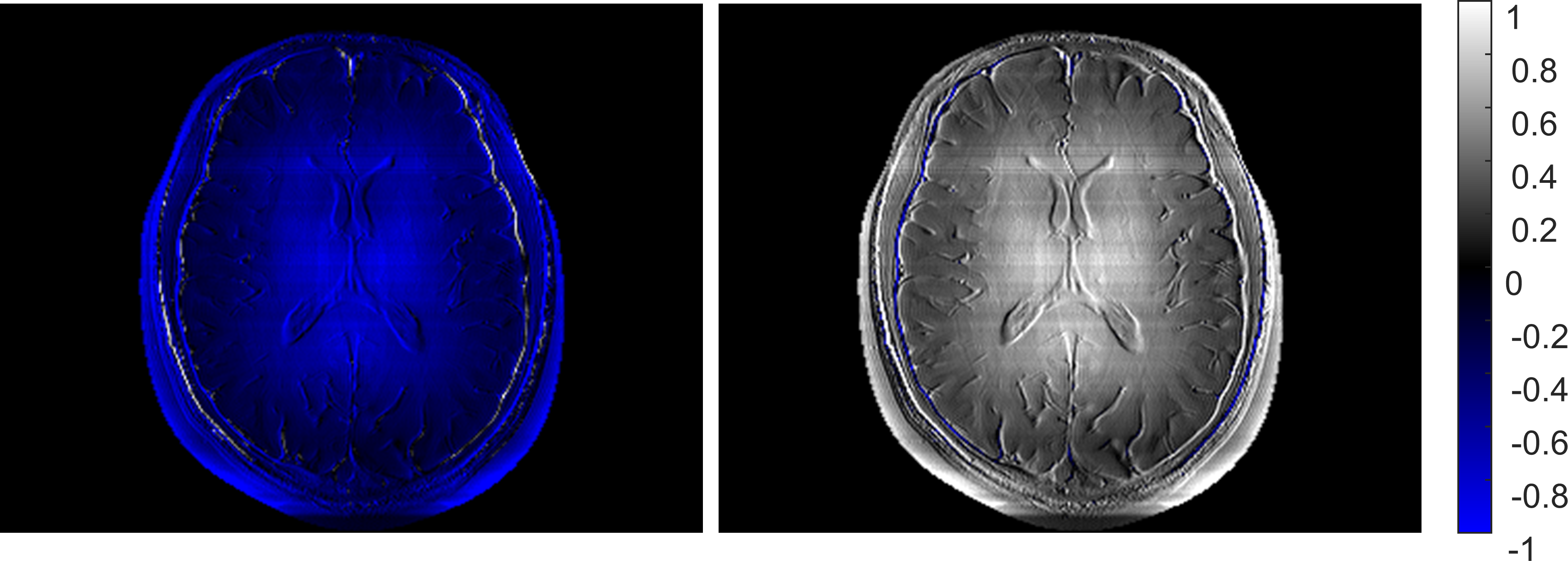
In our final set of illustrations, we compare the global bounds from Eqs. (3) and (4) against our new entrywise bounds from Cors. 3 and 4. Specifically, Fig. 5 focuses on the spectral norm-type bounds from Eq. (3) and Cor. 3, while Fig. 6 focuses on the condition number bounds from Eq. (4) and Cor. 4. In order to show spatial maps of the global bounds in these figures, we have made use of the equivalence of norms on finite dimensional spaces [1, 5]. Specifically, this equivalence implies that

for arbitrary $\mathbf{x}\in\mathbb{R}^{N}$, where $\|\cdot\|_{\infty}$ is the standard infinity norm. This relationship immediately allows a global bound in the form of Eq. (2) to be converted into a bound on the individual elements of $\mathbf{x}$:

which allows us to depict spatial maps of the global bounds.

As can be seen from Figs. 5 and 6, our proposed entrywise bounds are usually better and never worse than the global bounds, consistent with our theoretical expectations. In addition, the entrywise characterizations both do a good job of capturing the fact that the values of certain voxels can be substantially less sensitive to noise perturbations than others, while the traditional global characterizations lack this nuance and are more pessimistic.

References

- [1] G. Golub and C. van Loan, Matrix Computations, 3rd ed. London: The Johns Hopkins University Press, 1996.
- [2] M. Bertero and P. Boccacci, Introduction to Inverse Problems in Imaging. London: Institute of Physics Publishing, 1998.
- [3] T. K. Moon and W. C. Stirling, Mathematical Methods and Algorithms for Signal Processing. Upper Saddle River: Prentice Hall, 2000.
- [4] M. T. Heath, Scientific Computing: An Introductory Survey, 2nd ed. Boston: McGraw-Hill, 2002.
- [5] Y. Bresler, S. Basu, and C. Couvreur, “Hilbert spaces and least squares methods for signal processing,” 2008, unpublished manuscript.
- [6] D. G. Luenberger, Optimization by Vector Space Methods. New York: John Wiley & Sons, 1969.
- [7] E. J. Candès and M. B. Wakin, “An introduction to compressive sampling,” IEEE Signal Process. Mag., vol. 25, pp. 21–30, 2008.
- [8] M. A. Davenport and J. Romberg, “An overview of low-rank matrix recovery from incomplete observations,” IEEE J. Sel. Topics Signal Process., vol. 10, pp. 608–622, 2016.
- [9] D. L. Donoho, “For most large underdetermined systems of equations, the minimal -norm near-solution approximates the sparsest near-solution,” Comm. Pure Appl. Math., vol. 59, pp. 907–934, 2006.
- [10] J. A. Fessler, “Mean and variance of implicitly defined biased estimators (such as penalized maximum likelihood): Applications to tomography,” IEEE Trans. Image Process., vol. 5, pp. 493–506, 1996.
- [11] K. P. Pruessmann, M. Weiger, M. B. Scheidegger, and P. Boesiger, “SENSE: Sensitivity encoding for fast MRI,” Magn. Reson. Med., vol. 42, pp. 952–962, 1999.
- [12] J. Qi and R. M. Leahy, “Resolution and noise properties of MAP reconstruction for fully 3-D PET,” IEEE Trans. Med. Imag., vol. 19, pp. 493–506, 2000.
- [13] J. W. Stayman and J. A. Fessler, “Efficient calculation of resolution and covariance for penalized-likelihood reconstruction in fully 3-D SPECT,” IEEE Trans. Med. Imag., vol. 23, pp. 1543–1555, 2004.
- [14] P. M. Robson, A. K. Grant, A. J. Madhuranthakam, R. Lattanzi, D. K. Sodickson, and C. A. McKenzie, “Comprehensive quantification of signal-to-noise ratio and g-factor for image-based and k-space-based parallel imaging reconstructions,” Magn. Reson. Med., vol. 60, pp. 895–907, 2008.
- [15] S. Ahn and R. M. Leahy, “Analysis of resolution and noise properties of nonquadratically regularized image reconstruction methods for PET,” IEEE Trans. Med. Imag., vol. 27, pp. 413–424, 2008.
- [16] J. P. Haldar and D. Kim, “OEDIPUS: An experiment design framework for sparsity-constrained MRI,” IEEE Trans. Med. Imag., vol. 38, pp. 1545–1558, 2019.
- [17] N. J. Higham, “A survey of componentwise perturbation theory in numerical linear algebra,” in Mathematics of Computation 1943–1993: A Half-Century of Computational Mathematics, W. Gautschi, Ed. Providence: American Mathematical Society, 1994, pp. 49–77.
- [18] F. Cucker, H. Diao, and Y. Wei, “On mixed and componentwise condition numbers for Moore-Penrose inverse and linear least squares problems,” Math. Comput., vol. 76, pp. 947–963, 2007.
- [19] S. Boyd and L. Vandenberghe, Convex Optimization. Cambridge: Cambridge University Press, 2004.
- [20] M. Friendly, G. Monette, and J. Fox, “Elliptical insights: Understanding statistical methods through elliptical geometry,” Stat. Sci., vol. 28, pp. 1–39, 2013.
- [21] K. P. Pruessmann, M. Weiger, P. Börnert, and P. Boesiger, “Advances in sensitivity encoding with arbitrary k-space trajectories,” Magn. Reson. Med., vol. 46, pp. 638–651, 2001.
- [22] M. Bydder and M. D. Robson, “Partial Fourier partially parallel imaging,” Magn. Reson. Med., vol. 53, pp. 1393–1401, 2005.
- [23] T. H. Kim and J. P. Haldar, “Efficient iterative solutions to complex-valued nonlinear least-squares problems with mixed linear and antilinear operators,” Optim. Eng., vol. 23, pp. 749–768, 2022.
- [24] W. E. Kyriakos, L. P. Panych, D. F. Kacher, C.-F. Westin, S. M. Bao, R. V. Mulkern, and F. A. Jolesz, “Sensitivity profiles from an array of coils for encoding and reconstruction in parallel (SPACE-RIP),” Magn. Reson. Med., vol. 44, pp. 301–308, 2000.
- [25] M. Uecker, P. Lai, M. J. Murphy, P. Virtue, M. Elad, J. M. Pauly, S. S. Vasanawala, and M. Lustig, “ESPIRiT – an eigenvalue approach to autocalibrating parallel MRI: Where SENSE meets GRAPPA,” Magn. Reson. Med., vol. 71, pp. 990–1001, 2014.
- [26] R. A. Lobos and J. P. Haldar, “On the shape of convolution kernels in MRI reconstruction: Rectangles versus ellipsoids,” Magn. Reson. Med., vol. 87, pp. 2989–2996, 2022.
- [27] J. D. Willig-Onwuachi, E. N. Yeh, A. K. Grant, M. A. Ohliger, C. A. McKenzie, and D. K. Sodickson, “Phase-constrained parallel MR image reconstruction,” J. Magn. Reson., vol. 176, pp. 187–198, 2005.
- [28] C. Lew, A. R. Pineda, D. Clayton, D. Spielman, F. Chan, and R. Bammer, “SENSE phase-constrained magnitude reconstruction with iterative phase refinement,” Magn. Reson. Med., vol. 58, pp. 910–921, 2007.
- [29] J. P. Haldar, V. J. Wedeen, M. Nezamzadeh, G. Dai, M. W. Weiner, N. Schuff, and Z.-P. Liang, “Improved diffusion imaging through SNR-enhancing joint reconstruction,” Magn. Reson. Med., vol. 69, pp. 277–289, 2013.
- [30] M. Blaimer, M. Heim, D. Neumann, P. M. Jakob, S. Kannengiesser, and F. A. Breuer, “Comparison of phase-constrained parallel MRI approaches: analogies and differences,” Magn. Reson. Med., vol. 75, pp. 1086–1099, 2016.
- [31] L. Landweber, “An iteration formula for Fredholm integral equations of the first kind,” Am. J. Math., vol. 73, pp. 615–624, 1951.
- [32] P. C. Hansen, Rank-Deficient and Discrete Ill-Posed Problems. Philadelphia: SIAM, 1998.
- [33] C. R. Vogel, Computational Methods for Inverse Problems. Philadelphia: SIAM, 2002.
- [34] M. R. Hestenes and E. Stiefel, “Methods of conjugate gradients for solving linear systems,” J. Res. Natl. Bur. Stand., vol. 49, pp. 409–436, 1952.
- [35] C. C. Paige and M. A. Saunders, “LSQR: An algorithm for sparse linear equations and sparse least squares,” ACM Trans. Math. Soft., vol. 8, pp. 43–71, 1982.
- [36] S. M. Kay, Fundamentals of Statistical Signal Processing, Volume I: Estimation Theory. Upper Saddle River: Prentice Hall, 1993.
- [37] F. Pukelsheim, Optimal Design of Experiments. New York: John Wiley & Sons, 1993.
- [38] S. J. Reeves and Z. Zhe, “Sequential algorithms for observation selection,” IEEE Trans. Signal Process., vol. 47, pp. 123–132, 1999.
- [39] D. Xu, M. Jacob, and Z.-P. Liang, “Optimal sampling of k-space with Cartesian grids for parallel MR imaging,” in Proc. Int. Soc. Magn. Reson. Med., 2005, p. 2450.
- [40] J. A. Jones, P. Hodgkinson, A. L. Barker, and P. J. Hore, “Optimal sampling strategies for the measurement of spin-spin relaxation times,” J. Magn. Reson. B, vol. 113, pp. 25–34, 1996.
- [41] G. J. Marseille, M. Fuderer, R. de Beer, A. F. Mehlkopf, and D. van Ormondt, “Reduction of MRI scan time through nonuniform sampling and edge-distribution modeling,” J. Magn. Reson. B, vol. 103, pp. 292–295, 1994.
- [42] S. Cavassila, S. Deval, C. Huegen, D. van Ormondt, and D. Graveron-Demilly, “Cramér-Rao bounds: an evaluation tool for quantitation,” NMR Biomed., vol. 14, pp. 278–283, 2001.
- [43] A. R. Pineda, S. B. Reeder, Z. Wen, and N. J. Pelc, “Cramér-Rao bounds for three-point decomposition of water and fat,” Magn. Reson. Med., vol. 54, pp. 625–635, 2005.
- [44] D. C. Alexander, “A general framework for experiment design in diffusion MRI and its application in measuring direct tissue-microstructure features,” Magn. Reson. Med., vol. 60, pp. 439–448, 2008.
- [45] J. P. Haldar, D. Hernando, and Z.-P. Liang, “Super-resolution reconstruction of MR image sequences with contrast modeling,” in Proc. IEEE Int. Symp. Biomed. Imag., 2009, pp. 266–269.
- [46] D. De Naeyer, Y. De Deene, W. P. Ceelen, P. Segers, and P. Verdonck, “Precision analysis of kinetic modelling estimates in dynamic contrast enhanced MRI,” Magn. Reson. Mater. Phy., vol. 24, pp. 51–66, 2011.
- [47] B. Zhao, J. P. Haldar, C. Liao, D. Ma, Y. Jiang, M. A. Griswold, K. Setsompop, and L. L. Wald, “Optimal experiment design for magnetic resonance fingerprinting: Cramer-Rao bound meets spin dynamics,” IEEE Trans. Med. Imag., vol. 81, pp. 1620–1633, 2019.
- [48] M. Lustig, D. Donoho, and J. M. Pauly, “Sparse MRI: The application of compressed sensing for rapid MR imaging,” Magn. Reson. Med., vol. 58, pp. 1182–1195, 2007.
- [49] K. T. Block, M. Uecker, and J. Frahm, “Undersampled radial MRI with multiple coils. iterative image reconstruction using a total variation constraint.” Magn. Reson. Med., vol. 57, pp. 1086–1098, 2007.
- [50] J. Trzasko and A. Manduca, “Highly undersampled magnetic resonance image reconstruction via homotopic -minimization,” IEEE Trans. Med. Imag., vol. 28, pp. 106–121, 2009.
- [51] H. Jung, K. Sung, K. S. Nayak, E. Y. Kim, and J. C. Ye, “k-t FOCUSS: A general compressed sensing framework for high resolution dynamic MRI,” Magn. Reson. Med., vol. 61, pp. 103–116, 2009.
- [52] J. P. Haldar, D. Hernando, and Z.-P. Liang, “Compressed-sensing MRI with random encoding,” IEEE Trans. Med. Imag., vol. 30, pp. 893–903, 2011.
- [53] Z.-P. Liang, “Spatiotemporal imaging with partially separable functions,” in Proc. IEEE Int. Symp. Biomed. Imag., 2007, pp. 988–991.
- [54] J. P. Haldar and Z.-P. Liang, “Spatiotemporal imaging with partially separable functions: A matrix recovery approach,” in Proc. IEEE Int. Symp. Biomed. Imag., 2010, pp. 716–719.
- [55] S. G. Lingala, Y. Hu, E. DiBella, and M. Jacob, “Accelerated dynamic MRI exploiting sparsity and low-rank structure: k-t SLR,” IEEE Trans. Med. Imag., vol. 30, pp. 1042–1054, 2011.
- [56] B. Zhao, J. P. Haldar, A. G. Christodoulou, and Z.-P. Liang, “Image reconstruction from highly undersampled -space data with joint partial separability and sparsity constraints,” IEEE Trans. Med. Imag., vol. 31, pp. 1809–1820, 2012.
- [57] J. Trzasko and A. Manduca, “Local versus global low-rank promotion in dynamic MRI series reconstruction,” in Proc. Int. Soc. Magn. Reson. Med., 2011, p. 4371.
- [58] R. Otazo, E. Candès, and D. K. Sodickson, “Low-rank plus sparse matrix decomposition for accelerated dynamic MRI with separation of background and dynamic components,” Magn. Reson. Med., vol. 73, pp. 1125–1136, 2015.
- [59] J. P. Haldar and K. Setsompop, “Linear predictability in magnetic resonance imaging reconstruction: Leveraging shift-invariant Fourier structure for faster and better imaging,” IEEE Signal Process. Mag., vol. 37, pp. 69–82, 2020.
- [60] P. J. Shin, P. E. Z. Larson, M. A. Ohliger, M. Elad, J. M. Pauly, D. B. Vigneron, and M. Lustig, “Calibrationless parallel imaging reconstruction based on structured low-rank matrix completion,” Magn. Reson. Med., vol. 72, pp. 959–970, 2014.
- [61] J. P. Haldar, “Low-rank modeling of local -space neighborhoods (LORAKS) for constrained MRI,” IEEE Trans. Med. Imag., vol. 33, pp. 668–681, 2014.
- [62] K. H. Jin, D. Lee, and J. C. Ye, “A general framework for compressed sensing and parallel MRI using annihilating filter based low-rank Hankel matrix,” IEEE Trans. Comput. Imaging, vol. 2, pp. 480–495, 2016.
- [63] G. Ongie and M. Jacob, “Off-the-grid recovery of piecewise constant images from few Fourier samples,” SIAM J. Imaging Sci., vol. 9, pp. 1004–1041, 2016.
- [64] F. Knoll, K. Hammernik, C. Zhang, S. Moeller, T. Pock, D. K. Sodickson, and M. Akcakaya, “Deep-learning methods for parallel magnetic resonance imaging reconstruction: A survey of the current approaches, trends, and issues,” IEEE Signal Process. Mag., vol. 37, pp. 128–140, 2020.
- [65] D. Liang, J. Cheng, Z. Ke, and L. Ying, “Deep magnetic resonance imaging reconstruction: Inverse problems meet neural networks,” IEEE Signal Process. Mag., vol. 37, pp. 141–151, 2020.
- [66] C. M. Sandino, J. Y. Cheng, F. Chen, M. Mardani, J. M. Pauly, and S. S. Vasanawala, “Compressed sensing: From research to clinical practice with deep neural networks,” IEEE Signal Process. Mag., vol. 37, pp. 117–127, 2020.
- [67] Z.-P. Liang, F. Boada, T. Constable, E. M. Haacke, P. C. Lauterbur, and M. R. Smith, “Constrained reconstruction methods in MR imaging,” Rev. Magn. Reson. Med., vol. 4, pp. 67–185, 1992.
- [68] J. P. Haldar and Z.-P. Liang, ““Early” constrained reconstruction methods,” in Magnetic Resonance Image Reconstruction: Theory, Methods, and Applications, M. Doneva, M. Akcakaya, and C. Prieto, Eds. London: Academic Press, 2022, ch. 5, pp. 105–125.
- [69] V. Antun, F. Renna, C. Poon, B. Adcock, and A. C. Hansen, “On instabilities of deep learning in image reconstruction and the potential costs of AI,” Proc. Natl. Acad. Sci. USA, vol. 117, pp. 30 088–30 095, 2020.
- [70] C.-C. Chan and J. P. Haldar, “Local perturbation responses and checkerboard tests: Characterization tools for nonlinear MRI methods,” Magn. Reson. Med., vol. 86, pp. 1873–1887, 2021.