Post-inflationary axions: a minimal target for axion haloscopes
Marco Gorghettoa and Edward Hardyb
a
Department of Particle Physics and Astrophysics, Weizmann Institute of Science,
Herzl St 234, Rehovot 761001, Israel
b Department of Mathematical Sciences, University of Liverpool,
Liverpool, L69 7ZL, United Kingdom
An axion-like-particle (ALP) in the post-inflationary scenario with domain wall number can be dark matter if the residual symmetry has a small explicit breaking. Although we cannot determine the full dynamics of the system reliably, we provide evidence that such an ALP can account for the observed dark matter abundance while having a relatively small decay constant and consequently a possibly large coupling to photons. In particular, we determine the number of domain walls per Hubble patch around the time when they form using numerical simulations and combine this with analytic expectations about the subsequent dynamics. We show that the strongest constraint on the decay constant is likely to come from the dark matter ALPs being produced with large isocurvature fluctuations at small spatial scales. We also comment on the uncertainties on the dark matter small-scale structure that might form from these overdensities, in particular pointing out the importance of quantum pressure in the case.
1 Introduction
By virtue of being the most robust known solution to the strong CP problem, the QCD axion is one of the best-motivated extensions to the Standard Model (SM) [1, 2, 3, 4, 5, 6, 7]. It is also plausible that one or more axion-like-particles (ALPs), i.e. pseudo-Nambu-Goldstone bosons of spontaneously broken approximate global U(1) symmetries, exist (we will use the name ‘axion’ to refer to both ALPs and QCD axions). For instance, current understanding suggests that axions might be common in many string theory constructions [8, 9, 10, 11, 12]. Additionally, axions are good candidates to be dark matter (DM) [13, 14, 15]: for masses and typical interaction strengths, they are stable on cosmological timescales [16, 17], and a nonrelativistic relic population is inevitably produced in the early Universe.
Motivated by these appealing features, numerous axion dark matter detection experiments have been proposed targetting different ranges of axion masses [18, 19, 20]. Many of these rely on the axion having a coupling to photons
| (1) |
where is the axion, is the electromagnetic field strength, is its dual, and is the axion-to-photon coupling constant. For the QCD axion this coupling is
| (2) | ||||
where is the axion decay constant and is the fine-structure constant, and the second line follows from the fixed relation between the QCD axion mass and decay constant. and are the anomaly coefficients of the Peccei-Quinn (PQ) symmetry with respect to electromagnetism and QCD respectively [21, 22, 23]. Meanwhile, the term in eq. (2) that is independent of comes from the mixing of the axion with the neutral pion, ultimately due to the PQ anomaly with respect to QCD and the fact that quarks are charged. Unless is very large, the couplings in eq. (2) are challenging to reach experimentally.11 1 See however e.g. [24, 25, 26] for ways the QCD axion coupling to photons can be enhanced. This difficulty motivates understanding the plausible values of the axion-to-photon coupling in other theories that are more general than the QCD axion but which might not solve the strong-CP problem.
An ALP’s coupling to photons does not get a contribution analogous to the constant part in eq. (2) (because the U(1) symmetry that gives rise to it is not anomalous under QCD) so might simply vanish. Nevertheless, it is possible that the new physics associated to the ALP carries an anomaly with respect to electromagnetism, so could plausibly be non-zero. Similarly to eq. (2), we parametrise such a coupling by
| (3) |
In minimal theories and are determined by the anomaly coefficients of the U(1) symmetry with respect to QED and a new confining gauge group, and in many concrete models . For convenience we further define the UV model-independent ‘coupling’ ; the relation between this and the true coupling depends on the underlying theory. Unlike the QCD axion, an ALP’s decay constant is independent of its mass. As a result, for fixed values of the mass and , the axion-to-photon coupling can be large if is small enough. However, if the axion is to comprise the full dark matter abundance in a standard cosmological history, has a lower bound, ultimately because the energy density in the axion field available to produce dark matter is proportional to .
There are two broad axion cosmological scenarios (see [27, 28] for an intermediate regime). In the pre-inflationary scenario the global symmetry that gives rise to the axion is broken during inflation and is never subsequently restored. In this case, the axion field initially takes a constant value over the observable Universe, and the axion relic abundance is produced by the misalignment mechanism. If the ALP’s mass is temperature-independent
| (4) |
where is the observed DM abundance, is the initial misalignment angle, and is a function that accounts for anharmonicities in the axion potential. For typical axion potentials for and increases slowly as approaches . Constraints on the size of primordial isocurvature perturbations give a lower bound on that depends on the Hubble scale during inflation, see Appendix A. For instance, for a cosine potential increases only logarithmically with , and requires which gives . From eq. (4), if the axion-to-photon coupling is constrained to be 22 2 An ALP’s misalignment relic abundance, and consequently the maximum , can be larger if the axion mass is temperature dependent. This is also possible in theories with multiple axions [29], different cosmological histories, and different axion potentials [30].
| (5) |
In the post-inflationary scenario the symmetry is instead unbroken at the end of inflation or is subsequently restored e.g. by finite temperature effects. As a result, the field is initially inhomogeneous over our observable Hubble patch and the axion relic abundance is determined by the decay of a network of topological defects: global cosmic strings and domain walls. In this paper, we argue that an ALP in the post-inflationary scenario can be all the DM with a much smaller (i.e., for fixed , a larger coupling to photons) than in the pre-inflationary scenario while being compatible with observational constraints, the most important of which is expected to come from bounds on primordial isocurvature perturbations.33 3 A related analysis of the same theory can be found in [31, 32] focusing on the gravitational waves from domain walls, see also [33] for a similar study of a different theory that has an axion. This is possible because, if , the string-domain wall network might be long-lived, which results in the dark matter produced by its decay being redshifted less. We also analyse the impact of the isocurvature constraints on possible gravitational wave signals from topological defects and discuss the properties of, and the uncertainties in, the dark matter substructure that might form in the early Universe.
We stress that it is difficult to analyse the system’s dynamics from first principles because they are both non-linear and involve large scale separations, and as a result the field evolution is presently unknown. Nevertheless, we make progress by combing results from numerical simulations with reasonable standard assumptions about the dynamics of the domain wall network (which we can only very partially check). In particular, in Section 3 we determine number of domain walls per Hubble patch at the time when the axion mass becomes cosmologically relevant (when the Hubble parameter is ), which is important for the resulting dark matter abundance, and provide evidence that the axions emitted from the string-domain wall system are, at most, mildly relativistic. Our results for , applicable for both ALPs and the QCD axion, suggest that this quantity increases logarithmically with , and mean that an extrapolation of simulation results is needed. We also discuss the numerous remaining uncertainties on the evolution of after this time, and on the spatial distribution of the axions produced from the string-domain wall system.
The structure of the paper is as follows. In Section 2 we introduce the post-inflationary scenario for ALPs and discuss analytic expectations about the dynamics and the dark matter relic abundance, and in Section 3 we present results from numerical simulations of the string-wall system. In Section 4 we analyse the observational constraints on the theory and discuss its relevance for upcoming axion dark matter searches, and we also comment on the possible gravitational waves signals and dark matter substructure. In Section 5 we describe future directions and extensions.
2 Early universe evolution
An axion-like-particle (ALP) is the pseudo-Nambu Goldstone boson, , of an approximate global U(1) symmetry that is spontaneously broken at a high scale . Because is an angular variable, the theory preserves an exact discrete shift symmetry . The simplest model in which this happens consists of a complex scalar with an approximate global U(1) symmetry and potential
| (6) |
that induces a vacuum expectation value . Expanding , the axion is a Goldstone mode, while the radial mode has (large) mass , which is often of order .
We assume that the U(1) symmetry is broken by non-perturbative effects, e.g. because it is anomalous with respect to a new confining gauge group. Such a breaking leads to a potential for that is invariant under . In general and are related by , where has to be an integer otherwise the symmetry would be violated (in KSVZ-like models, is the number of fermions charged under U(1)). As a result, the potential induced by a particular non-perturbative contribution does not necessarily break the U(1) symmetry completely, and can leave a subgroup unbroken. For instance, the total axion potential might be
| (7) |
where the first term comes from the non-perturbative contribution.
In eq. (7), represents additional sources of U(1) breaking that violate the discrete symmetry while still preserving . Such breaking is expected because it is believed that there are no exact global symmetries in quantum gravity [34, 35, 36] (implications for the QCD axion have been studied in e.g. [37, 38, 39, 40, 41, 42, 43, 44, 45, 46]).44 4 This happens e.g. via higher dimensional operators of dimension of the form , where is the Planck Mass and . If , needs to be large in order for the U(1) to be an approximate symmetry. On the other hand, if is exponentially suppressed (as expected from some non-perturbative gravitational processes such as wormholes [34, 35]) can be small. As an example, although the particular form does not matter, one can consider
| (8) |
with . In the absence of there would be inequivalent degenerate vacua, but the energy densities of these vacua are shifted by due to by . We demand so that the global minimum of the full potential is a perturbation of one of the preserving minima and the axion mass is dominated by the first term in eq. (7) [47]. In the following we will take , but this choice will not have any effect.
The equations of motion (EoM) from the potentials in eqs. (6) and (7) admit topologically non-trivial field configurations called strings and domain walls respectively [48, 49, 50, 51] (see [52] for a review). These form if the field is inhomogeneous, as is the case in the post-inflationary scenario. We assume a standard cosmological history, and, as we discuss subsequently, in all theories of interest the strings and domain walls are destroyed before matter-radiation equality (MRE). During the preceding era of radiation domination the Hubble parameter is , where is the scale factor of the Universe and is the cosmic time. Unless otherwise stated we assume that the axion potential is independent of the temperature of the Universe.
2.1 The scaling regime
After the PQ symmetry spontaneously breaks, has initially random spatial fluctuations. The axion potential in eq. (7) is cosmologically irrelevant while so a network of cosmic strings forms. The strings occur in regions of space in which the axion U(1) is wrapped non-trivially, and they have (evolving) energy per unit length, i.e. tension,
| (9) |
The string network is driven to an attractor, scaling, solution on which there is approximately one Hubble length of string per Hubble volume. To study this regime, numerical simulations of the nonlinear EoM from the potential in eq. (6) are required and an extrapolation in is needed. In particular, simulations can only be carried out with a relatively small value of so the scale separation between the string thickness (of order ) and the Hubble distance is far from the values relevant shortly before [53].
We define the number of strings per Hubble volume where is the length of string in a volume . Simulations show that during the scaling regime has a logarithmic increase, . The energy density in (long) strings is, from eq. (9), and the network releases energy density into (relativistic) axion waves at a rate . Additionally, simulations suggest that at the relevant large most of the axions are emitted with momentum of order Hubble. The resulting axion number density released until time is given by , which is dominantly produced in the final few Hubble times prior to , see Appendix B.55 5 See however [54] which suggests a scale invariant instantaneous emission spectrum, which would reduce the relic abundance by a factor of relative to eq. (10).
The scaling regime continues until the time when the Hubble parameter equals the axion mass, , when the first (-preserving) contribution to the axion potential in eq. (7) starts to be cosmologically relevant. We indicate quantities at that moment by , e.g. is the Hubble parameter at this time, and we define , which is of for the that we will consider.
The axion waves emitted by strings prior to become nonrelativistic after and contribute to the dark matter relic abundance, see Section 4.1 of [55] and [56] for more details. Evaluating at and redshifting to today, the resulting dark matter from strings during the scaling regime, , is, for a temperature-independent ,
| (10) |
For the axion masses and decay constants of interest, and , we have . Therefore, assuming that the logarithmic growth in is valid also for , (if take a different value the abundance can be calculated accordingly from eq. (10)). Note that for larger values of or , the axion number density is substantially reduced between the time when the axions are relativistic and when they become nonrelativistic, because the amplitude of the axion field is much larger than and nonlinear effects from the axion potential become relevant. As a result, the abundance decreases with respect to eq. (10), see [55]. For the effect is of order 1, comparable to the other uncertainties in eq. (10).66 6 The non-linear evolution is more important for the QCD axion because has a strong temperature dependence [56].
2.2 The expected post-inflationary relic abundance
Once the axion potential is relevant at , domain walls form, across which the axion field interpolates between vacua. Each string is bounded by domain walls. The domain walls have a tension, i.e. energy per unit area, given by , where is a numerical factor ( for a cosine and is similar for other typical potentials).
If the domain walls connect the same vacuum of the potential in eq. (7), , and the string and domain wall network is unstable and expected to decay. In the process axion waves are emitted, and subsequently the axion field oscillates around the global minimum of its potential and behaves as dark matter. The contribution to the axion abundance produced by the domain walls and strings at this time is hard to determine reliably. If the network is destroyed soon after , it might be relatively unimportant compared to that from the scaling regime, in eq. (10), because the energy in strings is enhanced relative to that in domain walls by the logarithmically boosted string tension (see eq. (14) below). Including only the contribution from the scaling regime, the value of for which an post-inflationary ALP makes up all the DM is of same order as that in the pre-inflationary scenario with an initial misalignment angle close to the top of the potential, see eq. (5) and Figure 4. We do however stress that eq. (10) is a lower bound on the axion relic abundance; the domain wall network might take longer to decay than expected, in which case it could produce a sizable additional contribution resulting in smaller required .
In contrast, if the domain walls interpolate between the inequivalent vacua of the first term in eq. (7). In the absence of they would form a topologically stable network after [51] which would come to dominate the energy density in the Universe [57]. However, the energy bias between the vacua induced by is believed to lead to the destruction of the network when becomes cosmologically relevant [51, 58, 59, 60]. This is thought to happen when the energy density in domain walls, , is approximately equal to the energy density provided by the bias term, , i.e. the Hubble parameter when the network is destroyed is . The energy released by the domain walls is expected (but not proven) to dominantly go into dark matter axions, with a small fraction emitted as gravitational waves [31].
If , the energy density difference between the local minima is of and the symmetry is badly broken. As a result, the evolution of the string-domain wall network, and the axion relic abundance, is likely to be similar to that in the scenario. However, if the domain wall network is long-lived and is destroyed when the Hubble parameter is . Unfortunately, the dynamics in this case are even harder to study with numerical simulations than the scenario. This is because there is another relevant scale, , so a second extrapolation, in , is needed. Simulations can only reach values , whereas we will see in Section 4.1 that values up to (determined by ) are possible. The too-small are an issue not only because the string tension depends on this factor, but also because the string dynamics are dominated by emission of high energy modes with energy of order for [56]. The second extrapolation is perhaps even more problematic because, as increases, there is a growing mismatch between the typical spatial size of the domain walls, which extend over an Hubble length , and the frequency of the axions they are expected to emit (of order ). It is plausible that this could e.g. decrease the ability of the domain walls to radiate axions as increases, which might even qualitatively change the properties of the network when .
Nevertheless, we proceed with some standard analytic expectations, which we will subsequently partially check. It is useful to define the domain-wall area per Hubble patch , where is the total domain wall area in a volume . measures parametrically the total area of domain walls in one Hubble patch in units of the Hubble area , so the energy density in domain walls is
| (11) |
While is cosmologically irrelevant, at the domain walls are thought to survive in a domain wall ‘scaling regime’: is expected to be approximately constant in time, and likely not far from [61] (or slightly larger, because of the logarithmic violation discussed in Section 3). To maintain this, the network must emit energy density at a rate
| (12) |
i.e. an energy density of order is released every Hubble time.77 7 This is because , where is the energy density of a system of domain walls that coincides with that in the scaling regime at , but evolves freely, i.e. the domain walls are fixed in comoving coordinates. The momentum of the axions produced is unknown and could be set by either of the two scales relevant to the domain walls: their size or their thickness . Although the latter is suggested by results of simulations at small and , see Section 3, it is not clear whether this remains the case for physical parameters. Regardless of this uncertainty, because the emitted energy dominantly goes into at most semi-relativistic modes, the axion number density produced until time is approximately , i.e.
| (13) | ||||
| (14) |
where is the scale factor. Because , it is clear from eq. (13) that the number density is mostly produced at the latest times that the network survives to and is dominated by the axions emitted during the Hubble time immediately preceding the domain wall network’s destruction. If the network survives up to , the axion number density is parametrically enhanced, by a factor , with respect to that from misalignment, which is at , see eq. (14).
At , all the domain walls are destroyed and their energy density is released, where denotes the value of at this time. The resulting axion number density is similar that left from the evolution of domain walls up to , calculated in eq. (14). Therefore, the axion relic abundance from energy stored in domain walls is approximately
| (15) | ||||
where we set in the second line. For this contribution far exceeds that produced by strings before given in eq. (10). Moreover, in Appendix C we show that the abundance produced from energy in strings after is in turn smaller than that released by strings before (fundamentally because and therefore decrease faster than and as increases). Therefore we expect that eq. (15) approximates the total relic abundance in this scenario.
If (i.e. is small enough), an axion in the post-inflationary scenario with can account for the full dark matter abundance with smaller than in the post-inflationary and the pre-inflationary scenario for any value of compatible with isocurvature constraints. The possible coupling of such an axion with to photons is correspondingly enhanced, in particular
| (16) |
As mentioned, we expect , but we keep eq. (16) in terms of because we do not have a reliable way of predicting the relation between and .
2.3 The density power spectrum
The number of strings and domain walls per Hubble patch varies by order one factors between different Hubble patches. Therefore, immediately after the decay of the string-wall network (when most of the axions are expected to be produced), the energy density of the axion field is expected to be left with substantial inhomogeneities over Hubble distances. Being only in the axion energy density, these are isocurvature fluctuations. Their properties are conveniently described by the power spectrum of the overdensity field , where is the non-relativistic energy density of the axion when the field is close to its minimum, is its spatial average, and we defined
| (17) |
for a generic field with Fourier transform . Unfortunately the power spectrum of a post-inflationary ALP is not known; below we summarise its possible form based on analytical arguments and hints from numerical simulations.
If , the network decays at and therefore the resulting fluctuations are likely to be on comoving scales approximately set by . Numerical simulations at small scale separation, , support this picture, with peaked (and obtaining an value) at comoving momenta [62, 63, 55]. (This corresponds to of order one at spatial scales approximately set by , with .) At larger comoving scales, , the perturbations are uncorrelated, by causality. From eq. (17), this fixes the spectrum to have the ‘white-noise’ form for , where is a numerical constant. The axion waves are expected to be produced marginally relativistic (with momentum , i.e. wavelength coinciding with the typical size of the strings and domain walls – which might also be connected to the density spectrum being peaked at ). Therefore they initially free stream over comoving distances . This might partly wash out the order-one fluctuations, but should leave the IR () part of the spectrum largely unchanged because the axions will not free-stream over the corresponding distances [63]. In Figure 1 we show a sketch of the anticipated power spectrum.
If the spatial distribution of domain walls is expected to lead to order one fluctuations in the axion energy density immediately after the network’s destruction. Although not yet established with simulations, it is plausible that these will be on scales set parametrically by , where will be correspondingly peaked, i.e. on comoving spatial scales that are larger than . Similarly to the case, at the spectrum acquires a white-noise form
| (18) |
where is an undetermined constant, possibly not far from order one. As discussed in the previous Section, the axion momentum distribution is uncertain in this scenario. If axions are dominantly produced with momentum , they are initially highly non-relativistic for and their free-streaming will be irrelevant. However, if they are produced with momentum , they are initially semi-relativistic and will free-stream over comoving distances of order .88 8 More precisely, if produced with momentum the axions would free-stream a comoving distance where is the cosmic time at matter-radiation equality [64]. Similarly to the scenario, fluctuations on comoving scales will be affected, but the part of (which is what will be relevant to the constraints that we discuss shortly) is expected to be left unchanged. Unfortunately, the reach in and in simulations is not sufficient for us to extrapolate to obtain the value of with the physical parameters and the details of the peak of are especially uncertain.
3 Comparison with numerical results
3.1 The area parameter
The area parameters and entering in the abundance of eq. (15) can be extracted from numerical simulations of eqs. (6) and (7), although these have to be extrapolated in and, for , also . More precisely, we define to be the area of the surfaces where the axion is at the maxima of the -preserving potential in eq. (7), , , which correspond to domain walls when . Details of the simulations and additional results may be found in Appendix C.
Figure 2 (left) shows the evolution of with , i.e. during the string scaling regime, with time parametrised by . In this era is proportional to , so we plot . Results are given for both the so-called ‘fat’ string system (in which in eq. (6)) and the physical system (in which is constant), with initial conditions close to the attractor solution.99 9 The fat string system displays better numerical properties. For instance, because more cosmic time is available between two fixed values of , this system reaches the attractor solution faster. Not surprisingly given the logarithmic increase of on the attractor, grows with . For the fat string system is approximately proportional to ; this can be seen from the plot of in Figure 5 in Appendix C.2. The results for for the physical system are less clear but are compatible with this ratio approaching a constant value. This possibility is supported by the fact that is automatic if the average string curvature is proportional to the Hubble parameter, as is expected by causality during the scaling regime. On the other hand, even for the fat string system, the uncertainty on is still large enough that we cannot exclude a deviation at much later times, .
Given that during the scaling regime is well fitted by a linear function of [56], a natural ansatz for is
| (19) |
where the last two terms encode possible deviations from linearity that are irrelevant at late times, but affect the evolution at the small times (i.e. s) that are accessible to simulations. This form fits the fat string data well with . It also fits the physical data well, however the value of is more uncertain and we estimate , see Appendix C.2 (a quadratic dependence on also gives an acceptable fit to both and for the physical system, see also [56]). Therefore, at the physically relevant for an ALP (for in the range , c.f. Figure 4), the area parameter is likely to be . Meanwhile, given the relation between and , for the QCD axion . As a result, a linear extrapolation predicts in this case (a quadratic extrapolation would instead give ). Similarly to , these values of are much larger than the values that occur at small scale separations.
In Figure 2 (right) we show the effect of the -preserving axion potential in eq. (7) with . In particular, we plot the evolution of for the fat system for different choices of the axion mass , which we parametrise by , with time represented by . To allow for a larger dynamical range, is also taken to be proportional to , so that the ratio is constant. (Although this is not physical, we expect the qualitative features of the dynamics to be similar, like in the fat string system.) For comparison, we also show the results obtained without any axion potential, (dashed lines, which correspond to the evolution in Figure 2, left). We plot the data starting from , by which time strings are cleanly-defined objects. Note that the simulated values of are much smaller than the physically relevant ones. The results indicate that at the logarithmic growth of stops. Not surprisingly, the increase in the area of the surfaces where with translates into a larger number of domain walls at this time (at least for the parameters possible in simulations) and the relation remains approximately true.1010 10 As shown in Figure 3 of Appendix C.2, the growth of continues unaffected slightly longer.
Figure 2 (right) also shows a hint that might decrease at large in the simulations with larger . Although tentative, such a change is plausible and could indicate the domain walls, rather than the strings, starting to dominate the dynamics of the system (as might be expected once ). Unfortunately, we do not have sufficient numerical reach to determine the asymptotic behaviour, e.g. it might be that the system is drawn to a new attractor with independent of but we cannot determine whether this is the case. We also cannot rule out more dramatic qualitative changes in the network’s dynamics at and . Additionally, the non-linear transient of the waves produced during the scaling regime (expected to happen when ) could affect the evolution of the domain walls around the time when in a way that we do not have control of in both the case of an ALP and especially the QCD axion.
Given these multiple complicating factors, we have little control on the physically relevant value of , and thus leave it unfixed in what follows. The resulting uncertainty on and is slightly tempered by the square-root in eq. (16).
3.2 The emission spectrum
As discussed above eq. (13), the momentum of the axions emitted by the string-domain wall network is important for the axion relic abundance. The momentum distribution is encoded into the energy spectrum , which can be extracted from numerical simulations as described in Appendix C. However, while domain walls are present they contaminate the axion field (and because they have thickness they cannot be easily masked). Instead, it is more convenient to carry out simulations with non-zero breaking parameter, and extract the axion energy spectrum after all the domain walls are destroyed. However, we stress that we can only determine the evolution and the spectrum at very unphysical values of and , and the true emission spectrum could differ from simulation results dramatically.
In Figure 3 (left) we plot as a function of time in such simulations for the fat string-domain wall system with different amounts of breaking, which we parameterise by where is defined in eq. (8). We fix (i.e. ) and . As expected, larger results in the network being destroyed earlier.1111 11 We do not attempt to fit a relation between the and the Hubble parameter when the network is destroyed , which would require extremely careful extrapolations in and . In Figure 3 (right) we plot the axion energy spectrum at the end of the simulations shown in the left panel, by which time all the strings and domain walls are destroyed, the axion field amplitude is over all of space (apart from a few oscillons [62], which contain a negligible fraction of the axion energy density), and the spectrum has reached a fixed shape. Because of the fat strings and domain walls, axions produced with proper momentum or (the latter corresponding to the string core scale) always have, and remain at, the same comoving momentum or respectively. At the values of that can be simulated, the strings are expected to emit energy dominantly to axions with UV momentum [53, 56] although this has only been shown with .
In Figure 3 (right), the axion energy spectrum increases as , and therefore , decreases. This indicates that, at least for the smallest , a sizable fraction of the energy density in axion waves is coming from the domain walls (because the relic abundance from strings is dominantly produced at rather than later). Although only gives a mild separation between and , Figure 3 suggests that with longer lived domain walls an increased fraction of the axion waves are produced at most borderline rather that ultra-relativistic, with physical momenta rather than (or equivalently, comoving momentum rather than ). Although at these scale separations the emission spectrum from domain walls is peaked at rather than (the latter of which is set by the Hubble parameter when the networks is destroyed),1212 12 We have checked that results from simulations with different and are consistent. we cannot exclude that this changes at much larger values of and , and we leave a full extrapolation for future work.
4 Observational implications
4.1 Constraints
There are numerous constraints on that apply to either any axion or any axion that is DM. Additionally there are bounds that are specific to post-inflationary axions.
Given that their energy redshifts differently to dark matter (in particular, slower), the domain walls must decay before matter-radiation equality (MRE) if the axion makes up a sizable component of dark matter. In the case, this requires that the Hubble parameter when the network is destroyed is larger than , where ‘eq’ denotes quantities at MRE (similarly, in theories is needed). If the axion makes the whole DM, using eq. (15), this constrains
| (20) |
Observational limits on the fraction of primordial isocurvature density perturbations lead to less certain, but probably stronger, constraints on both [65, 66, 67, 55] and post-inflationary theories. These require any primordial isocurvature fluctuations (such as the axion’s ones), with power spectrum , to be suppressed on observable scales with respect to the initially small adiabatic fluctuations, described by the almost scale-invariant power spectrum of curvature perturbations, , where is a pivot scale and , with . In particular, at masses , the strongest such bound comes from Lyman- observations (looking at momenta ) and limits the fraction of isocurvature perturbations as at assuming for [66].
To have a chance of being compatible with isocurvature constraints, the axion modes on this scale must be in the part of the power spectrum, so the resulting constraint should only depend on the numerical coefficient and . For , using eq. (18), and therefore this isocurvature bound corresponds to
| (21) |
where, based on numerical simulations at small scale separation, a value of order is plausible [55].
Also for the constrained scales must lie in the part of . If the network decays at and turns out to indeed have a peak at , the resulting bound is stronger than in the case because the order one perturbations are on much larger spatial scales , and at observable scales is less suppressed by the form. Under this reasonable assumption, plays exactly the role that does in the case, so the constraint in [66] can be simply translated to
| (22) |
Combining eq. (22) with the result for the relic abundance eq. (15) gives the bound from isocurvature perturbations
| (23) |
and a corresponding upper bound on . As discussed, we cannot reliably extract the value of in the scenario from numerical simulations. However, based on results for the string-wall network, a reasonable expectation is , but not too much smaller [55]. Note that the bound on (and therefore ) is weaker for larger because this provides the correct dark matter abundance for larger .
If the axions are produced with initial momentum of order , there is a constraint from the axions behaving as warm dark matter because the free-streaming of the dark matter particles would suppress the formation of small-scale structures [68, 69, 32]. In theories of thermally produced warm dark matter, the observational bound on the dark matter mass is , i.e. the dark matter must be at least borderline non-relativistic when the Universe has temperature [70, 71, 72]. The free streaming length, and therefore the resulting cut-off in the linear matter power spectrum, only depends on the dark matter equation of state [73]. Therefore, a limit on theories can be obtained by demanding that, if the axions are produced semi-relativistic, where is the value of the Hubble parameter when . This leads to the constraint on an axion that makes up all the dark matter of 1313 13 There is uncertainty on this bound both from the unknown details of the initial power spectrum, e.g. how relativistic the axions are at and also from the fact we did not do a full analysis of the effects of warm, low mass, axions and instead reinterpreted existing bounds. With a reliable prediction of the energy spectrum of the axions produced by the domain walls, one could obtain an accurate constraint by following the approach of [73].
| (24) |
and a corresponding one on . The resulting bound is approximately an order of magnitude weaker than the isocurvature one with . If the warm dark matter bound is less certain. Fitting the numerical results of [74] suggests that, approximately, the minimum temperature at which the axions must be non-relativistic (which coincides with the destruction temperature with our present assumptions) is in which case the allowed in eq. (24) would scale as . (Note that, as shown in Ref. [75], the combination of the isocurvature bound and the constraint on warm dark matter leads to the limit in post-inflationary theories regardless of the scale at which is of order one.)
We note that the explicit symmetry breaking parameter enters in all of the constraints only via , so the uncertainty on as a function of the does not propagate to eqs. (20), (23), and (24).
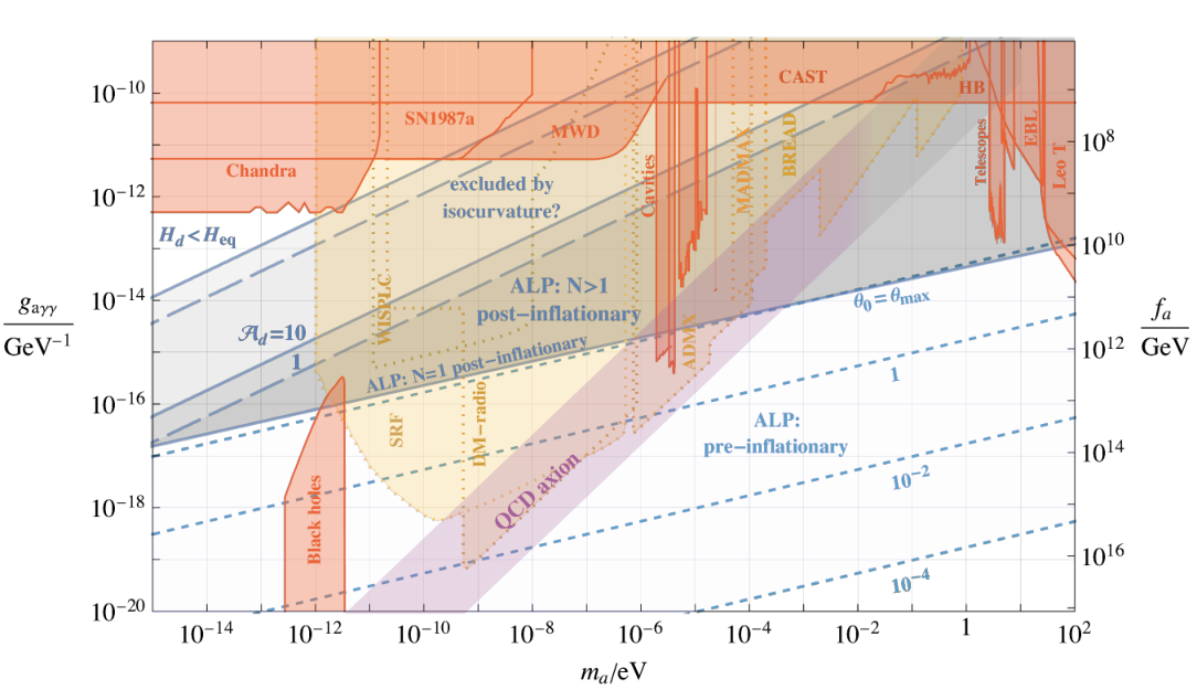
4.2 Relevance for experimental searches
The ALP-to-photon couplings in the pre- and post-inflationary scenarios are shown in Figure 4 imposing that . To enable comparison with existing and projected constraints we assume , so .1414 14 The current constraints on in Figure 4 come from various sources [77, 78, 79, 80, 81, 82, 83, 84, 85] (we do not attempt to be exhaustive and simply present the most important ones in each mass range). We also plot the bounds from black hole super-radiance, which do not require an axion-photon coupling [86, 87] and instead are relevant only for not too small, because a too large axion self-interaction hinders the super-radiance process. The axion-photon coupling for the QCD axion, given in eq. (2), is also shown; we set the upper and lower edges of the band by and respectively, but we stress that couplings outside the range plotted are possible (the band is grayed for because astrophysical observations rule out many such QCD axion theories [88, 89, 90, 91, 92]).
In Figure 4, dashed lines show the values of the initial misalignment angle for which an ALP in the pre-inflationary scenario makes up the full relic density. As can be seen, such an axion with can be all DM and compatible with existing constraints for almost any [93, 94, 95, 96, 82]. Meanwhile, an ALP in the post-inflationary scenario can make up the full dark matter abundance over the dark blue area as the value of the explicit symmetry breaking parameter , which determines , varies. Points with smaller (i.e. larger ) correspond to smaller , i.e. smaller . The upper edge of this region is set by the lowest allowed by isocurvature constraints, which depend on the uncertain parameters and (we also plot the weaker bound from requiring the domain wall network is destroyed before MRE). The lower edge of the post-inflationary region corresponds to so and the domain walls are destroyed soon after forming. In this case the DM abundance, and therefore , is of the same order as that in the post-inflationary scenario, which we calculate considering only the abundance produced by strings eq. (10) (if domain walls give a large contribution to the relic abundance the prediction would be at larger ).
4.3 Possible implications for gravitational wave searches
In a post-inflationary axion theory the evolution of the domain wall network between and produces a stochastic GW background [97, 61, 31, 32]. Due to the uncertainties in the dynamics of the network, the rate of production of these GWs is unknown. However, standard assumptions making use of the quadrupole approximation predict that the domain walls emit energy density in GWs at a rate roughly given by (see e.g. [98, 61, 31])
| (25) | ||||
If eq. (25) is accurate, the energy lost into GWs is much smaller than the total energy the network emits (in eq. (12)) over all of the allowed parameter space in Figure 4, and their backreaction is therefore not expected to affect the dynamics of the domain walls.
Because the domain walls have typical curvature of order Hubble, the instantaneous emission spectrum of the GWs is expected to be peaked at the Hubble parameter at the time of production. This is indeed the case in numerical simulations at small scale separations [61]. If true with the physical parameters, the GW spectrum today , where is the present-day GW frequency, will be peaked at the frequency corresponding to the Hubble parameter at the time the network is destroyed , i.e.
| (26) |
Assuming that eq. (25) reproduces the actual emission, the amplitude of the GW spectrum at its peak is
| (27) | ||||
Eq. (26) and the second line of eq. (27) follow from the expression for the axion relic abundance in eq. (15) and we allow for generality. As is evident from eq. (27), the strongest GW signals occur for the smallest allowed . This is because, for fixed and , smaller corresponds to smaller , so the GWs are redshifted less.
The possibility of observing these GWs is in tension with the observational bound on isocurvature perturbations described in Section 4.1: combing eq. (27) with eq. (23), the isocurvature bound implies
| (28) |
independent of and . For we have , and if the axion is only a small fraction of DM, this limit is not relaxed.1515 15 Meanwhile, the warm dark matter bound eq. (24), which applies if the axions are produced mildly relativistic, leads to . This is weaker than eq. (28) for (see also [32] for a related analysis). Near-future detectors are likely to only reach sensitivities for any frequency predicted by eq. (26).1616 16 Pulsar timing arrays will, at best, reach for frequencies around , and space based interferometers could have similar reach at higher frequencies. Because GWs redshift like radiation, the energy density they contain can be constrained by CMB observations [99], but current bounds are in the region of [100] and could be improved by only a few orders of magnitude (e.g. by the future EUCLID satellite). Finally, at frequencies measurements of the CMB polarisation data are relevant (see e.g. [101]). Current limits are for GWs of frequency [102, 103] (corresponding to ) and at higher frequencies these get weaker (planned experiments e.g. LiteBIRD [104], could have a factor better sensitivity). Therefore, unless the unknown constant (which parametrises the white-noise tail of the axion density power spectrum, see eq. (18)) is much smaller than the naive expectation, the allowed GW signals from ALP domain walls are barely detectable regardless of and . We do however stress that eq. (25) is just a rough parametric expectation, and an analysis of the GW emission from domain walls in numerical simulations taking into account the several required extrapolations would certainly be worthwhile, and left for future work. We also note that it is possible that the network stops emitting energy to axions efficiently enough to maintain an approximately constant at scale separations beyond the reach of simulations, completely altering the network’s dynamics and the resulting GW prediction.
GWs are also produced by the axion strings prior to [55] and the resulting stochastic background is detectable, compatibly with constraints from isocurvature perturbations, dark radiation, and axion dark matter overproduction, if , and . For such high however typical are suppressed and the relic axions cannot be directly detected (except for specific models e.g. based on [105, 106], where ).
4.4 Comments on ALP dark matter substructure
As discussed in Section 2.3, the decay of the string-domain wall network leads to order one fluctuations in the axion dark matter overdensity field at small spatial scales, which might lead to interesting dark matter substructure [107, 108, 109, 110, 63], see [111, 112, 113, 114, 115, 116, 117] for analysis in the case of the QCD axion. Although their properties are extremely uncertain, we now briefly comment on the evolution of an ALP’s initial fluctuations assuming that there are order-one overdensities on scales . As we will see, quantum pressure and axion self-interactions can play an important, previously neglected, role.
After the string-wall decays, the axion follows the nonrelativistic Schrödinger–Poisson EoM, which can be rewritten as the continuity and Euler equation of the density and velocity fields, and . At the small spatial scales we are interested in, . Nevertheless, we can obtain a qualitative understanding of the evolution of a generic mode (with comoving momentum ) by considering the linearised form of the EoM
| (29) |
where parametrises the axion quartic coupling , which we assume is attractive as is the case for a cosine potential (higher order couplings are present but negligible). The square bracket in eq. (29) is the Laplacian of the total potential acting on the field, where and are the ‘quantum’ pressure and self-interaction potentials respectively, while is the gravitational one, satisfying . Both and are attractive and tend to increase (given that ), while quantum pressure is repulsive and makes oscillate, preventing perturbations from collapsing. Note that eq. (29) reduces to the usual equation describing cold dark matter perturbations (the Meszaros equation) in the limits and . We refer to [118, 119, 120, 121, 122] for the derivation of eq. (29).
The EoM (29) takes a simplified form when expressed in terms of ,
| (30) |
where and and are two comoving momentum scales associated with quantum pressure (‘quantum’ Jeans scale [123]) and self-interactions, defined by
| (31) |
respectively, and the superscript ‘eq’ refers to quantities calculated at . For very IR modes ( and , which includes the normal adiabatic modes at cosmological scales) quantum pressure and self-interactions are negligible, and eq. (30) shows that such perturbations increase linearly around MRE as while order-one fluctuations collapse into bound objects at . However, for large enough quantum pressure and self-interactions affect the evolution by preventing the modes from collapsing, or enhancing their growth.
Interestingly, at MRE the quantum Jeans scale coincides with , modulo an order one factor:
| (32) |
similarly to vector bosons produced by inflationary fluctuations [124]. This relation holds regardless of the value of and even Newton’s constant (but it is modified if the axion mass is temperature dependent).1717 17 In eq. (32) we assume that the number of relativistic degrees of freedom at is given by the standard model high temperature value, which is appropriate for . However, the numerical factor in eq. (32) only depends on , so this has a negligible impact on our conclusions (e.g. of order 100 beyond Standard Model degrees of freedom around the TeV scale would not affect our conclusions).
In theories with the density power spectrum is expected to be peaked at with , where is a numerical factor that is highly uncertain (simulations at suggest [55] although this could be modified prior to MRE by free-streaming or, as we discuss shortly, self-interactions). Therefore, given eq. (32), the collapse of order-one fluctuations will be affected by quantum pressure unless , which would be surprising. In particular if quantum pressure will prevent fluctuations collapsing at MRE, and compact objects are not expected to form from these fluctuations.
Meanwhile, for all the values of and of interest , so at MRE the self-interactions do not affect the modes at or smaller. However, self-interactions could be important deep in radiation domination,1818 18 We thank Asimina Arvanitaki for pointing this out. when the corresponding terms in eqs. (29) and eq. (30) can be larger than the quantum pressure term because is proportional to the density. By solving eq. (30) starting at with , one can see that indeed perturbative modes at momenta grow substantially during radiation domination due to the self-interactions. This could significantly modify the initial spectrum of density fluctuations before the overdensities collapse. Given the large uncertainties on the initial spectrum, we leave a full study for future work.
Conversely, for the string network decays at a time when and the order one fluctuations are expected to lie on larger comoving scales, . The numerical value of , although unknown, might be , similarly to the scenario. At MRE, the ratio between the size of these fluctuations and the quantum Jeans scale reads
| (33) |
Thus, for (i.e. well within the blue region in the parameter space in Figure 4), quantum pressure is not expected to be relevant in the dynamics around MRE. Additionally, by solving eq. (30) starting at , self-interactions are also negligible throughout for modes or smaller. Thus, the order-one perturbations are expected to collapse into compact objects (miniclusters) with density , i.e. set by the average dark matter density when they collapse. The mass of the miniclusters will be similar to the mass contained within an initially order one fluctuation
| (34) | ||||
If , varies from roughly to over the allowed parameter space in Figure 4. Larger mass substructure will form at larger scales from the part of the initial density power spectrum, as these modes grow and collapse during matter domination, however the resulting clumps have lower density and are more likely to be subsequently destroyed by e.g. tidal disruption [124].
5 Discussion and future directions
We have shown that it is plausible that a post-inflationary axion-like-particle with can comprise the full dark matter abundance with values of that are fairly easily discoverable by several proposed haloscopes and are also relevant for searches using astrophysical observations, see Figure 4.1919 19 Among others, a post-inflationary ALP could be discovered by the experiments TOORAD [125], BREAD [126], BRASS [127], ORGAN [128], MADMAX [129], ALPHA [130], the next stages of ADMX, KLASH [131], DM-Radio [132], WISPLC [133], the broadband mode of ABRACADABRA [134], and searches with polaritons [135] (projections are not plotted for all of these). Meanwhile, parts of the parameter space are constrained by observations by the telescopes VIMOS [85] and MUSE [84] and extra-galactic background light (EBL), and the parameter space is close to bounds from measurements of the polarisation of photons emitted from magnetic white dwarf stars [80] (‘MWD’). Even larger are possible if the axion makes up only a fraction of the dark matter, but the discoverability in this case depends on the details of a particular experiment. Meanwhile, the DM substructure that is likely to form in theories with could provide complementary observational prospects. For instance, the miniclusters could be detected through gravitational interactions (e.g. by searches with pulsar timing arrays [136]) or via an ALP-photons coupling (e.g. by radio signals from collisions between miniclusters and neutron stars [137, 138, 139, 140]).2020 20 We note that the same theory can also lead to interesting signals if the string network survives until the time when the cosmic microwave background is formed and the axion makes up only a small fraction of DM [141].
Although large parts of our analysis have rested on analytic expectations, we have made some progress in studying the string-domain wall system with numerical simulations. In particular, we have provided evidence that increases proportionally to , see Figure 2. As a result, when extrapolated to the physical point (), is likely to take a value that is at least an order of magnitude larger than occurs in simulations. Such results are also directly applicable to the QCD axion, for which and , although the non-linear evolution of the axion waves at around in this case could affect the domain wall dynamics.
Of course many uncertainties remain. The evolution of the string-domain wall network and the area parameter at in theories is uncertain, and as a result the DM abundance is not known. Similarly, the density power spectrum of the relic axions is not reliably known. Although not a problem in our present work, the relation between the PQ symmetry breaking Lagrangian parameter and is also unknown apart from an analytic guess. This is particularly important for the QCD axion in the postinflationary scenario, because it determines whether the PQ breaking potential must be fine tuned, see e.g. [51, 97, 142, 60, 143].
The theory we focused on is quite minimal from a high energy perspective. All that is required is an axion potential with degenerate minima, a small breaking of the remaining discrete , and the PQ symmetry to be unbroken at the end of, or after, inflation. The first of these is typical for many sources of axion mass, e.g. if it comes from a strongly coupled hidden sector [144]. The second is not only easily accommodated but is thought to be inevitable [34, 35, 36]. Finally, for the we have considered, the PQ symmetry can easily be unbroken at the end of or after inflation: either due to quantum fluctuations during inflation, finite temperature effects after reheating, or a coupling between the inflaton and the radial mode [145, 146, 147, 148, 55, 149]. Additionally, it has recently been shown that, over most of the post-inflationary ALP parameter space in Figure 4, an ALP with a coupling to photons of the form eq. (3) with is only possible if the Standard Model gauge group does not arise from a grand unified theory with a QCD axion unless the Lagrangian is fine-tuned [150]. Consequently, as well as being relatively easily discoverable, a post-inflationary ALP could give remarkable information not only about the cosmological history of the Universe (because the PQ symmetry was unbroken after inflation) but also the high energy completion of the Standard Model.
Acknowledgements
We thank Asimina Arvanitaki for useful discussions and Giovanni Villadoro for discussions and collaboration on related work. EH thanks Jed Thompson, David Cyncynates, and Olivier Simon for useful discussions, and acknowledges the UK Science and Technology Facilities Council for support through the Quantum Sensors for the Hidden Sector collaboration under the grant ST/T006145/1 and UK Research and Innovation Future Leader Fellowship MR/V024566/1. We acknowledge use of the University of Liverpool Barkla HPC cluster and of the CINECA Marconi Skylake partition.
Appendix A More details on the pre-inflationary scenario
Here we summarise some standard results about ALP dark matter in the pre-inflationary scenario, focusing on the regime where the ALP is initially close to the top of a temperature independent cosine potential, i.e. (a similar analysis can be found in e.g. [118]). Such an initial condition does not correspond to a fine-tuning of a Lagrangian parameter. Rather, it is a ‘cosmological tuning’ in that our observable Universe corresponds to a rare part of the pre-inflationary, presumably random, axion field distribution.
For , numerical results for the function that enters the axion relic abundance in eq. (4) can be approximated by (to an accuracy of better than for )
| (35) |
where is fit numerically. Therefore, in this limit, to obtain full DM abundance requires
| (36) |
Therefore for a fixed the axion decay constant decreases only logarithmically with as
| (37) |
The smallest allowed in eq. (37) is determined by isocurvature bounds. Any scalar field that has mass smaller than during inflation obtains fluctuations during inflation that are of the order of . For the axion these are isocurvature and translate to fluctuations in the misalignment angle of
| (38) |
This induces isocurvature perturbations in the axion dark matter energy density at all scales of
| (39) | ||||
and an isocurvature contribution to (defined in eq. (17)) that is independent of . Observational constraints require [102], so, in the large misalignment limit,
| (40) |
which, in combination with eq. (36), leads to a lower bound on for a fixed if . For values are allowed. In principle somewhat smaller values of are compatible with cosmological observations provided reheating is fast enough that the Universe is radiation dominated before big bang nucleosynthesis. However, if our assumption that the axion starts oscillating at during radiation domination fails and the expression for the relic abundance will be modified in a way that depends on the particular cosmological history.
For completeness, we note that in the opposite regime , , so if the axion makes up all the dark matter the isocurvature constraint is . Thus, using eq. (4) with , the isocurvature bound is .
Appendix B The relic abundance from strings
Prior to the time when the string network should emit most of the axions at momentum , with a numerical factor that is expected to be based on simulation results. Consequently, the axion number density at a time as a result of emission prior to is
| (41) | ||||
where we used in the second line. Eq. (41) leads to an axion relic abundance given by eq. (10). On the other hand, between the times when and the majority of the energy is expected to be emitted into axions that are non-relativistic or at most mildly relativistic. As a result, at a time the axion number density from emission from strings after is
| (42) | ||||
Because , from eqs. (41) and (42) the majority of the axions are produced soon before and soon after the time when . Comparing with eq. (13), for , is much smaller than the number density emitted by domain walls, , during the same period. In particular, this is true once is small enough to overcome the logarithmic enhancement in eqs. (41) and (42).
Appendix C Simulations
C.1 Details of simulations
We solve the equations of motion of a complex scalar field with Lagrangian
| (43) |
in a Friedmann-Robertson-Walker background with scale factor , where is the cosmic time and the Hubble parameter . The potential is of the general form of eq. (6), and we choose the particular example
| (44) |
where . We follow [61] in multiplying the cosine in eq. (44) by factor of to avoid numerical instabilities (this has no effect away from the string cores). The magnitude of the final, breaking, term is parametrised by , related to defined in the main text by .2121 21 The choice that the minima of the preserving and breaking contributions to the potential coincide does not affect the dynamics. The EoM depend on only through the ratio , so we report different values of the axion mass always in terms of this. We solve the EoM on a discrete lattice of constant comoving size using a standard finite difference algorithm, typically on grids containing points.
The maximum ratios and that can be reached in simulations are limited by the combination of three requirements. First, the physical lattice spacing must be sufficiently small that the string and domain wall cores are resolved, i.e. and at all times. We pick , which we have checked is sufficient to not introduce the systematic uncertainties [53]. Second, while the network is present there must be at least a few Hubble patches within the simulation, i.e. where is the physical box size. We run simulations to (in Appendix C.3 we show this is safe from finite volume systematics). As a result, for the grid sizes that we use. Finally, must be sufficiently smaller than one so that the potential in eq. (44) leads to domain walls across which the radial mode stays close to its vacuum expectation value [151] , rather than interpolating across the top of its potential (such configurations are not the physical domain walls). In practice we find is sufficient, which in turn fixes .
We focus on the ‘fat string and domain wall’ system in which , and only consider the evolution of the physical theory (with constant) in simulations of the string scaling regime (i.e. prior to the time when ). In the fat string system, the number of lattice points inside string cores and domain walls remains constant in time. As mention in the main text, the fat string and domain wall system reaches the attractor faster. Moreover, modes with physical momentum or correspond to the same comoving momentum regardless of when they are produced, so energy emitted with momentum close to the string core scale () does not contaminate the spectrum at smaller momenta, during the scaling regime and the domain wall evolution.
Notice that the fat domain walls mean that the energy density emitted by the domain wall network per Hubble time evolves as rather than the physical , see eq. (12). However, because the energy density in axion waves redshifts , the relic abundance is still dominantly produced at late times. Additionally, the energy density in domain walls still dominates that in strings when .
We identify strings and domain walls using the algorithms in [151] and [152, 61] respectively and calculate the scaling parameters and from their definitions given in Section 2. As in the main text, when plotting results, it is convenient to measure the time in simulations in terms of or . Similarly to [53, 56] can be written in terms of the Fourier transforms and of the axion field and its time derivative respectively:
| (45) |
where is the magnitude of the axion comoving momentum , is the simulation volume, and is the solid angle.
C.2 The scaling parameters before network destruction
In this Appendix we show simulation results for the string length and the domain wall area parameter during the string scaling regime and after , as discussed in Section 2.2.
In Figure 5 (left) we plot the evolution of in the fat system for different values of the axion mass, normalised as (i.e. different ) with (meaning no breaking) and . This is analogous to the plot of in Figure 2 (left). For comparison, we also show the evolution in the absence of the axion mass, corresponding to the string scaling regime. For sufficiently small , has the well-known growth proportional to [151, 153, 53, 154]. deviates from the evolution at ; indicating that the domain walls that bound the strings at such times are affecting the dynamics. We do not attempt to extrapolate ’s evolution to large and . In Figure 5 (right) we plot the ratio as a function of for the fat and physical string systems with (black lines) and also with (coloured lines) for the fat strings, all with . For fat strings this ratio seems approximately constant while . Meanwhile, for the physical system with the evolution is less clear but is consistent with a slow approach to a constant ratio. The ratio in simulations with deviates from the evolution.
Finally, we give more details on the fit of prior to the time when , discussed in the main text. For the fat string system, the form in eq. (19) fits the data well, with consistent regardless of the in the range at which the fit is started. A quadratic ansatz of the kind results in compatible with zero but with a large uncertainty. The linear form in eq. (19) also fits the physical data well, but the best fit varies depending on the from which the fit is started. Considering the change in for initial between and , we estimate . We also note that in the physical case a quadratic fit of the previous form gives , slightly incompatible with zero.
C.3 Systematic uncertainties
Systematic uncertainties can arise in simulations in several ways: the finite lattice spacing, the finite volume, and the finite timestep. We have checked that our choices of simulation parameters are sufficient for all the observables that we extract from simulations to be unaffected. Since the analysis is very similar to that in [53], in this Appendix we simply demonstrate that our choice to end simulations when is sufficient for finite volume simulations to not affect (this is particularly important because the hint of a decrease in in Figure 2 right happens at the final times). To do so, in Figure 6 we plot and as a function of time for identical theories, but in boxes of different sizes, so that happens at different . After averaging over multiple runs, we see that there is no deviation in the mean and in the smaller simulations until well after they have . We have checked this remains the case regardless of , and .
References
- [1] R. D. Peccei and H. R. Quinn, “CP Conservation in the Presence of Instantons,” Phys. Rev. Lett. 38 (1977) 1440–1443.
- [2] S. Weinberg, “A New Light Boson?,” Phys. Rev. Lett. 40 (1978) 223–226.
- [3] F. Wilczek, “Problem of Strong and Invariance in the Presence of Instantons,” Phys. Rev. Lett. 40 (1978) 279–282.
- [4] J. E. Kim, “Weak Interaction Singlet and Strong CP Invariance,” Phys. Rev. Lett. 43 (1979) 103.
- [5] M. A. Shifman, A. I. Vainshtein, and V. I. Zakharov, “Can Confinement Ensure Natural CP Invariance of Strong Interactions?,” Nucl. Phys. B 166 (1980) 493–506.
- [6] A. R. Zhitnitsky, “On Possible Suppression of the Axion Hadron Interactions. (In Russian),” Sov. J. Nucl. Phys. 31 (1980) 260.
- [7] M. Dine, W. Fischler, and M. Srednicki, “A Simple Solution to the Strong CP Problem with a Harmless Axion,” Phys. Lett. B 104 (1981) 199–202.
- [8] P. Svrcek and E. Witten, “Axions In String Theory,” JHEP 06 (2006) 051, arXiv:hep-th/0605206.
- [9] A. Arvanitaki, S. Dimopoulos, S. Dubovsky, N. Kaloper, and J. March-Russell, “String Axiverse,” Phys. Rev. D 81 (2010) 123530, arXiv:0905.4720 [hep-th].
- [10] M. Cicoli, M. Goodsell, and A. Ringwald, “The type IIB string axiverse and its low-energy phenomenology,” JHEP 10 (2012) 146, arXiv:1206.0819 [hep-th].
- [11] B. S. Acharya, K. Bobkov, and P. Kumar, “An M Theory Solution to the Strong CP Problem and Constraints on the Axiverse,” JHEP 11 (2010) 105, arXiv:1004.5138 [hep-th].
- [12] M. Demirtas, N. Gendler, C. Long, L. McAllister, and J. Moritz, “PQ Axiverse,” arXiv:2112.04503 [hep-th].
- [13] J. Preskill, M. B. Wise, and F. Wilczek, “Cosmology of the Invisible Axion,” Phys. Lett. B 120 (1983) 127–132.
- [14] L. F. Abbott and P. Sikivie, “A Cosmological Bound on the Invisible Axion,” Phys. Lett. B 120 (1983) 133–136.
- [15] M. Dine and W. Fischler, “The Not So Harmless Axion,” Phys. Lett. B 120 (1983) 137–141.
- [16] P. Arias, D. Cadamuro, M. Goodsell, J. Jaeckel, J. Redondo, and A. Ringwald, “WISPy Cold Dark Matter,” JCAP 06 (2012) 013, arXiv:1201.5902 [hep-ph].
- [17] G. Alonso-Álvarez, R. S. Gupta, J. Jaeckel, and M. Spannowsky, “On the Wondrous Stability of ALP Dark Matter,” JCAP 03 (2020) 052, arXiv:1911.07885 [hep-ph].
- [18] P. Sikivie, “Experimental Tests of the Invisible Axion,” Phys. Rev. Lett. 51 (1983) 1415–1417. [Erratum: Phys.Rev.Lett. 52, 695 (1984)].
- [19] P. W. Graham, I. G. Irastorza, S. K. Lamoreaux, A. Lindner, and K. A. van Bibber, “Experimental Searches for the Axion and Axion-Like Particles,” Ann. Rev. Nucl. Part. Sci. 65 (2015) 485–514, arXiv:1602.00039 [hep-ex].
- [20] I. G. Irastorza and J. Redondo, “New experimental approaches in the search for axion-like particles,” Prog. Part. Nucl. Phys. 102 (2018) 89–159, arXiv:1801.08127 [hep-ph].
- [21] H. Georgi, D. B. Kaplan, and L. Randall, “Manifesting the Invisible Axion at Low-energies,” Phys. Lett. B 169 (1986) 73–78.
- [22] G. Grilli di Cortona, E. Hardy, J. Pardo Vega, and G. Villadoro, “The QCD axion, precisely,” JHEP 01 (2016) 034, arXiv:1511.02867 [hep-ph].
- [23] M. Gorghetto and G. Villadoro, “Topological Susceptibility and QCD Axion Mass: QED and NNLO corrections,” JHEP 03 (2019) 033, arXiv:1812.01008 [hep-ph].
- [24] M. Farina, D. Pappadopulo, F. Rompineve, and A. Tesi, “The photo-philic QCD axion,” JHEP 01 (2017) 095, arXiv:1611.09855 [hep-ph].
- [25] L. Darmé, L. Di Luzio, M. Giannotti, and E. Nardi, “Selective enhancement of the QCD axion couplings,” Phys. Rev. D 103 no. 1, (2021) 015034, arXiv:2010.15846 [hep-ph].
- [26] A. V. Sokolov and A. Ringwald, “Photophilic hadronic axion from heavy magnetic monopoles,” JHEP 06 (2021) 123, arXiv:2104.02574 [hep-ph].
- [27] M. Redi and A. Tesi, “The meso-inflationary QCD axion,” arXiv:2211.06421 [hep-ph].
- [28] K. Harigaya and L.-T. Wang, “More axions from diluted domain walls,” arXiv:2211.08289 [hep-ph].
- [29] D. Cyncynates, T. Giurgica-Tiron, O. Simon, and J. O. Thompson, “Resonant nonlinear pairs in the axiverse and their late-time direct and astrophysical signatures,” Phys. Rev. D 105 no. 5, (2022) 055005, arXiv:2109.09755 [hep-ph].
- [30] G. Alonso-Álvarez and J. Jaeckel, “Exploring axionlike particles beyond the canonical setup,” Phys. Rev. D 98 no. 2, (2018) 023539, arXiv:1712.07500 [hep-ph].
- [31] G. B. Gelmini, A. Simpson, and E. Vitagliano, “Gravitational waves from axionlike particle cosmic string-wall networks,” Phys. Rev. D 104 no. 6, (2021) 061301, arXiv:2103.07625 [hep-ph].
- [32] G. B. Gelmini, A. Simpson, and E. Vitagliano, “Catastrogenesis: DM, GWs, and PBHs from ALP string-wall networks,” arXiv:2207.07126 [hep-ph].
- [33] R. Zambujal Ferreira, A. Notari, O. Pujolàs, and F. Rompineve, “High Quality QCD Axion at Gravitational Wave Observatories,” arXiv:2107.07542 [hep-ph].
- [34] L. F. Abbott and M. B. Wise, “Wormholes and Global Symmetries,” Nucl. Phys. B 325 (1989) 687–704.
- [35] T. Banks and N. Seiberg, “Symmetries and Strings in Field Theory and Gravity,” Phys. Rev. D 83 (2011) 084019, arXiv:1011.5120 [hep-th].
- [36] D. Harlow and H. Ooguri, “Symmetries in quantum field theory and quantum gravity,” Commun. Math. Phys. 383 no. 3, (2021) 1669–1804, arXiv:1810.05338 [hep-th].
- [37] M. Kamionkowski and J. March-Russell, “Planck scale physics and the Peccei-Quinn mechanism,” Phys. Lett. B 282 (1992) 137–141, arXiv:hep-th/9202003.
- [38] S. M. Barr and D. Seckel, “Planck scale corrections to axion models,” Phys. Rev. D 46 (1992) 539–549.
- [39] S. Ghigna, M. Lusignoli, and M. Roncadelli, “Instability of the invisible axion,” Phys. Lett. B 283 (1992) 278–281.
- [40] B. Rai and G. Senjanovic, “Gravity and domain wall problem,” Phys. Rev. D 49 (1994) 2729–2733, arXiv:hep-ph/9301240.
- [41] R. Holman, S. D. H. Hsu, T. W. Kephart, E. W. Kolb, R. Watkins, and L. M. Widrow, “Solutions to the strong CP problem in a world with gravity,” Phys. Lett. B 282 (1992) 132–136, arXiv:hep-ph/9203206.
- [42] M. Dine, “Problems of naturalness: Some lessons from string theory,” in Conference on Topics in Quantum Gravity. 7, 1992. arXiv:hep-th/9207045.
- [43] B. A. Dobrescu, “The Strong CP problem versus Planck scale physics,” Phys. Rev. D 55 (1997) 5826–5833, arXiv:hep-ph/9609221.
- [44] P. Cox, T. Gherghetta, and M. D. Nguyen, “A Holographic Perspective on the Axion Quality Problem,” JHEP 01 (2020) 188, arXiv:1911.09385 [hep-ph].
- [45] S. Fichet and P. Saraswat, “Approximate Symmetries and Gravity,” JHEP 01 (2020) 088, arXiv:1909.02002 [hep-th].
- [46] W. Yin, “Scale and quality of Peccei-Quinn symmetry and weak gravity conjectures,” JHEP 10 (2020) 032, arXiv:2007.13320 [hep-ph].
- [47] A. Banerjee, J. Eby, and G. Perez, “From axion quality and naturalness problems to a high-quality QCD relaxion,” arXiv:2210.05690 [hep-ph].
- [48] T. W. B. Kibble, “Topology of Cosmic Domains and Strings,” J. Phys. A 9 (1976) 1387–1398.
- [49] A. Vilenkin, “Cosmic Strings,” Phys. Rev. D 24 (1981) 2082–2089.
- [50] A. Vilenkin and A. E. Everett, “Cosmic Strings and Domain Walls in Models with Goldstone and PseudoGoldstone Bosons,” Phys. Rev. Lett. 48 (1982) 1867–1870.
- [51] P. Sikivie, “Of Axions, Domain Walls and the Early Universe,” Phys. Rev. Lett. 48 (1982) 1156–1159.
- [52] P. Sikivie, “Axion Cosmology,” Lect. Notes Phys. 741 (2008) 19–50, arXiv:astro-ph/0610440.
- [53] M. Gorghetto, E. Hardy, and G. Villadoro, “Axions from Strings: the Attractive Solution,” JHEP 07 (2018) 151, arXiv:1806.04677 [hep-ph].
- [54] M. Buschmann, J. W. Foster, A. Hook, A. Peterson, D. E. Willcox, W. Zhang, and B. R. Safdi, “Dark matter from axion strings with adaptive mesh refinement,” Nature Commun. 13 no. 1, (2022) 1049, arXiv:2108.05368 [hep-ph].
- [55] M. Gorghetto, E. Hardy, and H. Nicolaescu, “Observing invisible axions with gravitational waves,” JCAP 06 (2021) 034, arXiv:2101.11007 [hep-ph].
- [56] M. Gorghetto, E. Hardy, and G. Villadoro, “More axions from strings,” SciPost Phys. 10 no. 2, (2021) 050, arXiv:2007.04990 [hep-ph].
- [57] Y. B. Zeldovich, I. Y. Kobzarev, and L. B. Okun, “Cosmological Consequences of the Spontaneous Breakdown of Discrete Symmetry,” Zh. Eksp. Teor. Fiz. 67 (1974) 3–11.
- [58] G. B. Gelmini, M. Gleiser, and E. W. Kolb, “Cosmology of Biased Discrete Symmetry Breaking,” Phys. Rev. D 39 (1989) 1558.
- [59] S. E. Larsson, S. Sarkar, and P. L. White, “Evading the cosmological domain wall problem,” Phys. Rev. D 55 (1997) 5129–5135, arXiv:hep-ph/9608319.
- [60] A. Ringwald and K. Saikawa, “Axion dark matter in the post-inflationary Peccei-Quinn symmetry breaking scenario,” Phys. Rev. D 93 no. 8, (2016) 085031, arXiv:1512.06436 [hep-ph]. [Addendum: Phys.Rev.D 94, 049908 (2016)].
- [61] T. Hiramatsu, M. Kawasaki, K. Saikawa, and T. Sekiguchi, “Axion cosmology with long-lived domain walls,” JCAP 01 (2013) 001, arXiv:1207.3166 [hep-ph].
- [62] A. Vaquero, J. Redondo, and J. Stadler, “Early seeds of axion miniclusters,” JCAP 04 (2019) 012, arXiv:1809.09241 [astro-ph.CO].
- [63] C. A. J. O’Hare, G. Pierobon, J. Redondo, and Y. Y. Y. Wong, “Simulations of axionlike particles in the postinflationary scenario,” Phys. Rev. D 105 no. 5, (2022) 055025, arXiv:2112.05117 [hep-ph].
- [64] E. W. Kolb and M. S. Turner, The Early Universe, vol. 69. 1990.
- [65] M. Feix, J. Frank, A. Pargner, R. Reischke, B. M. Schäfer, and T. Schwetz, “Isocurvature bounds on axion-like particle dark matter in the post-inflationary scenario,” JCAP 05 (2019) 021, arXiv:1903.06194 [astro-ph.CO].
- [66] V. Iršič, H. Xiao, and M. McQuinn, “Early structure formation constraints on the ultralight axion in the postinflation scenario,” Phys. Rev. D 101 no. 12, (2020) 123518, arXiv:1911.11150 [astro-ph.CO].
- [67] M. Feix, S. Hagstotz, A. Pargner, R. Reischke, B. M. Schäfer, and T. Schwetz, “Post-inflationary axion isocurvature perturbations facing CMB and large-scale structure,” JCAP 11 (2020) 046, arXiv:2004.02926 [astro-ph.CO].
- [68] P. Bode, J. P. Ostriker, and N. Turok, “Halo formation in warm dark matter models,” Astrophys. J. 556 (2001) 93–107, arXiv:astro-ph/0010389.
- [69] M. Viel, G. D. Becker, J. S. Bolton, and M. G. Haehnelt, “Warm dark matter as a solution to the small scale crisis: New constraints from high redshift Lyman- forest data,” Phys. Rev. D 88 (2013) 043502, arXiv:1306.2314 [astro-ph.CO].
- [70] V. Iršič et al., “New Constraints on the free-streaming of warm dark matter from intermediate and small scale Lyman- forest data,” Phys. Rev. D 96 no. 2, (2017) 023522, arXiv:1702.01764 [astro-ph.CO].
- [71] S. Baumholzer, V. Brdar, and E. Morgante, “Structure Formation Limits on Axion-Like Dark Matter,” JCAP 05 (2021) 004, arXiv:2012.09181 [hep-ph].
- [72] A. Dekker, S. Ando, C. A. Correa, and K. C. Y. Ng, “Warm Dark Matter Constraints Using Milky-Way Satellite Observations and Subhalo Evolution Modeling,” arXiv:2111.13137 [astro-ph.CO].
- [73] G. Ballesteros, M. A. G. Garcia, and M. Pierre, “How warm are non-thermal relics? Lyman- bounds on out-of-equilibrium dark matter,” JCAP 03 (2021) 101, arXiv:2011.13458 [hep-ph].
- [74] R. Diamanti, S. Ando, S. Gariazzo, O. Mena, and C. Weniger, “Cold dark matter plus not-so-clumpy dark relics,” JCAP 06 (2017) 008, arXiv:1701.03128 [astro-ph.CO].
- [75] M. A. Amin and M. Mirbabayi, “A lower bound on dark matter mass,” arXiv:2211.09775 [hep-ph].
- [76] C. O’Hare, “cajohare/axionlimits: Axionlimits.” https://cajohare.github.io/AxionLimits/, July, 2020.
- [77] J. S. Reynés, J. H. Matthews, C. S. Reynolds, H. R. Russell, R. N. Smith, and M. C. D. Marsh, “New constraints on light axion-like particles using Chandra transmission grating spectroscopy of the powerful cluster-hosted quasar H1821+643,” Mon. Not. Roy. Astron. Soc. 510 no. 1, (2021) 1264–1277, arXiv:2109.03261 [astro-ph.HE].
- [78] C. Dessert, J. W. Foster, and B. R. Safdi, “X-ray Searches for Axions from Super Star Clusters,” Phys. Rev. Lett. 125 no. 26, (2020) 261102, arXiv:2008.03305 [hep-ph].
- [79] M. Meyer and T. Petrushevska, “Search for Axionlike-Particle-Induced Prompt -Ray Emission from Extragalactic Core-Collapse Supernovae with the Large Area Telescope,” Phys. Rev. Lett. 124 no. 23, (2020) 231101, arXiv:2006.06722 [astro-ph.HE]. [Erratum: Phys.Rev.Lett. 125, 119901 (2020)].
- [80] C. Dessert, D. Dunsky, and B. R. Safdi, “Upper limit on the axion-photon coupling from magnetic white dwarf polarization,” arXiv:2203.04319 [hep-ph].
- [81] CAST Collaboration, V. Anastassopoulos et al., “New CAST Limit on the Axion-Photon Interaction,” Nature Phys. 13 (2017) 584–590, arXiv:1705.02290 [hep-ex].
- [82] D. Cadamuro and J. Redondo, “Cosmological bounds on pseudo Nambu-Goldstone bosons,” JCAP 02 (2012) 032, arXiv:1110.2895 [hep-ph].
- [83] D. Wadekar and Z. Wang, “Strong constraints on decay and annihilation of dark matter from heating of gas-rich dwarf galaxies,” arXiv:2111.08025 [hep-ph].
- [84] M. Regis, M. Taoso, D. Vaz, J. Brinchmann, S. L. Zoutendijk, N. F. Bouché, and M. Steinmetz, “Searching for light in the darkness: Bounds on ALP dark matter with the optical MUSE-faint survey,” Phys. Lett. B 814 (2021) 136075, arXiv:2009.01310 [astro-ph.CO].
- [85] D. Grin, G. Covone, J.-P. Kneib, M. Kamionkowski, A. Blain, and E. Jullo, “A Telescope Search for Decaying Relic Axions,” Phys. Rev. D 75 (2007) 105018, arXiv:astro-ph/0611502.
- [86] A. Arvanitaki, M. Baryakhtar, and X. Huang, “Discovering the QCD Axion with Black Holes and Gravitational Waves,” Phys. Rev. D 91 no. 8, (2015) 084011, arXiv:1411.2263 [hep-ph].
- [87] M. Baryakhtar, M. Galanis, R. Lasenby, and O. Simon, “Black hole superradiance of self-interacting scalar fields,” Phys. Rev. D 103 no. 9, (2021) 095019, arXiv:2011.11646 [hep-ph].
- [88] G. G. Raffelt, “Astrophysical axion bounds,” Lect. Notes Phys. 741 (2008) 51–71, arXiv:hep-ph/0611350.
- [89] J. H. Chang, R. Essig, and S. D. McDermott, “Supernova 1987A Constraints on Sub-GeV Dark Sectors, Millicharged Particles, the QCD Axion, and an Axion-like Particle,” JHEP 09 (2018) 051, arXiv:1803.00993 [hep-ph].
- [90] P. Carenza, T. Fischer, M. Giannotti, G. Guo, G. Martínez-Pinedo, and A. Mirizzi, “Improved axion emissivity from a supernova via nucleon-nucleon bremsstrahlung,” JCAP 10 no. 10, (2019) 016, arXiv:1906.11844 [hep-ph]. [Erratum: JCAP 05, E01 (2020)].
- [91] N. Viaux, M. Catelan, P. B. Stetson, G. Raffelt, J. Redondo, A. A. R. Valcarce, and A. Weiss, “Neutrino and axion bounds from the globular cluster M5 (NGC 5904),” Phys. Rev. Lett. 111 (2013) 231301, arXiv:1311.1669 [astro-ph.SR].
- [92] M. M. Miller Bertolami, B. E. Melendez, L. G. Althaus, and J. Isern, “Revisiting the axion bounds from the Galactic white dwarf luminosity function,” JCAP 10 (2014) 069, arXiv:1406.7712 [hep-ph].
- [93] V. Iršič, M. Viel, M. G. Haehnelt, J. S. Bolton, and G. D. Becker, “First constraints on fuzzy dark matter from Lyman- forest data and hydrodynamical simulations,” Phys. Rev. Lett. 119 no. 3, (2017) 031302, arXiv:1703.04683 [astro-ph.CO].
- [94] V. Lora, J. Magana, A. Bernal, F. J. Sanchez-Salcedo, and E. K. Grebel, “On the mass of ultra-light bosonic dark matter from galactic dynamics,” JCAP 02 (2012) 011, arXiv:1110.2684 [astro-ph.GA].
- [95] A. X. González-Morales, D. J. E. Marsh, J. Peñarrubia, and L. A. Ureña López, “Unbiased constraints on ultralight axion mass from dwarf spheroidal galaxies,” Mon. Not. Roy. Astron. Soc. 472 no. 2, (2017) 1346–1360, arXiv:1609.05856 [astro-ph.CO].
- [96] D. J. E. Marsh and J. C. Niemeyer, “Strong Constraints on Fuzzy Dark Matter from Ultrafaint Dwarf Galaxy Eridanus II,” Phys. Rev. Lett. 123 no. 5, (2019) 051103, arXiv:1810.08543 [astro-ph.CO].
- [97] S. Chang, C. Hagmann, and P. Sikivie, “Studies of the motion and decay of axion walls bounded by strings,” Phys. Rev. D 59 (1999) 023505, arXiv:hep-ph/9807374.
- [98] M. Maggiore, Gravitational Waves. Vol. 1: Theory and Experiments. Oxford Master Series in Physics. Oxford University Press, 2007.
- [99] T. L. Smith, E. Pierpaoli, and M. Kamionkowski, “A new cosmic microwave background constraint to primordial gravitational waves,” Phys. Rev. Lett. 97 (2006) 021301, arXiv:astro-ph/0603144.
- [100] L. Pagano, L. Salvati, and A. Melchiorri, “New constraints on primordial gravitational waves from Planck 2015,” Phys. Lett. B 760 (2016) 823–825, arXiv:1508.02393 [astro-ph.CO].
- [101] M. Kamionkowski and A. Kosowsky, “The Cosmic microwave background and particle physics,” Ann. Rev. Nucl. Part. Sci. 49 (1999) 77–123, arXiv:astro-ph/9904108.
- [102] Planck Collaboration, N. Aghanim et al., “Planck 2018 results. VI. Cosmological parameters,” Astron. Astrophys. 641 (2020) A6, arXiv:1807.06209 [astro-ph.CO]. [Erratum: Astron.Astrophys. 652, C4 (2021)].
- [103] BICEP2, Keck Array Collaboration, P. A. R. Ade et al., “BICEP2 / Keck Array x: Constraints on Primordial Gravitational Waves using Planck, WMAP, and New BICEP2/Keck Observations through the 2015 Season,” Phys. Rev. Lett. 121 (2018) 221301, arXiv:1810.05216 [astro-ph.CO].
- [104] T. Matsumura et al., “Mission design of LiteBIRD,” J. Low Temp. Phys. 176 (2014) 733, arXiv:1311.2847 [astro-ph.IM].
- [105] K. Choi and S. H. Im, “Realizing the relaxion from multiple axions and its UV completion with high scale supersymmetry,” JHEP 01 (2016) 149, arXiv:1511.00132 [hep-ph].
- [106] D. E. Kaplan and R. Rattazzi, “Large field excursions and approximate discrete symmetries from a clockwork axion,” Phys. Rev. D 93 no. 8, (2016) 085007, arXiv:1511.01827 [hep-ph].
- [107] C. J. Hogan and M. J. Rees, “AXION MINICLUSTERS,” Phys. Lett. B 205 (1988) 228–230.
- [108] E. W. Kolb and I. I. Tkachev, “Axion miniclusters and Bose stars,” Phys. Rev. Lett. 71 (1993) 3051–3054, arXiv:hep-ph/9303313.
- [109] K. M. Zurek, C. J. Hogan, and T. R. Quinn, “Astrophysical Effects of Scalar Dark Matter Miniclusters,” Phys. Rev. D 75 (2007) 043511, arXiv:astro-ph/0607341.
- [110] E. Hardy, “Miniclusters in the Axiverse,” JHEP 02 (2017) 046, arXiv:1609.00208 [hep-ph].
- [111] M. Fairbairn, D. J. E. Marsh, J. Quevillon, and S. Rozier, “Structure formation and microlensing with axion miniclusters,” Phys. Rev. D 97 no. 8, (2018) 083502, arXiv:1707.03310 [astro-ph.CO].
- [112] L. Visinelli and J. Redondo, “Axion Miniclusters in Modified Cosmological Histories,” Phys. Rev. D 101 no. 2, (2020) 023008, arXiv:1808.01879 [astro-ph.CO].
- [113] B. Eggemeier, J. Redondo, K. Dolag, J. C. Niemeyer, and A. Vaquero, “First Simulations of Axion Minicluster Halos,” Phys. Rev. Lett. 125 no. 4, (2020) 041301, arXiv:1911.09417 [astro-ph.CO].
- [114] D. Ellis, D. J. E. Marsh, and C. Behrens, “Axion Miniclusters Made Easy,” Phys. Rev. D 103 no. 8, (2021) 083525, arXiv:2006.08637 [astro-ph.CO].
- [115] D. Ellis, D. J. E. Marsh, B. Eggemeier, J. Niemeyer, J. Redondo, and K. Dolag, “Structure of Axion Miniclusters,” arXiv:2204.13187 [hep-ph].
- [116] V. Dandoy, T. Schwetz, and E. Todarello, “A self-consistent wave description of axion miniclusters and their survival in the galaxy,” arXiv:2206.04619 [astro-ph.CO].
- [117] X. Shen, H. Xiao, P. F. Hopkins, and K. M. Zurek, “Disruption of Dark Matter Minihaloes in the Milky Way environment: Implications for Axion Miniclusters and Early Matter Domination,” arXiv:2207.11276 [astro-ph.GA].
- [118] A. Arvanitaki, S. Dimopoulos, M. Galanis, L. Lehner, J. O. Thompson, and K. Van Tilburg, “Large-misalignment mechanism for the formation of compact axion structures: Signatures from the QCD axion to fuzzy dark matter,” Phys. Rev. D 101 no. 8, (2020) 083014, arXiv:1909.11665 [astro-ph.CO].
- [119] P.-H. Chavanis, “Collapse of a self-gravitating Bose-Einstein condensate with attractive self-interaction,” Phys. Rev. D 94 no. 8, (2016) 083007, arXiv:1604.05904 [astro-ph.CO].
- [120] P.-H. Chavanis, “Growth of perturbations in an expanding universe with Bose-Einstein condensate dark matter,” Astron. Astrophys. 537 (2012) A127, arXiv:1103.2698 [astro-ph.CO].
- [121] J.-c. Hwang and H. Noh, “Axion as a Cold Dark Matter candidate,” Phys. Lett. B 680 (2009) 1–3, arXiv:0902.4738 [astro-ph.CO].
- [122] A. Suárez and P.-H. Chavanis, “Hydrodynamic representation of the Klein-Gordon-Einstein equations in the weak field limit: General formalism and perturbations analysis,” Phys. Rev. D 92 (2015) 023510, arXiv:1503.07437 [gr-qc].
- [123] L. Hui, “Wave Dark Matter,” Ann. Rev. Astron. Astrophys. 59 (2021) 247–289, arXiv:2101.11735 [astro-ph.CO].
- [124] M. Gorghetto, E. Hardy, J. March-Russell, N. Song, and S. M. West, “Dark Photon Stars: Formation and Role as Dark Matter Substructure,” arXiv:2203.10100 [hep-ph].
- [125] D. J. E. Marsh, K.-C. Fong, E. W. Lentz, L. Smejkal, and M. N. Ali, “Proposal to Detect Dark Matter using Axionic Topological Antiferromagnets,” Phys. Rev. Lett. 123 no. 12, (2019) 121601, arXiv:1807.08810 [hep-ph].
- [126] BREAD Collaboration, J. Liu et al., “Broadband solenoidal haloscope for terahertz axion detection,” arXiv:2111.12103 [physics.ins-det].
- [127] “Brass website.” http://wwwiexp.desy.de/groups/astroparticle/brass/brassweb.htm.
- [128] B. T. McAllister, G. Flower, E. N. Ivanov, M. Goryachev, J. Bourhill, and M. E. Tobar, “The ORGAN Experiment: An axion haloscope above 15 GHz,” Phys. Dark Univ. 18 (2017) 67–72, arXiv:1706.00209 [physics.ins-det].
- [129] MADMAX Working Group Collaboration, A. Caldwell, G. Dvali, B. Majorovits, A. Millar, G. Raffelt, J. Redondo, O. Reimann, F. Simon, and F. Steffen, “Dielectric Haloscopes: A New Way to Detect Axion Dark Matter,” Phys. Rev. Lett. 118 no. 9, (2017) 091801, arXiv:1611.05865 [physics.ins-det].
- [130] M. Lawson, A. J. Millar, M. Pancaldi, E. Vitagliano, and F. Wilczek, “Tunable axion plasma haloscopes,” Phys. Rev. Lett. 123 no. 14, (2019) 141802, arXiv:1904.11872 [hep-ph].
- [131] D. Alesini, D. Babusci, D. Di Gioacchino, C. Gatti, G. Lamanna, and C. Ligi, “The KLASH Proposal,” arXiv:1707.06010 [physics.ins-det].
- [132] M. Silva-Feaver et al., “Design Overview of DM Radio Pathfinder Experiment,” IEEE Trans. Appl. Supercond. 27 no. 4, (2017) 1400204, arXiv:1610.09344 [astro-ph.IM].
- [133] Z. Zhang, O. Ghosh, and D. Horns, “WISPLC: Search for Dark Matter with LC Circuit,” arXiv:2111.04541 [hep-ex].
- [134] J. L. Ouellet et al., “First Results from ABRACADABRA-10 cm: A Search for Sub-eV Axion Dark Matter,” Phys. Rev. Lett. 122 no. 12, (2019) 121802, arXiv:1810.12257 [hep-ex].
- [135] A. Mitridate, T. Trickle, Z. Zhang, and K. M. Zurek, “Detectability of Axion Dark Matter with Phonon Polaritons and Magnons,” Phys. Rev. D 102 no. 9, (2020) 095005, arXiv:2005.10256 [hep-ph].
- [136] H. Ramani, T. Trickle, and K. M. Zurek, “Observability of Dark Matter Substructure with Pulsar Timing Correlations,” JCAP 12 (2020) 033, arXiv:2005.03030 [astro-ph.CO].
- [137] I. I. Tkachev, “Fast Radio Bursts and Axion Miniclusters,” JETP Lett. 101 no. 1, (2015) 1–6, arXiv:1411.3900 [astro-ph.HE].
- [138] M. S. Pshirkov, “May axion clusters be sources of fast radio bursts?,” Int. J. Mod. Phys. D 26 no. 07, (2017) 1750068, arXiv:1609.09658 [astro-ph.HE].
- [139] J. H. Buckley, P. S. B. Dev, F. Ferrer, and F. P. Huang, “Fast radio bursts from axion stars moving through pulsar magnetospheres,” Phys. Rev. D 103 no. 4, (2021) 043015, arXiv:2004.06486 [astro-ph.HE].
- [140] T. D. P. Edwards, B. J. Kavanagh, L. Visinelli, and C. Weniger, “Transient Radio Signatures from Neutron Star Encounters with QCD Axion Miniclusters,” Phys. Rev. Lett. 127 no. 13, (2021) 131103, arXiv:2011.05378 [hep-ph].
- [141] P. Agrawal, A. Hook, J. Huang, and G. Marques-Tavares, “Axion string signatures: a cosmological plasma collider,” JHEP 01 (2022) 103, arXiv:2010.15848 [hep-ph].
- [142] M. Kawasaki, K. Saikawa, and T. Sekiguchi, “Axion dark matter from topological defects,” Phys. Rev. D 91 no. 6, (2015) 065014, arXiv:1412.0789 [hep-ph].
- [143] K. A. Beyer and S. Sarkar, “Ruling out light axions: the writing is on the wall,” arXiv:2211.14635 [hep-ph].
- [144] H. Georgi, J. E. Kim, and H.-P. Nilles, “Hidden sector gaugino condensation and the model independent axion,” Phys. Lett. B 437 (1998) 325–330, arXiv:hep-ph/9805510.
- [145] L. A. Kofman and A. D. Linde, “Generation of Density Perturbations in the Inflationary Cosmology,” Nucl. Phys. B 282 (1987) 555.
- [146] E. T. Vishniac, K. A. Olive, and D. Seckel, “Cosmic Strings and Inflation,” Nucl. Phys. B 289 (1987) 717–734.
- [147] J. Yokoyama, “INFLATION CAN SAVE COSMIC STRINGS,” Phys. Rev. Lett. 63 (1989) 712.
- [148] H. M. Hodges and J. R. Primack, “Strings, texture and inflation,” Phys. Rev. D 43 (1991) 3155–3172.
- [149] Y. Bao, J. Fan, and L. Li, “Opening up window of post-inflationary QCD axion,” arXiv:2209.09908 [hep-ph].
- [150] P. Agrawal, M. Nee, and M. Reig, “Axion Couplings in Grand Unified Theories,” arXiv:2206.07053 [hep-ph].
- [151] L. Fleury and G. D. Moore, “Axion dark matter: strings and their cores,” JCAP 01 (2016) 004, arXiv:1509.00026 [hep-ph].
- [152] W. H. Press, B. S. Ryden, and D. N. Spergel, “Dynamical Evolution of Domain Walls in an Expanding Universe,” apj 347 (Dec., 1989) .
- [153] V. B. . Klaer and G. D. Moore, “The dark-matter axion mass,” JCAP 11 (2017) 049, arXiv:1708.07521 [hep-ph].
- [154] V. B. Klaer and G. D. Moore, “Global cosmic string networks as a function of tension,” JCAP 06 (2020) 021, arXiv:1912.08058 [hep-ph].