The Statistical Polarization Properties of Coherent Curvature Radiation by Bunches: Application to Fast Radio Burst RepeatersJournal: ApJ
Abstract
Fast radio bursts (FRBs) are extragalactic radio transients with millisecond duration and extremely high brightness temperature. Very recently, some highly circularly polarized bursts were found in a repeater, FRB 20201124A. The significant circular polarization might be produced by coherent curvature radiation by bunches with the line of sight (LOS) deviating from the bunch central trajectories. In this work, we carry out simulations to study the statistical properties of burst polarization within the framework of coherent curvature radiation by charged bunches in the neutron star magnetosphere for repeating FRBs. The flux is almost constant within the opening angle of the bunch. However, when the LOS derivates from the bunch opening angle, the larger the derivation, the larger the circular polarization but the lower the flux. We investigate the statistical distribution of circular polarization and flux of radio bursts from an FRB repeater, and find that most of the bursts with high circular polarization have a relatively low flux. Besides, we find that most of the depolarization degrees of bursts have a small variation in a wide frequency band. Furthermore, we simulate the polarization angle (PA) evolution and find that most bursts show a flat PA evolution within the burst phases, and some bursts present a swing of PA.
Keywords:
Radio bursts (1339); Radio transient sources (2008); Magnetars (992); Radiative processes (2055)I introduction
Fast radio bursts (FRBs) are millisecond duration radio transients (Lorimer et al. 2007; Keane et al. 2012; Thornton et al. 2013), and their physical origins are still mysterious. So far, there are hundreds of FRBs that have been detected, and a small fraction of them show repeating behaviors11 1 A Transient Name Server system for newly reported FRBs (Petroff & Yaron 2020, https://www.wis-tns.org,).. Recently, Bochenek et al. 2020 and CHIME/FRB Collaboration et al. 2020b reported that a bright FRB-like burst from a Galactic magnetar SGR J1935+2154, suggesting that magnetars are the very likely physical origins of FRBs. Many theoretical models have been proposed to explain FRBs (Platts et al. 2019; Zhang 2020; Xiao et al. 2021; Lyubarsky 2021, see details from ). According to the position of radiation region, they are classified into two categories: close-in models, i.e., inside the neutron star magnetosphere (Kumar et al. 2017; Yang & Zhang 2018; Yang & Zhang 2021; Lu et al. 2020; Wang et al. 2019; Wang et al. 2020, e.g.,) and far-away models, i.e., outside the neutron star magnetosphere (Lyubarsky 2014; Beloborodov 2020; Metzger et al. 2019; Margalit et al. 2020b, e.g.,).
Polarization is an important probe to study the emission mechanism and is related to the geometry of the emission region. The polarization features of FRBs appear diversity. Most FRBs have strong linear polarization (LP) fractions near 100 and have a flat PA across each pulse (Dai et al. 2021; Nimmo et al. 2021; CHIME/FRB Collaboration et al. 2019; Gajjar et al. 2018; Michilli et al. 2018). However, some sources (e.g., FRB 180301 and FRB 181112) show partial linear or circular polarization and PAs vary remarkably with time (Luo et al. 2020; Cho et al. 2020). Notably, an ‘S’ or ‘inverse S’ shape pattern generally can be observed in the radio pulsars (Lorimer & Kramer 2012). The profiles have been predicted by the rotating vector model (Radhakrishnan & Cooke 1969). A significant circular polarization (CP) was observed in an FRB repeater, FRB 20201124A (Jiang et al. 2022; Hilmarsson et al. 2021; Kumar et al. 2021; Xu et al. 2021). A burst with a significant CP fraction can be as high as 47 (Kumar et al. 2021). Surprisingly, the CP fraction can be up to 75 found in a good fraction of bursts (Xu et al. 2021). Very recently, Jiang et al. 2022 reported most of the bursts with low CP degree and a small part of bursts have CP fraction higher than . The highly CP fraction may be caused by an intrinsic radiation mechanism (Wang et al. 2022b; Wang et al. 2022c; Tong & Wang 2022) or propagation effects (Beniamini et al. 2022).
In this paper, we mainly investigate the statistical features of polarization of radio bursts from an FRB repeater within the framework of coherent curvature radiation for repeating FRBs, as proposed in some models (Kumar et al. 2017; Yang & Zhang 2018; Lu et al. 2020; Wang et al. 2019; Wang et al. 2020, e.g.,). The paper is organized as follows. We first discuss the coherent curvature emission by charged bunches in the neutron star magnetosphere in Section II. The statistical properties of polarization of radio bursts and the simulation results are shown in Section III. The results are discussed and summarized in Section IV. The convention in cgs units is used throughout this paper.
II FRBs from Coherent Curvature Emission by Charges in the Neutron Star Magnetosphere
Coherent curvature emission is emitted when the relativistic particles move along the curved magnetic field lines. Some models invoking coherent curvature emission by charged bunches can explain the radio emission of pulsars (Ruderman & Sutherland 1975; Sturrock et al. 1975; Elsaesser & Kirk 1976; Cheng & Ruderman 1977; Melikidze et al. 2000; Gil et al. 2004; Gangadhara et al. 2021) and FRBs (Katz 2014; Kumar et al. 2017; Yang & Zhang 2018; Ghisellini & Locatelli 2018; Lu & Kumar 2018; Katz 2018; Wang & Lai 2020; Wang et al. 2020; Cooper & Wijers 2021; Wang et al. 2022c). When the size of the charged bunch is smaller than the half wavelength, electromagnetic waves are coherently enhanced remarkably. If the mean space among bunches is much larger than , particles among bunches are incoherent (Yang & Zhang 2018; Wang et al. 2022c). The outflow from the neutron star polar cap is probably unsteady. Because of the interaction between near-surface parallel electric field and charged particles from the surface, the neutron star inner gap would generate inhomogeneous sparks (Ruderman & Sutherland 1975; Zhang & Qiao 1996; Gil & Sendyk 2000). These sparks of electron-positron pairs would form bunches in the magnetosphere of a neutron star by two-stream instability (Usov 1987; Asseo & Melikidze 1998; Melikidze et al. 2000). In this section, we mainly consider a three-dimensional bunch case to study the polarization properties of radio bursts from an FRB repeater.
Consider an electron that moves along a trajectory and the unit vector of the line of sight (LOS) is denoted by . We assume that a three-dimensional bunch is uniformly distributed in all directions of . A coherent summation of the amplitudes should replace the single amplitude for a three-dimensional bunch case. The total energy radiated per unit solid angle per unit frequency interval for the moving charges in the magnetosphere can be written as (Wang et al. 2022c)
| (1) |
where is the observed angular frequency, is the retarded time, is the speed of light, and is the elementary charge. are the maximum numbers for the identifiers of charge and the total number of positron is . is defined as the component of in the plane that is vertical to the LOS: , where , is the electron velocity. We define as the angle between the electron velocity direction and the -axis at = 0 for one trajectory, and is defined as the angle between the LOS and the trajectory plane. The total amplitude of th bunch projection at the plane perpendicular to the LOS is then given by (Wang et al. 2022c)
| (2) |
where is the opening angle of the bunch, is the angle of the footpoint for field line at the stellar surface, is the curvature radius, is the Lorentz factor of bunch, , and is the modified Bessel function, and are the lower and upper boundary of , and are the lower and upper boundary of , respectively. and are the polarized components of the amplitude along and , where is the unit vector pointing to the center of the instantaneous circle, and is defined. One can derive the Stokes parameters via the polarization amplitudes.
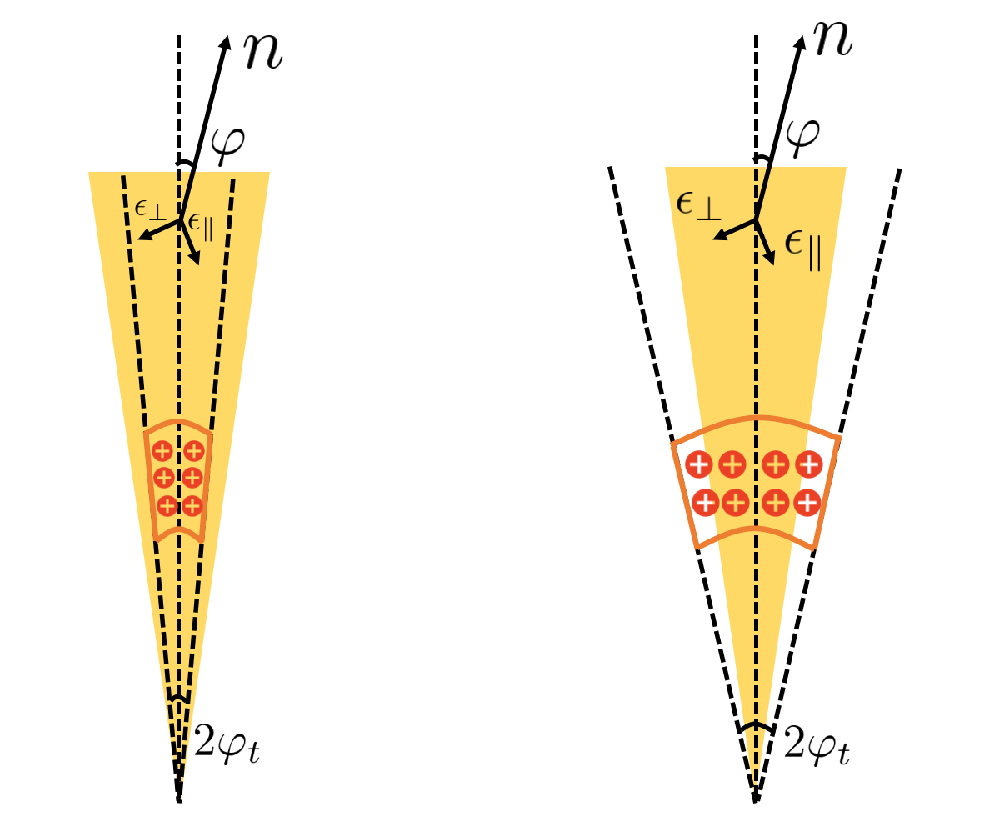
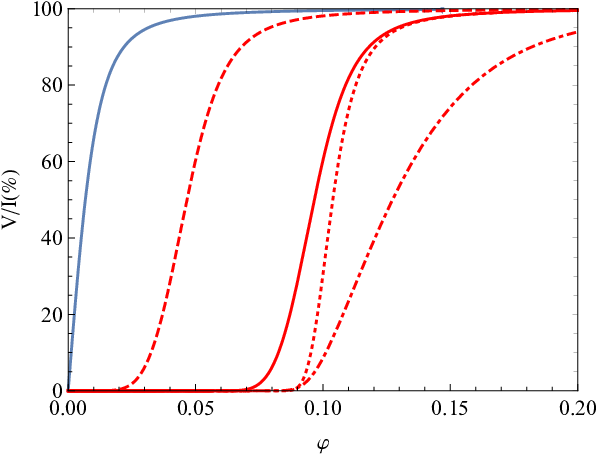
As shown in Figure 1, we consider the two cases for ( and ), and further study their polarization properties as follows. Figure 2 shows the CP as a function of the angle between the LOS and the trajectory plane (). The CP approaches slowly 100 as increases with a fixed , , and . A single charge case is different from the three-dimensional bunche case for . However, a single charge shares similar polarization properties with the bunch case of . Emitted radio waves have high LP if the LOS is limited to the beam within an angle of . In addition, the CP degree becomes stronger as grows, due to the non-axisymmetric summation of .
Within the framework of coherent curvature radiation by bunches, or bunch geometry can significantly affect the emission polarization. As shown in Figure 2, if becomes larger or becomes smaller, the red solid and dot-dashed lines will move in the direction of increasing . Therefore, we conclude that the less event rate for higher observed CP suggests that most highly linearly polarized bursts are generated within the emission cone. Besides, as becomes larger, we find the sharp evolution of CP with . The CP is difficult to be detected for the same LOS, since the decreases, leading to the original elliptical polarization is transformed into LP.
III The Statistical Properties of Polarization
III.1 The CP-Flux Properties
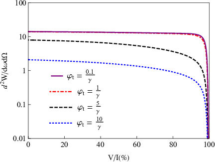
Within the framework of coherent curvature radiation by charged bunches, the CP is sensitive to the observed flux for the off-beam case. Some highly CP may appear at relatively low flux so that they generally are difficult to be detected by high sensitivity telescopes. In this section, we discuss the properties of CP-flux. According to Equations (1,2,), we can establish a relation between the flux and the CP. The flux as a function of CP for a three-dimensional bunch is shown in Figure 3. We find that the flux is roughly constant and the CP can be observed within the opening angle of bunches. The upper limit of CP can be limited for different . However, the deviation of the LOS from the direction of the velocity makes the highly circularly polarized emission hard to be observed since the flux drops rapidly. It is suggested that the flux is very sensitive for the off-beam case ().
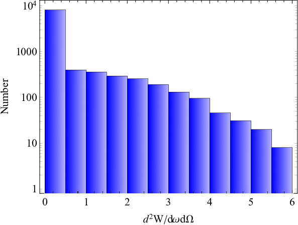

We consider the angle is randomly distributed in the range of to , the LOS range (from to ) should be larger than the range of bunch opening angle (from to ). The angle is a log-normal distribution in the range of to with a mean value of 22 2 In Figure 1, we consider the two cases for ( and ), should be included in this range., and the bunch length is a log-normal distribution in the range of 10 to 50 cm.33 3 The bunch length can be written as , which affects the enhancement factor due to coherence. (Yang & Zhang 2018; Wang et al. 2022c).. Assuming that the Lorentz factor, curvature radius, and angular frequency are constant (), we scatter 10000 points above the range of the parameters. We then get the and components, the CP, and flux can be calculated in the simulations.
As shown in the upper panel of Figure 4, we find that it has a more highly circularly polarized emission since more off-beam cases can appear. Besides, the smaller bunch opening angle trends appear in the off-beam case if the LOS is fixed. It can be seen from the simulation result (see the bottom panel of Figure 4) that the CP can be constrained with within an order of magnitude of the maximum flux of FRB (the red line). The maximum flux of an FRB in our simulation is defined by the condition of . The simulation of flux-CP shows that most of the bursts with high CP have relatively low flux. The burst energies spans for more than two orders of magnitude, and an artificial sharp cutoffs in the energy distributions due to the instrumental limitation (Jiang et al. 2022). We consider the flux threshold of FRBs times less than the maximum flux (the blue line). Therefore, bursts with highly CP are hardly observed since the flux is too low.
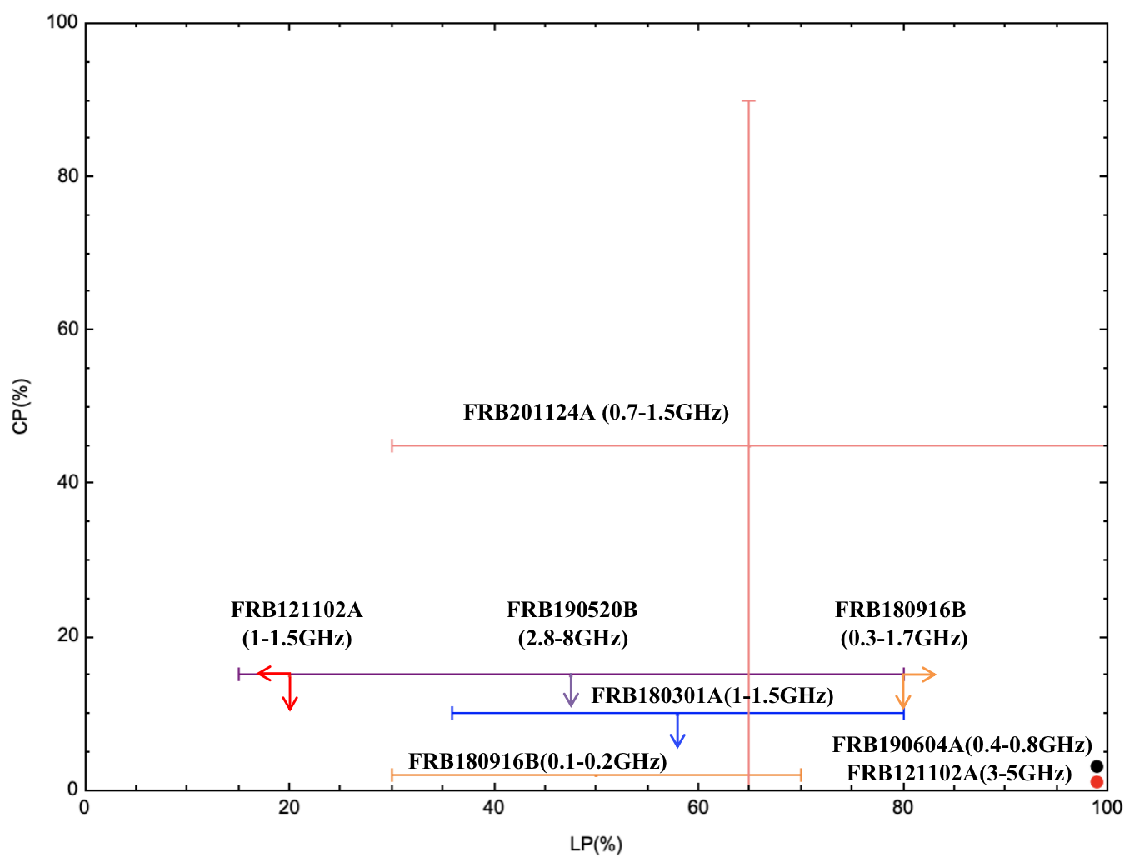
Some bursts with significant CP fraction can be as high as 75 (Xu et al. 2021), and a small fraction of the bursts have CP fraction higher than (Jiang et al. 2022). It is suggested that the bunch opening angle is smaller for a fixed LOS or the off-beam case. As shown in Figure 9, we plot the observed range of circular polarization (CP) fractions and linear polarization (LP) fractions for repeating FRBs (also see the statistical data from Table 1 by Wang et al. 2022a ). The CP fractions for most repeaters are . Besides, most of the bursts with low CP for FRB 20201124A (Jiang et al. 2022) indicate that most bunches have large opening angles to contribute to the low CP distribution (see the upper panel of Figure 5 ). Furthermore, the total degree of polarization is higher than 90 for most of the bursts of FRB 20201124A (Jiang et al. 2022). It is infered that the depolarization caused by the propagation effects basically can be neglected. Our simulation results are consistent with the representing observations.


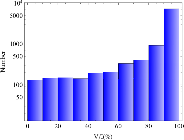
As shown in Figure 5, we also simulate the distribution of CP for different and . The upper panel of Figure 5 shows and varies from to . In our simulated results, we find of bursts have CP fraction higher than and of bursts have CP fraction smaller than for and varies from to , which is consistent with the observations of Jiang et al. 2022. Compared with Figure 4, the bunch opening angle is larger for the same LOS range or the upper limit of is smaller for the same (the bottom panel of Figure 5), making it has a more low CP distribution. It is consistent with the observations of Jiang et al. 2022. Since the larger bunch opening angle for the same LOS range, most low circularly polarized bursts are generated within the emission cone.
III.2 Depolarization for FRBs
Very recently, Feng et al. 2022 reported the polarization measurements of five active repeaters and found a trend of higher depolarization at lower frequencies. It can be well explained by the multipath propagation through a magnetized inhomogeneous plasma screen, and consistent with the observed temporal scattering (Yang et al. 2022). In this section, we consider the frequency-dependent LP fraction within the framework of coherent curvature radiation and simulate the distribution of depolarization degree.
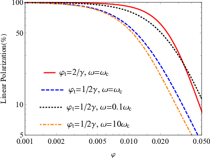
Polarized waves are generated by curvature radiation by relativistic particles streaming along curved magnetic field lines, which can be divided into the and components. The polarized waves is nearly 100 LP for . As shown in Figure 6, the LP decreases as the increases with a fixed and , which is attributed to the contribution. As the bunch opening angle becomes smaller (see the red and blue line of Figure 6), it is easier to appear the off-beam case, leading to the circularly polarized degree becomes strong. As shown in Figure 6 (see the blue, black, and orange lines), the depolarization degree has a small variation in a wide frequency band. We find the LP fraction decreases at higher frequencies within the framework of coherent curvature radiation. The result is very similar to the frequency dependence of pulsar LP (Morris et al. 1970; Manchester 1971). According to the radius-to-frequency mapping, high-frequency emission is generated from the lower magnetosphere, where the rotation effect gets weaker and the distribution regions of the two components (O-mode and X-mode) are overlapped (Wang et al. 2015). Thus, more significant depolarization would be observed for emission at a higher frequency. If the depolarization is caused by the propagation effect at the magnetosphere, a trend of lower LP at higher frequencies may be predicted.
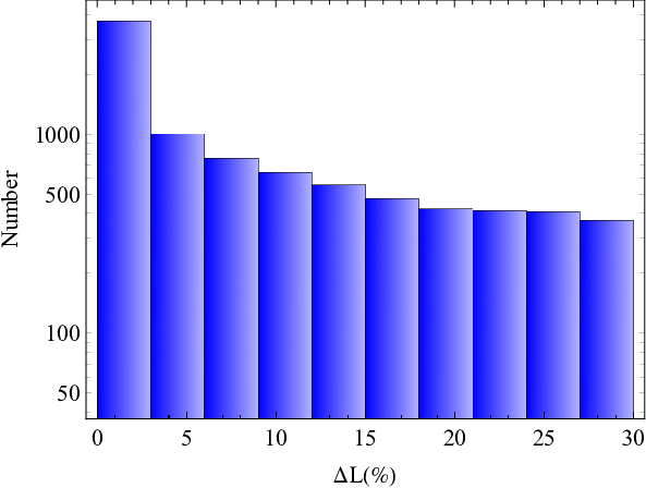
We simulate the distribution of depolarization degree within the framework of coherent curvature radiation and consider the angle is randomly distributed in the range of to , and the angle is a log-normal distribution in the range of to with a mean value of , and the frequency varies from 100 MHz to 10 GHz. The depolarization variation is shown in Figure 7, most of the depolarization degrees of bursts have a small variation in a wide frequency band. We also constrain the depolarization degree variation within 30 for the frequency varies from 100 MHz to 10 GHz. Feng et al. 2022 found the depolarization degree varies rapidly as the frequency for FRB sources. The larger depolarization infers that the rotation-measure scattering is large enough. The LP decreases by to low frequency for the FRBs with the frequency of half order of magnitude (Feng et al. 2022). However, Figure 7 shows that the depolarization varies within with the frequency of two orders of magnitude. Therefore, the contribution of the intrinsic curvature emission mechanism for the depolarization is very less than the rotation-measure scattering. It is consistent with the observation reported by Feng et al. 2022.
III.3 Simulated Polarization Angle Evolution
An ‘S’ or ‘inverse S’ shape pattern generally can be observed in the radio pulsars (Lorimer & Kramer 2012). The profiles have been predicted by the rotating vector model (Radhakrishnan & Cooke 1969). Some FRBs have a flat polarization angle across each pulse, which may be caused by the emission from the outer magnetosphere or a slowly rotating pulsar. However, emission from the inner magnetosphere or a quickly rotating pulsar could explain the rapid swing of polarization angle across each pulse for some FRBs. Besides, the spin and magnetic inclination of neutron star also affect the PA evolution. In this section, we mainly simulate the PA evolution. The polarization angle can be written as
| (4) |
where
| (5) |
and are the Stokes parameters. as a function of azimuthal angle with respect to the spin axis (Radhakrishnan & Cooke 1969).
| (6) |
where is the angle between the magnetic axis and the rotational axis, and is the angle between the LOS and spin axis.
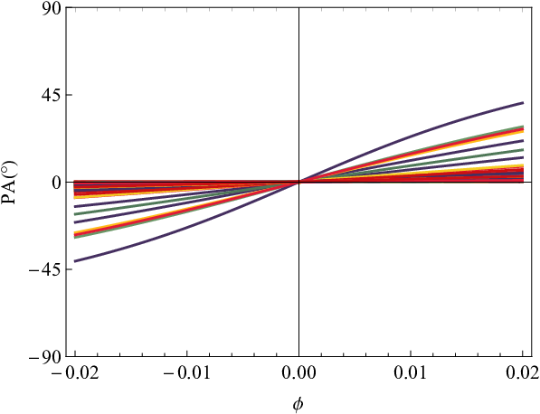

As shown in Figure 8, we simulate the PA evolution across each pulse and PA variation distribution. We consider the angle is randomly distributed in the range of to , and the angle is a log-normal distribution in the range of to ) with a mean value of for each pulse. Most bursts show a flat PA evolution within the burst phases, some bursts present a swing of PA across each pulse. A flat PA evolution for and the PA evolution is more dramatic for . We define the difference between maximum and minimum values of PA for each pulse as PA variation. We find the maximum change in the PA across the pulse profile is less than for most of the bursts, and a small fraction of bursts have the PA variation across each pulse higher than . It is suggested that most bursts have on-beam case to produce the small PA variation (e.g., FRB 20190520B, FRB 20121102A, FRB 20180301A, etc). Our simulated results are consistent with the predicted by Wang et al. 2022c and the observations (Jiang et al. 2022; Dai et al. 2021; Nimmo et al. 2021; CHIME/FRB Collaboration et al. 2019; Gajjar et al. 2018; Michilli et al. 2018; Luo et al. 2020; Cho et al. 2020). As shown in Figure 2, most of low CP bursts are generated within the emission cone. Therefore, the small PA variation is correlated with the low CP in the on-beam case. Our conclusions are consistent with the observations (see Figure 9).
IV Conclusions and Discussion
In this paper, we investigated the polarization features within the framework of coherent curvature radiation by charged bunches in the neutron star magnetosphere. We considered that FRBs are produced by coherent curvature radiation from bunches in the neutron star magnetosphere and discussed the statistical properties of polarization and the simulation results for radio bursts from an FRB repeater. The following conclusions can be drawn:
The CP across burst approaches slowly 100 as increases with a fixed ,, and . A single charge case is different from the three-dimensional bunche case for . However, the two cases are equivalent for , since the opening angle of the bunch can be seen as a point source case. Emitted radio waves have high LP if the LOS is limited to the beam within an angle of . While the CP degree becomes stronger as grows, due to the non-axisymmetric summation of . Within the framework of coherent curvature radiation, the bunch opening angle will significantly affect the polarization of emission. The less event rate for observed high CP suggests that most highly linearly polarized bursts are generated within the emission cone.
The flux is almost constant within the opening angle of bunches. However, when the LOS derivates from the bunch opening angle, the larger the derivation, the larger the CP but the lower the flux. We simulated the distribution of CP-flux, and found that most of the bursts with high CP have relatively low flux, and of bursts have CP fraction higher than and of bursts have CP fraction smaller than for and varies from to . Besides, the CP can be constrained with within an order of magnitude of the maximum flux of FRB for .
Most of the depolarization degrees of bursts have a small variation in a wide frequency band since the slow evolution of LP as frequency. We also constrained the depolarization variation within 30 for the frequency varies from 100 MHz to 10 GHz. Therefore, the contribution of the intrinsic curvature emission mechanism for the depolarization is very less than the rotation-measure scattering. Furthermore, we simulated the PA evolution and found that the maximum change in the PA across the pulse profile is less than for most of the bursts, and a small fraction of bursts have the PA variation across each pulse higher than . It is suggested that most bursts have on-beam case to produce the small PA variation. In conclusion, our simulation results are consistent with the representing observations (Jiang et al. 2022).
A significant CP was observed in an FRB repeater, FRB 20201124A (Jiang et al. 2022; Hilmarsson et al. 2021; Kumar et al. 2021; Xu et al. 2021). We considered that the high CP fraction may be caused by a coherent curvature radiation mechanism (Wang et al. 2022b; Wang et al. 2022c; Tong & Wang 2022). As shown in Figure 2, some important ingredients in the production of the CP are the geometric configuration of the bunch (e.g. the decreases for the same LOS), and the perpendicular flux increases. Although the CP fraction can be up to 75 for some bursts, depolarization exists in the process of incoherent summation of CP of opposite senses. It would cause some unpolarized emission. In addition, the CP is canceled by incoherent summation for the asymmetry of sparking distribution (Radhakrishnan & Rankin 1990; Wang et al. 2022c). Notably, Kumar et al. 2021 detected the CP of some bursts and the flux varies in a small range, the flux-CP shows a dispersion distribution. It is mainly caused by the fluctuation (e.g. the bunch length, opening angle).
According to the dipole magnetosphere geometry, the maximum cross section of the bunch can be approximately given by , where is the wavelength of the bunch, and is the radiation radius of the bunch. If there is a big phase gap between adjacent bunches, the emission is incoherent. The incoherent critical angle between adjacent magnetic lines is . Assuming = 10 cm and cm, we find . The fractional reduction in the LP amplitude can be given by , where is the intra-channel polarization position angle rotation. According to the above estimation, we can obtain the LP is nearly 100, and the depolarization degree is nearly 0. This result is consistent with the polarization observation of repeating FRBs (Dai et al. 2021; Nimmo et al. 2021; CHIME/FRB Collaboration et al. 2019; Gajjar et al. 2018; Michilli et al. 2018). Besides, Liu et al. 2020 simulated the LP distribution for the repeating FRBs and constrain the LP with for the FRBs with a flux of an order of magnitude lower than the maximum flux. However, the depolarization is mainly caused by the large differences of multi-path rotation measures when a radio wave propagates in the magneto-ionic inhomogeneous environment (Feng et al. 2022).
As shown in Section III.2, we have discussed the frequency-dependent linear polarization properties. We here discuss the time-dependent linear polarization properties, which would help test radiation mechanisms. The observed time-frequency is downward drifting from most repeating FRBs (Gajjar et al. 2018; Michilli et al. 2018; Hessels et al. 2019; Josephy et al. 2019; Caleb et al. 2020; Day et al. 2020; Platts et al. 2021). The time-frequency downward drifting is a natural consequence of coherent curvature radiation (Wang et al. 2019). A spark observed at an earlier time with a higher frequency is emitted in a more-curved magnetic field line. As shown in Figure 6, the LP fraction decreases at higher frequencies within the framework of coherent curvature radiation. Combined with the time-frequency observation properties of FRBs, we find that a lower linear polarization fraction is observed at an earlier time with a higher frequency for the same , and the depolarization degree has a small variation within the observation time. The above time-dependent linear polarization properties can be used to test the radiation mechanism of FRBs.
PA evolution generally involves two effects: the rotation radiation beam based on the rotating vector model (Radhakrishnan & Cooke 1969) and off-axis polarization properties of curvature radiation. According to the rotation vector model, the PA is flat for a slow rotating pulsar but evolves at near the smallest impact angle. The Stokes parameters and of this accumulated emission also play a part in PA evolution. A flat PA evolution (e.g. FRB 121102, FRB 180916, and FRB 20201124A) indicates a slow rotating pulsar and on-beam case. Variable PA evolution (FRB 180301, 181112) may need more complicated magnetic field configurations and LOS geometry.
Motivated by an inverse Compton scattering (ICS) model of radio pulsar radiation (Qiao & Lin 1998; Xu et al. 2000). Recently, Zhang 2022 proposed a model invoking coherent ICS by bunches as the radiation mechanism of FRBs. Considering the coherency of the radiation from a bunch of electrons, the radio radiation of pulsar from the lower emission altitudes would produce the CP (Xu et al. 2000). The polarization properties of the scattered photons will be affected by the asymmetrical particle distribution, the angular frequency of the scattered wave, and so on. We will further study the spectra and polarization features of the coherent ICS model in our future work.
References
- Anna-Thomas et al. (2022) Anna-Thomas R., Connor L., Burke-Spolaor S., Beniamini P., Aggarwal K., Law C. J., Lynch R. S., et al., 2022, arXiv, arXiv:2202.11112
- Asseo & Melikidze (1998) Asseo, E. & Melikidze, G. I. 1998, MNRAS, 301, 59
- Beloborodov (2020) Beloborodov, A. M. 2020, ApJ, 896, 142
- Beniamini et al. (2022) Beniamini, P., Kumar, P., & Narayan, R. 2022, MNRAS, 510, 4654
- Bochenek et al. (2020) Bochenek, C. D., Ravi, V., Belov, K. V., et al. 2020, Nature, 587, 59
- Caleb et al. (2020) Caleb, M., Stappers, B. W., Abbott, T. D., et al. 2020, MNRAS, 496, 4565
- Cheng & Ruderman (1977) Cheng, A. F. & Ruderman, M. A. 1977, ApJ, 212, 800
- CHIME/FRB Collaboration et al. (2020b) CHIME/FRB Collaboration, Andersen, B. C., Bandura, K. M., Bhardwaj, M., et al. 2020b, Nature, 587, 54
- CHIME/FRB Collaboration et al. (2019) CHIME/FRB Collaboration, Andersen, B. C., Bandura, K., et al. 2019, ApJ, 885, L24
- Cho et al. (2020) Cho, H., Macquart, J.-P., Shannon, R. M., et al. 2020, ApJ, 891, L38
- Cooper & Wijers (2021) Cooper, A. J. & Wijers, R. A. M. J. 2021, MNRAS, 508, L32
- Dai et al. (2022) Dai S., Feng Y., Yang Y. P., Zhang Y. K., Li D., Niu C. H., Wang P., et al., 2022, arXiv, arXiv:2203.08151
- Dai et al. (2021) Dai, S., Lu, J., Wang, C., et al. 2021, ApJ, 920, 46
- Day et al. (2020) Day, C. K., Deller, A. T., Shannon, R. M., et al. 2020, MNRAS, 497, 3335
- Elsaesser & Kirk (1976) Elsaesser, K. & Kirk, J. 1976, A&A, 52, 449
- Feng et al. (2022) Feng, Y., Li, D., Yang, Y.-P., et al. 2022, Science, 375, 1266
- Fonseca et al. (2020) Fonseca, E., Andersen, B. C., Bhardwaj, M., et al. 2020, ApJ, 891, L6
- Gajjar et al. (2018) Gajjar, V., Siemion, A. P. V., Price, D. C., et al. 2018, ApJ, 863, 2
- Gangadhara et al. (2021) Gangadhara, R. T., Han, J. L., & Wang, P. F. 2021, ApJ, 911, 152
- Ghisellini & Locatelli (2018) Ghisellini, G., & Locatelli, N. 2018, A&A, 613, A61
- Gil et al. (2004) Gil, J., Lyubarsky, Y., & Melikidze, G. I. 2004, ApJ, 600, 872
- Gil & Sendyk (2000) Gil, J. A. & Sendyk, M. 2000, ApJ, 541, 351
- Hessels et al. (2019) Hessels, J. W. T., Spitler, L. G., Seymour, A. D., et al. 2019, ApJ, 876, L23
- Hilmarsson et al. (2021) Hilmarsson, G. H., Michilli, D., Spitler, L. G., et al. 2021, ApJ, 908, L10
- Hilmarsson et al. (2021) Hilmarsson, G. H., Spitler, L. G., Main, R. A., et al. 2021, MNRAS, 508, 5354
- Jiang et al. (2022) Jiang, J.-C., Wang, W.-Y., Xu, H., et al. 2022, arXiv:2210.03609
- Josephy et al. (2019) Josephy, A., Chawla, P., Fonseca, E., et al. 2019, ApJ, 882, L18
- Katz (2014) Katz, J. I. 2014, Phys. Rev. D, 89, 103009
- Katz (2018) Katz, J. I. 2018, MNRAS, 481, 2946
- Keane et al. (2012) Keane, E. F., Stappers, B. W., Kramer, M., & Lyne, A. G. 2012, MNRAS, 425, L71
- Kumar et al. (2017) Kumar, P., Lu, W., & Bhattacharya, M. 2017, MNRAS, 468, 2726
- Kumar et al. (2021) Kumar, P., Shannon, R. M., Lower, M. E., et al. 2021, arXiv:2109.11535
- Liu et al. (2020) Liu, Z.-N., Wang, W.-Y., Yang, Y.-P., & Dai, Z. G. 2020, ApJ, 905, 140
- Lorimer et al. (2007) Lorimer, D. R., Bailes, M., McLaughlin, M. A., Narkevic, D. J.,& Crawford, F. 2007, Science, 318, 777
- Lorimer & Kramer (2012) Lorimer, D. R. & Kramer, M. 2012, Handbook of Pulsar Astronomy, by D. R. Lorimer, M. Kramer, Cambridge, UK: Cambridge University Press, 2012
- Lu & Kumar (2018) Lu, W. & Kumar, P. 2018, MNRAS, 477, 2470
- Lu et al. (2020) Lu, W., Kumar, P., & Zhang, B. 2020, MNRAS, 498, 1397
- Luo et al. (2020) Luo, R., Wang, B. J., Men, Y. P., et al. 2020, Nature, 586, 693
- Lyubarsky (2014) Lyubarsky, Y. 2014, MNRAS, 442, L9
- Lyubarsky (2021) Lyubarsky, Y. 2021, Universe, 7, 56
- Manchester (1971) Manchester, R. N. 1971, ApJS, 23, 283
- Margalit et al. (2020b) Margalit, B., Metzger, B. D., & Sironi, L. 2020, MNRAS, 494, 4627
- Melikidze et al. (2000) Melikidze, G. I., Gil, J. A., & Pataraya, A. D. 2000, ApJ, 544, 1081
- Metzger et al. (2019) Metzger, B. D., Margalit, B., & Sironi, L. 2019, MNRAS, 485, 4091
- Michilli et al. (2018) Michilli, D., Seymour, A., Hessels, J. W. T., et al. 2018, Nature, 553, 182
- Morris et al. (1970) Morris, D., Schwarz, U. J., & Cooke, D. J. 1970, Astrophys. Lett., 5, 181
- Nimmo et al. (2021) Nimmo, K., Hessels, J. W. T., Keimpema, A., et al. 2021, Nature Astronomy, 5, 594
- Niu et al. (2022) Niu, C.-H., Aggarwal, K., Li, D., et al. 2022, Nature, 606, 873
- Petroff & Yaron (2020) Petroff, E. & Yaron, O. 2020, Transient Name Server AstroNote, 160
- Platts et al. (2021) Platts, E., Caleb, M., Stappers, B. W., et al. 2021, MNRAS, 505, 3041
- Platts et al. (2019) Platts, E., Weltman, A., Walters, A., et al. 2019, Phys. Rep., 821, 1
- Plavin et al. (2022) Plavin, A., Paragi, Z., Marcote, B., et al. 2022, MNRAS, 511, 6033
- Pleunis et al. (2021) Pleunis, Z., Michilli, D., Bassa, C. G., et al. 2021, ApJ, 911, L3
- Qiao & Lin (1998) Qiao, G. J. & Lin, W. P. 1998, A&A, 333, 172
- Radhakrishnan & Cooke (1969) Radhakrishnan, V. & Cooke, D. J. 1969, Astrophys. Lett., 3, 225
- Radhakrishnan & Rankin (1990) Radhakrishnan, V. & Rankin, J. M. 1990, ApJ, 352, 258
- Ruderman & Sutherland (1975) Ruderman, M. A. & Sutherland, P. G. 1975, ApJ, 196, 51
- Sand et al. (2022) Sand, K. R., Faber, J. T., Gajjar, V., et al. 2022, ApJ, 932, 98
- Sturrock et al. (1975) Sturrock, P. A., Petrosian, V., & Turk, J. S. 1975, ApJ, 196, 73
- Thornton et al. (2013) Thornton, D., Stappers, B., Bailes, M., et al. 2013, Science, 341, 53
- Tong & Wang (2022) Tong, H. & Wang, H. G. 2022, arXiv:2202.05475
- Usov (1987) Usov, V. V. 1987, ApJ, 320, 333
- Wang & Lai (2020) Wang, J.-S. & Lai, D. 2020, ApJ, 892, 135
- Wang et al. (2015) Wang, P. F., Wang, C., & Han, J. L. 2015, MNRAS, 448, 771
- Wang et al. (2022a) Wang, W.-Y., Jiang, J.-C., Lee, K., et al. 2022a, MNRAS, 517, 5080
- Wang et al. (2022b) Wang, W.-Y., Jiang, J.-C., Lu, J., et al. 2022b, Science China Physics, Mechanics, and Astronomy, 65, 289511
- Wang et al. (2020) Wang, W.-Y., Xu, R., & Chen, X. 2020, ApJ, 899, 109
- Wang et al. (2022c) Wang, W.-Y., Yang, Y.-P., Niu, C.-H., et al. 2022c, ApJ, 927, 105
- Wang et al. (2019) Wang, W.-Y., Zhang, B., Chen, X., et al. 2019, ApJ, 876, L15
- Xiao et al. (2021) Xiao, D., Wang, F. Y., & Dai, Z.-G. 2021, Science China Physics, Mechanics, and Astronomy, 64, 249501
- Xu et al. (2000) Xu, R. X., Liu, J. F., Han, J. L., et al. 2000, ApJ, 535, 354
- Xu et al. (2021) Xu, H., Niu, J. R., Chen, P., et al. 2021, arXiv:2111.11764
- Yang et al. (2022) Yang, Y.-P., Lu, W., Feng, Y., et al. 2022, ApJ, 928, L16
- Yang & Zhang (2018) Yang, Y.-P., & Zhang, B. 2018, ApJ, 868, 31
- Yang & Zhang (2021) Yang, Y.-P. & Zhang, B. 2021, ApJ, 919, 89
- Zhang (2020) Zhang, B. 2020, Nature, 587, 45
- Zhang (2022) Zhang, B. 2022, ApJ, 925, 53
- Zhang & Qiao (1996) Zhang, B. & Qiao, G. J. 1996, A&A, 310, 135