Quantum enhanced probing of multilayered-samples
Abstract
Quantum sensing exploits quantum phenomena to enhance the detection and estimation of classical parameters of physical systems and biological entities, particularly so as to overcome the inefficiencies of its classical counterparts. A particularly promising approach within quantum sensing is Quantum Optical Coherence Tomography which relies on non-classical light sources to reconstruct the internal structure of multilayered materials. Compared to traditional classical probing, Quantum Optical Coherence Tomography provides enhanced-resolution images and is unaffected by even-order dispersion. One of the main limitations of this technique lies in the appearance of artifacts and echoes, i.e. fake structures that appear in the coincidence interferogram, which hinder the retrieval of information required for tomography scans. Here, by utilizing a full theoretical model, in combination with a fast genetic algorithm to post-process the data, we successfully extract the morphology of complex multilayered samples and thoroughly distinguish real interfaces, artifacts, and echoes. We test the effectiveness of the model and algorithm by comparing its predictions to experimentally-generated interferograms through the controlled variation of the pump wavelength. Our results could potentially lead to the development of practical high-resolution probing of complex structures and non-invasive scanning of photo-degradable materials for biomedical imaging/sensing, clinical applications, and materials science.
I Introduction
Quantum sensing is one of the emerging technologies that exploits quantum correlations and entanglement for detecting and imaging classical objects with fundamentally better performance while providing opportunities to overcome the limitations and challenges of the traditional classical approaches RMP; Rev2; PhysRevLett.114.080503; Pirandola2018; radar; rev3; Giovannetti2011; PhysRevA.107.032611; Salari2023. One of the well-developed and powerful methods of quantum sensing is Quantum Optical Coherence Tomography (QOCT) that utilizes the unique features of entangled photon pairs to image different layers within a sample of interest Abouraddy_2002; NASR20091154; Teich2012; Lopez-Mago:12; Lavoie:09; Yepiz_2019; ebi. This quantum imaging technique offers unprecedented capabilities in biomedical imaging nasr_2009; yepiz-borja_2022 and full-field scanning of samples using cameras with a single-photon sensitivity Ibarra-Borja_2020; Bienvenu_ndagano_2022. Compared to its classical counterpart, QOCT offers higher image (axial) resolution by a factor of 2 and provides immunity to even-order dispersion effects, the latter ensured by strict frequency anti-correlation.
Nonetheless, the vast practicality of QOCT is often hampered by long acquisition times and the problem of artifacts, i.e. fake structures appearing as peaks or dips in the coincidence interferograms that corrupt the QOCT signal and hinder the proper interpretation of tomography scans. Such fake structures are inherent to the system due to the quantum nature of QOCT. Note also that this difficulty becomes increasingly acute as the sample complexity, in terms of the number of interfaces, increases. For even a modest number of interfaces, peak/dip discrimination can become an extremely challenging task. Previous works have developed tools geared at correctly inferring the sample morphology from the QOCT interferogram through artifact removal. In Ref. Yepiz_2019 a specific method was demonstrated for suppressing cross-interference artifacts based on Spontaneous Parametric Down Conversion (SPDC) photon pairs produced by a broadband, femtosecond-duration pump. At the core of this technique is the existence of multiple pump wavelengths, which leads to the possibility of spectrally sweeping a continuous-wave pump and averaging the resulting interferograms as an alternative method. It has been shown that artifact removal can likewise be attained through the Fourier transformation properties of the two-dimensional joint spectrum Kolenderska:20; Kolenderska_2021, and using deep-learning techniques Liu_22. Both artifact removal approaches are based on a theoretical framework that is limited to a model based on only two interfaces and which requires processes that are prone to loss of relevant information. Moreover, such models have disregarded the presence of additional structures appearing in the QOCT interferogram which, though neglected, have a large impact on the signal as a whole.
In this work, rather than focusing directly on artifact removal, we aim first to develop a QOCT model which fully takes into account all observed effects, some of which have been neglected in past work. This includes multiple reflections in the sample, leading to echoes which behave as virtual interfaces, as well as cross-interference artifacts between a real interface and an echo, and even cross-interference artifacts between two echoes. As will become clear below, on the one hand these effects can be significant for realistic situations, and on the other hand, multiple terms can contribute to a given interferogram peak/dip so that attempting to infer the sample morphology without an adequate physical understanding will yield misleading results. Armed with a full understanding of the relevant optical effects that occur in the sample, in this work we aim secondly at developing a computational tool, based on genetic algorithms, that can predict the morphology which best fits a particular observed QOCT interferogram. Through this approach, we are particularly able to extract sample parameters (layer optical thicknesses and interface reflectivities) from the QOCT interferogram. Our methodology will help to accurately interpret the often highly-complex interferograms which result from realistic samples and consequently pave the way toward the practical implementation of quantum scanning and probing.
II Theoretical modeling
II.1 Multi-layer sample description and QOCT signal
As shown in Fig. 1, QOCT is generally based on Hong-Ou-Mandel (HOM) ebi interferometry in which pairs of entangled photons, typically generated through SPDC, are split and conducted through two different paths. The signal photon travels through a reference path of known length, while the idler photon passes through a sample arm which reflects light back from each of the multiple interfaces in a sample. The signal and idler photons are then recombined at a beamsplitter where HOM interference occurs and, provided that the two photons are indistinguishable, will exit the same port in a process referred to as bunching. Photon-bunching is more likely to happen when the temporal delay between the signal and idler photons is zero (); that is, when the path lengths of the reference arm and the sample arm are equal. The HOM interference is characterized by a drop in the coincidence count rate, or HOM dip, of the output joint detection at . Thus, for every interface, a corresponding HOM dip will appear in the coincidence rate signal , resulting in a sequence of dips in the interferogram obtained from a multilayer sample.
In order to describe the QOCT output signal, we consider a non-conservative system consisting of a sample in the form of a dielectric multilayer stack, interleaved with metallic layers, as shown in Fig. 1. The sample is conveniently described as the concatenation of the wave-transfer matrices representing light with wavelength impinging on each dielectric boundary, described by saleh_teich2007
| (1) |
and light transmitted between boundaries
| (2) | ||||
| (3) |
where the complex quantities and are the amplitude transmissivity and reflectivity coefficients, for a wave incident from medium towards medium . Our approach is to assume that each interface is lossless, while separately including a loss matrix, so that the following four constraints are fulfilled: , , , and . For each layer , the phase argument is defined in terms of the free-space wavenumber , the width , and the refractive index .

We also consider the presence of lossy layers, such as a metallic coating prior to medium , in the wave-transfer matrix by introducing where is the absorption coefficient and is the width of the lossy layer. We write the matrix describing propagation, , and the matrix accounting for losses, , as separate matrices in order to generalize the model to artificial media, where metallic and non-metallic interfaces could be interleaved in different ways.
The wave-transfer matrix of a sample composed of layers (i.e., interfaces) is written as
| (4) |
where the left arrow in the upper limit indicates that the th factor precedes the th factor in the order of multiplication.
The scattering matrix can now be calculated from the overall transfer matrix saleh_teich2007 written in terms of overall forward ( and ) and overall backward ( and ) reflection/transmission coefficients
| (5) |
Since the QOCT measurement is based on the light reflected from the sample, we use the effective reflection coefficient given by . As a consequence, the multi-layered sample can be characterized by the sample transfer function given by
| (6) |
where the frequency dependence in the above equation comes from the phase term . For materials that are not highly dispersive, i.e. which fulfill , this phase may be approximated as where represents the optical thickness in time units.
In order to gain physical insight regarding the effects of multiple reflections, we begin with the simple case in which light impinges on a single layer (i.e. two interfaces), surrounded by air. Such a sample can be described by the amplitude transmissivities and ( and ), and the reflectivities and ( and ), for the first (second) interface. From Eq. (4), the overall wave-transfer matrix is given by . The sample transfer function obtained after using Eq. (5) and Eq. (6) is
| (7) | ||||
where we have defined , which represents the round trip from interface 0 to interface 2, and back to interface 0, and where we have renamed , thus lumping the metallic-layer loss at the first interface into the second-interface reflectivity. Note that this result does not depend on the second interface transmissivities and , and is likewise unaffected by losses due to a metallic layer on the second interface, since the QOCT signal excludes any light transmitted by the sample as a whole (in general, for interfaces, losses at the th interface can be ignored).
Let us assume that the reference arm is balanced with respect to light reflected in the sample arm from the first interface. Under these circumstances, the first term corresponds to light directly reflected from the first interface and occurs at zero delay (). The second term, which occurs at a delay is reduced by a factor due to two passes through the first interface. The third term, which occurs at a delay , represents the case in which the signal photon travels from interface 1 to interface 2 and back, and then once more from interface 1 to interface 2 and back, so that it traverses the layer four times, attenuated by a factor . This corresponds to the lowest-order multiple reflection, and leads to a term that behaves as a virtual interface at twice the distance from interface 1 as the separation between the two interfaces. We refer to such signals due to multiple reflections as echoes. Note that in addition to the artifacts already discussed (cross interference between interfaces), echo-induced artifacts can originate from cross interference between an echo and an interface, as well as between two echoes.
Note that echoes and echo-induced artifacts become a source of additional complexity in the resulting interferogram, especially since as will be discussed below multiple terms can co-exist at a given delay value. This complicates the task of inferring the sample morphology from the QOCT interferogram. The next section shows examples of QOCT interferograms and our strategy to correctly identify all terms: interfaces, artifacts, echoes, and echo-induced artifacts.
II.2 Coincidence rate
In this section, we develop a full theoretical model of QOCT using our transfer-matrix approach and find an expression for the interferogram and its dependence on the sample parameters, associated with the different layers and interfaces. Note that while here we obtain analytic expressions for the 1-layer (2-interface) case, the same approach can be utilized numerically for interfaces and also note that the expressions provide insights that are valid for arbitrary samples. The quantum state of entangled photon pairs generated through the process of SPDC in a nonlinear crystal can be expressed as 2007
| (8) |
where is the joint spectral amplitude determined by the phase-matching conditions, and where accounts for the SPDC process efficiency. The idler and signal photons are described by with .
An expression for the QOCT interferogram follows from modeling the coincidence count rate at the interferometer output as a function of the temporal delay between the idler photon which traverses the sample, and the signal photon which traverses the reference arm. It is given by Yepiz_2019
| (9) |
where is the background coincidence count level and
in which is the joint spectral amplitude, assumed henceforth to be symmetric, i.e. . The constant term represents the coincidence count rate at large delay
| (10) |
and
| (11) |
shows the interference term, where is the joint spectral intensity which can be approximated as a Gaussian function Yepiz_2019
| (12) |
where () is the bandwidth along the antidiagonal (diagonal) in frequency space. Note that while may be experimentally controlled through a bandpass filter applied to the photon pairs, may be controlled by the pump bandwidth.
By substituting the transfer function Eq. (7) into Eq. (II.2) and define , , and , we can obtain the following 1-layer interferogram including all echoes and artifacts
| (13) | |||||
which represents each of the peaks or dips that appear in the interferogram with visibilities
| (14) | ||||
and with expressed as
| (15) |
In the above equations, and represent the anti-diagonal and diagonal widths of the joint spectral intensity. Fig. 2 (blue line) shows the simulated QOCT interferogram for a single layer of optical thickness (two interfaces) produced by SPDC photon pairs with a continuous wave (CW) pump. The overlying inset shows the actual configuration of the sample to identify which dips represent actual interfaces. We consider a sample surrounded by air with reflectivities on each boundary independent of the refractive index contrast between the material and the surrounding air. The number of peaks/dips is consistent with the model given in Eq. (13), where a set of artifacts appears due to the long two-photon coherence produced by the CW pump laser. The QOCT interferogram can be simplified further when , corresponding to the use of a pulsed pump (e.g. femtosecond-duration) in the SPDC process. Under this condition, (with ), , and reduces to , resulting in Graciano2019
| (16) |
where . Fig. 2 (red line; vertically-displaced for graphical clarity) confirms this result and shows that for , the artifacts disappear in the QOCT interferogram Yepiz_2019. The remaining dip labeled by represents an echo.

The model presented above can be used to describe highly-complex QOCT interferograms derived from samples that include multiple layers as well as lossy materials. Fig. 3 shows the case of a two-layer sample (three interfaces) of equal optical thicknesses , surrounded by air. An equation in closed form such as the one presented for the single-layer case is no longer practical; therefore, we obtain the QOCT trace numerically. The interferogram shows a complex array of peaks and dips derived from interfaces, echoes, and their cross-correlations. The labels in Fig. 3(b) tag all contributions for each peak/dip, in the following way: represents the signal from an actual interface, is the signal from an echo; , , and are the artifacts coming from the coherence between interfaces , actual interfaces with echoes, and between echoes, respectively. This example shows that artifacts and echo-induced artifacts can obscure real interfaces; note that echoes which may themselves be small or imperceptible in a given experimental trace, may lead to major effects on the recovered structure of the sample due to their artifacts. Finally, as shown in Fig. 3(c), the QOCT signal will show echoes due to the multiple reflections that cannot be suppressed through the use of a broadband pulsed SPDC pump.
II.3 Data processing using a Genetic Algorithm
As shown in the previous section, the QOCT interferogram can exhibit a complex structure containing artifacts and echoes that can be difficult to distinguish from the interfaces, which tends to make QOCT impractical for real-world applications. The artifacts can be removed using a pulsed SPDC pump. However, in addition to the cost of using a pulsed laser, this does not prevent the appearance of echoes. Because of this, we tackle the challenge of characterizing the sample using optimization strategies, where the goal is to search for the sample parameters (such as thicknesses and reflectivities) that lead to the best fit with the measurements. Since the complexity of the QOCT interferogram increases with the number of interfaces (see Eq. (II.2)), a searching algorithm for this problem represents a highly nonlinear process for which gradient-based optimization methods are not suitable. For this reason, we have opted to apply a genetic algorithm.
A genetic algorithm (GA) is an optimization tool based on evolution theory that uses natural selection to solve both constrained and unconstrained optimization problems gen; chambers2001. In a GA, a population of candidate solutions, called individuals, evolves into better solutions mimicking the laws of natural selection. In the algorithm, the properties of a candidate solution are encoded in its “chromosomes”. At each iteration of the algorithm, crossover involving pairs of selected individuals (or parents) form the next generation of individuals (or children), while chromosomes are also modified through random mutations. Over many generations, the system parameters can evolve toward a solution.
Figure 4 shows the GA stages: initialization, evaluation, selection, crossover, mutation, and replacement of the initial population. The parameters to be optimized are encoded in the chromosomes that represent each solution candidate. Such chromosomes are randomly chosen so as to obtain an initial population solution candidates Pawar2015. At each iteration of the algorithm, the fitness of each given solution candidate is quantified through a fitness function, which in our case is defined as the mean absolute error calculated between the measured QOCT interferogram, , and the retrieved interferogram , calculated with the parameters being optimized. Selection allows us to choose, from the population, the individuals considered as the aptest, which are allowed to reproduce. For example, in Figure 4, from the available set of individuals {A1, A2, A3, A4}, only individuals A1 and A3 are selected for the crossover. Crossover consists of the combination of the genetic material of two sets of chromosomes (the parents) for example, the first half of A1’s genes (marked in green), are combined with the second half of A3’s genes to produce a new individual A5, or switching which half is taken from each parent leads to an alternative new individual A6. In the mutation stage, a fraction of the genes in a given solution candidate is subjected to a random change or mutation; this provides genetic variability, which helps to avoid stagnation at local minima.
Our algorithm was scripted in Matlab, using the Global Optimization toolbox which takes advantage of parallel computation. In our case, the parameters of interest are the intra-layer distances, loss parameters, and interface reflectivities. For a sample with interfaces, we have effective real-valued parameters where for each of the transmissive segments we have one optical distance and one loss parameter. This results in effective parameters and thus yielding a total effective real-valued parameters (see the Supplemental Material). When running the GA one selects some parameters to be given fixed values a priori, while the rest are concatenated in a binary chain forming the chromosome. We use a population size of 300 individuals, with around 50 generations, depending on the complexity of the problem. Convergence to a solution is typically achieved in a time between 3 and 10 minutes.
III Experiment
III.1 Experimental setup and sample preparation
Our experimental setup consists of three stages: the entangled photon pair source, the HOM interferometer, and the coincidence detection system, see Figure 5.
In the source, a tunable continuous-wave (CW) laser (Moglabs LDL) is used to pump a 2-mm long -Barium Borate (BBO) nonlinear crystal. The laser is initially centered at nm and set to a power of 60 mW. Its output polarization is controlled by a half-wave plate (HWP) which is followed by a plano-convex lens (L1, mm) that focuses the beam on the crystal plane to a waist of 300 m diameter. The BBO crystal is cut at for type-I SPDC phase matching that allows non-collinear generation of entangled single photon pairs with an exit angle of with respect to the pump axis. At the output of the BBO crystal the pump light is filtered by a long-pass filter (LPF) with cut-off wavelength nm (Thorlabs FELH0500) and the stream of photon pairs is spectrally filtered by a 40 nm band-pass filter (BPF) centered at 800 nm (Thorlabs FBH800-40). The signal and idler photons are then further separated by a right-angle prism mirror and coupled into polarization-maintaining single-mode fibers (PMSMFs) in the reference and sample arms, respectively. This allows photon spatial mode filtering and ensures the propagation of a Gaussian mode in each of the interferometer arms.
After exiting the single-mode fiber, the signal photon feeds the reference arm where it traverses a temporal delay system composed of a polarization beam splitter (PBS), quarter waveplate (QWP), and a translatable mirror. Linearly polarized light is transmitted through the polarization beamsplitter and reflected back from the mirror. As it passes twice through the quarter waveplate, the outgoing polarization becomes orthogonal with respect to the input and is now reflected by the polarization beamsplitter. The mirror is mounted on a motorized precision linear stage (Newport MFA-CC) that permits control of the temporal delay between signal and idler photons through a path length difference of the reference arm relative to the fixed-length sample arm.

The idler photon, on the other hand, feeds the sample arm with a similar path in which a stationary sample composed of multiple reflective interfaces is positioned in place of the translatable mirror of the reference arm. The two photons, signal and idler, are recombined at the 50:50 beamsplitter (BS) where the HOM interference occurs. The modes corresponding to the two beamsplitter outputs are coupled into avalanche photodiodes (; Perkin Elmer SPCM-AQR-14-FC) and the HOM interferogram is acquired by a time controller unit (IDQ-ID900) based on the coincidence rate , with a 2 ns coincidence window.
The coincidence interferograms in our experiment are obtained by translating the reference mirror in 1 steps and recording the coincidence rate at each position. Since every sample interface involves a different sample arm length, the interferometer is balanced at multiple points. This is achieved by compensating the additional sample arm length with the variable reference arm length. As a result, a HOM dip appears in the interferogram for each interface and the distance between such dips is proportional to the separation between real interfaces.
The samples in our experiment consist of one or two glass substrates (index of refraction at 800 nm) coated with gold thin films through electron beam deposition. The two-interface sample is a -thick glass substrate with coatings of thicknesses 8 nm and 50 nm that form the front and back surfaces, respectively, corresponding to nominal intensity reflectivities , (air-glass), and (glass-air). The three-interface sample consists of two independent glass substrates coated in a similar fashion and pressed together. The first glass substrate is coated with 10 nm and 5 nm thick gold films while the second substrate is uncoated on one side and coated with a 50 nm film on the other side; the uncoated side is pressed against the 5 nm coating of the first substrate. The 5 nm, 10 nm, and 50 nm gold films form respectively the front, middle and back surfaces of the sample. Note that since the glass substrates do not adjoin perfectly, an air gap between them is present. The presence of the air gap implies that the sample is well described by four interfaces, with nominal intensity reflectivities: i) and , for air-first coverslip, ii) and , for first coverslip-air, iii) and , for air-second coverslip, and iv) for second coverslip-air.
The gold coating thicknesses are estimated from the settings used during the electron beam deposition procedure and are within a tolerance of 0.5 nm. The associated error of the reflectivities are calculated using the Fresnel equations and thin-film theory Heavens_1960; Mohammed_2019 and is less than 4.3%.
III.2 Results and discussion
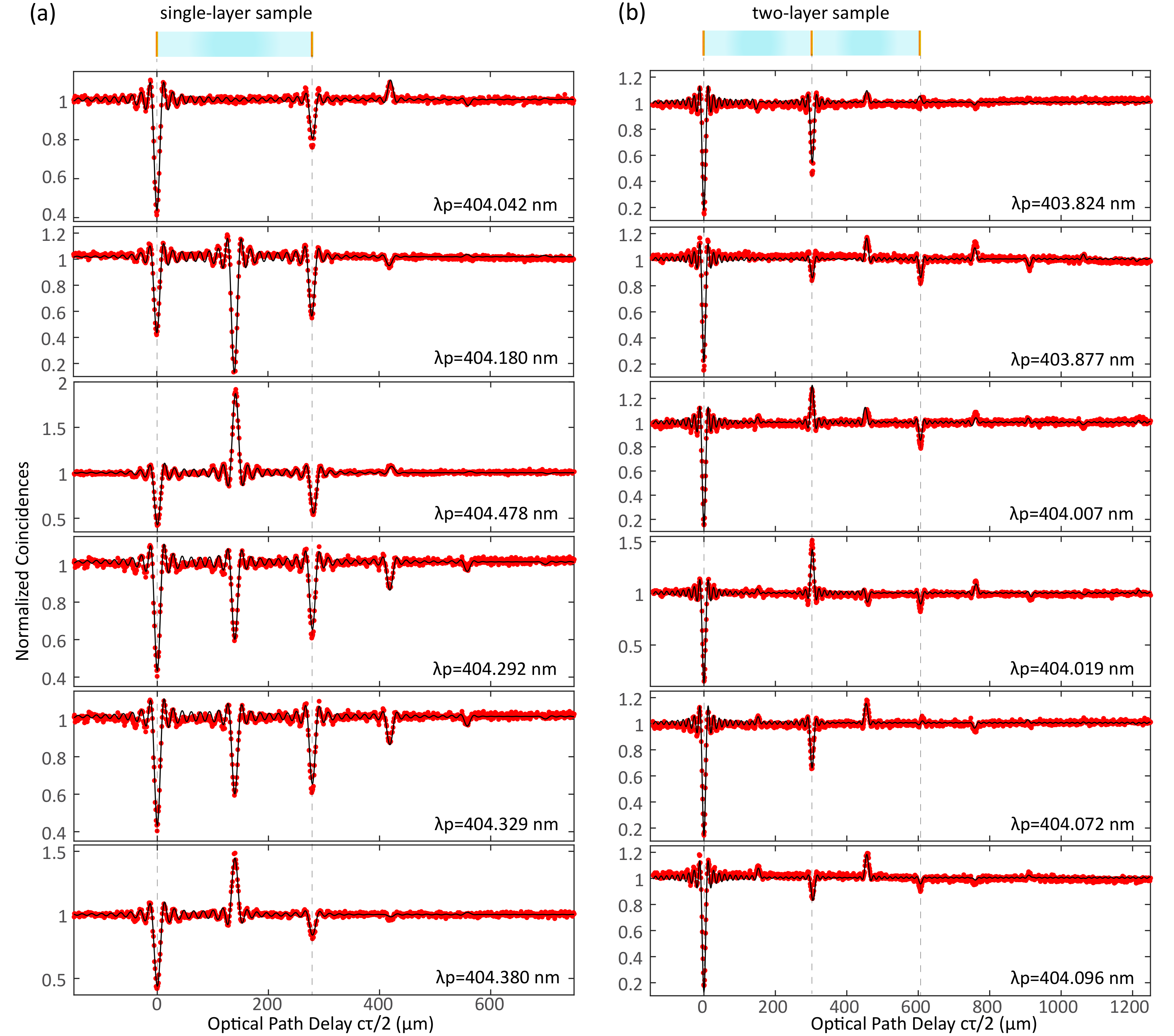
It is of interest to illustrate how our approach operates in the context of the particular peak/dip composition exhibited by the QOCT interferogram. Note that our measurements are realized by tuning the pump laser wavelength to particular values, selected to yield a peak, dip, or no artifact as predicted from the sign and amplitude of the function (with ) in the visibility parameters Eq. (II.2). The argument of the cosine function depends on the time taken by the signal photon to travel between the two interfaces responsible for creating the artifact; thus, the cosine function period depends on the distance between them. Since each artifact is created by two features (interface-interface, interface-echo, echo-echo) with a well-defined distance between them, it has its own cosine function that defines its shape for a given pump wavelength. This means that we can target a specific artifact by choosing the corresponding cosine function for pump wavelength tuning, see Fig. 6. We have used such an approach to generate a set of interferograms with different shapes for the same sample. As a result, we are able to test whether for a given sample our algorithm gives the same parameters for different input wavelengths, as the underlying sample morphology is the same.
Fig. 7(a) shows the resulting interferograms for a two-interface sample upon changing the target artifact created by the front and back surfaces of the sample. For example, the zero value of the cosine function at nm yields an artifact with zero amplitude, while a minimum in the cosine function at nm results in the dip with the largest visibility possible, and so on.
For a three-interface sample, the complexity of the signal increases, see Fig. 7(b). There are more artifacts present in the interferogram. For this case, we decided to target also the artifact associated with the front and back surfaces. The situation is more complex than for the single-layer case because the artifact overlaps with the dip corresponding to the middle interface. While the corresponding cosine function predicts a suppressed artifact for 404.096 nm, the interferogram for that wavelength is not flat even though the artifact amplitude is zero. The net dip comes from the contribution of the middle interface.
The Genetic Algorithm was programmed to estimate the width of each layer and the reflectivities of the corresponding interfaces by increasing, in each epoch, the number of layers that the unknown sample could have. For each guess of , the fitness value was retained and used as a figure of merit for the search procedure. The GA is initially given a guess and starts by assuming that the sample is single-layered, , and the optimization calculates a fitness value for this case. Next, the GA assumes a two-layer sample; i.e. , and calculates its fitness value. The procedure is repeated with increasing values of until a minimal fitness value is obtained. The best set of parameters corresponds to the case of layers for which the reconstructed interferogram best matches the experimental signal. Note that at the step of this implementation in which we assume interfaces, we set the values of the first reflectivities. While this is meant as a proof-of-principle demonstration, the possibility of for example only setting the values of the reflectivities which could be amenable to direct experimental determination is left for future analysis (see also the discussion in the Supplemental Material). As previously stated, in each step of the searching GA the QOCT interferogram is evaluated from the fitting parameters, which assumes a perfect monochromatic pump beam, i.e. with a zero SPDC pump spectral width, and that the generated photon pairs are centered around 808 nm with a width of 40 nm.
Fig. 7 shows how the reconstructed interferogram matches the experimental data after the GA has ended its search. The results for the single-layer sample are presented in Fig. 7 (a) while the results for the two-layer sample are shown in Fig. 7 (b). As seen from the plot, the reconstructed interferograms are in excellent agreement with the experimental traces, for both cases. In particular, for the case of the single-layer sample, the artifact can be clearly identified by changing the central wavelength that causes it to flip from a dip to a peak. This behavior, however, becomes problematic for a sample with a higher number of layers. For instance, in the case of the two-layer sample, the artifact produced by the front and back surfaces indeed changes from a dip to a peak when the pump wavelength is changed. However, it overlaps with the signal produced by the middle surface. As a consequence, simply filtering the signals that change their behavior as the pump wavelength is varied could potentially remove structures associated with real interfaces.
| Wavelength (nm) | (m) | |
|---|---|---|
| 404.036 | 185.227 | 0.896 |
| 404.042 | 184.566 | 0.916 |
| 404.180 | 184.801 | 0.876 |
| 404.292 | 184.826 | 0.891 |
| 404.329 | 184.705 | 0.946 |
| 404.380 | 185.091 | 0.942 |
| 404.478 | 186.278 | 0.883 |
| 185.213 | 0.907 |
| Wavel. (nm) | (m) | (m) | (m) | |
|---|---|---|---|---|
| 403.824 | 199.162 | 1.844 | 202.453 | 0.933 |
| 403.877 | 199.118 | 0.064 | 203.334 | 0.879 |
| 404.007 | 198.093 | 3.288 | 200.960 | 0.907 |
| 404.019 | 197.494 | 1.302 | 203.058 | 0.974 |
| 404.072 | 200.731 | 1.985 | 199.886 | 0.889 |
| 404.096 | 202.990 | 2.171 | 196.822 | 0.899 |
| 199.598 | 1.775 | 201.086 | 0.914 |
The optimal parameters found for both the single- and two-layer samples are summarized in Tables 3 and 2. Note that because the two-layer sample is built from two coverslips pressed together, our GA treats it as a four-interface sample, with an air gap between the second and third interfaces, leading to three distances and four reflectivities. We have provided the algorithm with the value of the reflectivity of the first interface (in the case of the 1-layer sample), and the reflectivities for the first three interfaces (in the case of the 2-layer sample), so that in both cases the algorithm is left to find a value for the last reflectivity. The algorithm predicts well the distances, although there is a larger fluctuation in the case of the air gap thickness. Additionally, we note that the reflectivity values of the last interface predicted by the algorithm are in all cases reasonably close to the nominal values. We ascribe the variations observed in the recovered parameters to the presence of noise or fluctuations in the system. For an additional discussion on the determination of the morphology of more complex samples and the effect of noise, please see the Supplemental Material.
Note that the width of our HOM dips is around m which is significantly wider than the width of the airgap m. While we cannot resolve two dips separated by such a short distance, the airgap has an effect on the reflectivities of the second and third interfaces (adjacent to the airgap), which in turn affects the dip and artifact visibilities of the interferogram as a whole. In this manner, the airgap may have an effect on the overall interferogram beyond the presence of two nearly-coincident dips which appear as a single dip in the experimental interferograms.
We point out that the experimental results presented in this paper benefit from the usual factor of improvement in axial resolution for QOCT as compared to an equivalent classical apparatus (OCT) Abouraddy_2002. In addition, it is known that for the case of a two-photon state which exhibits strict spectral anti-correlations, even-order (in particular quadratic) dispersion effects are suppressed. Such spectral anti-correlation is ensured by the use of a narrow-linewidth continuous wave laser as SPDC pump, which is indeed the case in our experiment (the linewidth of our pump laser is kHz). Thus, our experimental results benefit from quadratic dispersion cancellation.
IV Conclusions
We have presented a new, more complete model for Quantum Optical Coherence Tomography (QOCT) which accounts for the effects of real interfaces, artifacts, echoes, as well as the superposition of all these. A thorough understanding of these structures can give richer information beyond the separations between the inner interfaces within a multilayer sample. We have changed the paradigm and transitioned from suppressing artifacts to inferring the source morphology giving rise to a given interferogram, fully taking into account all artifacts and multiple reflections. Solely removing peaks or dips from the interferogram can be a naive approach as the morphology of the sample is generally unknown and artifact removal can be counterproductive since the technique comes with the risk of information loss.
Our new model exposes the complexity of the QOCT interferogram arising from the quantum nature of the source, which is affected by multiple reflections within the sample. While artifacts have been previously identified, echoes and echo-induced artifacts, as well as their possible superposition on other peaks or dips had not been reported. We have experimentally demonstrated that a given artifact can be effectively removed from the signal by tuning the pump frequency and consequently shaping its visibility to extinction. Echoes, on the other hand, survive the process and contribute to the appearance of intricate structures in the interferogram. The importance of our genetic algorithm thus lies in its ability to identify with plausibility the number of layers in a sample, as well as intra-interface distances and interface reflectivities. With further upgrades, our approach presented here could bring the possibility of monitoring small-scale light-sensitive biological entities such as living cells and bacteria without introducing optical damage.
Acknowledgments
S.B. acknowledges funding by the Natural Sciences and Engineering Research Council of Canada (NSERC) through its Discovery Grant, funding and advisory support provided by Alberta Innovates through the Accelerating Innovations into CarE (AICE) – Concepts Program, and support from Alberta Innovates and NSERC through Advance Grant. This project is funded [in part] by the Government of Canada. Ce projet est financé [en partie] par le gouvernement du Canada. AU acknowledges Consejo Nacional de Ciencia y Tecnología (CF-2019-217559), PAPIIT-UNAM (IN103521), and AFOSR (FA9550-21-1-0147). VS acknowledges the support from Alberta Innovates grant.
References
- (1) C. L. Degen, F. Reinhard, and P. Cappellaro, “Quantum sensing,” Rev. Mod. Phys., vol. 89, p. 035002, Jul 2017.
- (2) J. P. Dowling and K. P. Seshadreesan, “Quantum optical technologies for metrology, sensing, and imaging,” Journal of Lightwave Technology, vol. 33, no. 12, pp. 2359–2370, 2015.
- (3) S. Barzanjeh, S. Guha, C. Weedbrook, D. Vitali, J. H. Shapiro, and S. Pirandola, “Microwave quantum illumination,” Phys. Rev. Lett., vol. 114, p. 080503, Feb 2015.
- (4) S. Pirandola, B. R. Bardhan, T. Gehring, C. Weedbrook, and S. Lloyd, “Advances in photonic quantum sensing,” Nature Photonics, vol. 12, pp. 724–733, Dec 2018.
- (5) S. Barzanjeh, S. Pirandola, D. Vitali, and J. M. Fink, “Microwave quantum illumination using a digital receiver,” Science Advances, vol. 6, no. 19, p. eabb0451, 2020.
- (6) D. Braun, G. Adesso, F. Benatti, R. Floreanini, U. Marzolino, M. W. Mitchell, and S. Pirandola, “Quantum-enhanced measurements without entanglement,” Rev. Mod. Phys., vol. 90, p. 035006, Sep 2018.
- (7) V. Giovannetti, S. Lloyd, and L. Maccone, “Advances in quantum metrology,” Nature Photonics, vol. 5, pp. 222–229, Apr 2011.
- (8) S. Ahmadi, E. Saglamyurek, S. Barzanjeh, and V. Salari, High-contrast interaction-free quantum imaging method. Phys. Rev. A. 107, 032611, March 2023.
- (9) V. Salari, D. Paneru, E. Saglamyurek, M. Ghadimi, M. Abdar, M. Rezaee, M. Aslani, S. Barzanjeh, and E. Karimi, Quantum face recognition protocol with ghost imaging. Scientific Reports. 13, 2401, Feb 2023.
- (10) A. F. Abouraddy, M. B. Nasr, B. E. A. Saleh, A. V. Sergienko, and M. C. Teich, “Quantum-optical coherence tomography with dispersion cancellation,” Phys. Rev. A, vol. 65, p. 053817, May 2002.
- (11) M. B. Nasr, D. P. Goode, N. Nguyen, G. Rong, L. Yang, B. M. Reinhard, B. E. Saleh, and M. C. Teich, “Quantum optical coherence tomography of a biological sample,” Optics Communications, vol. 282, no. 6, pp. 1154–1159, 2009.
- (12) M. C. Teich, B. E. A. Saleh, F. N. C. Wong, and J. H. Shapiro, “Variations on the theme of quantum optical coherence tomography: a review,” Quantum Information Processing, vol. 11, pp. 903–923, Aug 2012.
- (13) D. Lopez-Mago and L. Novotny, “Quantum-optical coherence tomography with collinear entangled photons,” Opt. Lett., vol. 37, pp. 4077–4079, Oct 2012.
- (14) J. Lavoie, R. Kaltenbaek, and K. J. Resch, “Quantum-optical coherence tomography with classical light,” Opt. Express, vol. 17, pp. 3818–3826, Mar 2009.
- (15) P. Y. Graciano, A. M. Martínez, D. Lopez-Mago, G. Castro-Olvera, M. Rosete-Aguilar, J. Garduño-Mejía, R. R. Alarcón, H. C. Ramírez, and A. B. U’Ren, “Interference effects in quantum-optical coherence tomography using spectrally engineered photon pairs,” Scientific Reports, vol. 9, no. 1, 2019.
- (16) F. Bouchard, A. Sit, Y. Zhang, R. Fickler, F. M. Miatto, Y. Yao, F. Sciarrino, and E. Karimi, “Two-photon interference: the hong–ou–mandel effect,” Reports on Progress in Physics, vol. 84, p. 012402, dec 2020.
- (17) M. B. Nasr, D. P. Goode, N. Nguyen, G. Rong, L. Yang, B. M. Reinhard, B. E. Saleh, and M. C. Teich, “Quantum optical coherence tomography of a biological sample,” Optics Communications, vol. 282, no. 6, p. 1154–1159, 2009.
- (18) P. Yepiz-Graciano, Z. Ibarra-Borja, R. R. Alarcón, G. Gutiérrez-Torres, H. Cruz-Ramírez, D. Lopez-Mago, and A. B. U’Ren, “Quantum-optical coherence microscopy for bio-imaging applications,” May 2022.
- (19) Z. Ibarra-Borja, C. Sevilla-Gutiérrez, R. Ramírez-Alarcón, H. Cruz-Ramírez, and A. B. U’Ren, “Experimental demonstration of full-field quantum optical coherence tomography,” Photon. Res., vol. 8, pp. 51–56, Jan 2020.
- (20) B. Ndagano, H. Defienne, D. Branford, Y. D. Shah, A. Lyons, N. Westerberg, E. M. Gauger, and D. Faccio, “Quantum microscopy based on hong–ou–mandel interference,” Nature Photonics, vol. 16, no. 5, p. 384–389, 2022.
- (21) S. M. Kolenderska, F. Vanholsbeeck, and P. Kolenderski, “Fourier domain quantum optical coherence tomography,” Opt. Express, vol. 28, pp. 29576–29589, Sep 2020.
- (22) S. M. Kolenderska and M. Szkulmowski, “Artefact-removal algorithms for fourier domain quantum optical coherence tomography,” Scientific Reports, vol. 11, p. 18585, Sep 2021.
- (23) T. Liu, Y. Sun, and X. Zhang, “Denoising of fourier domain quantum optical coherence tomography spectrums based on deep-learning methods,” Opt. Continuum, vol. 1, pp. 705–717, Apr 2022.
- (24) M. C. T. Bahaa E. A. Saleh, Fundamentals of Photonics. Wiley-Interscience, 2007.
- (25) Multi-Photon Quantum Interference. Springer US, 2007.
- (26) P. Y. Graciano, A. M. A. Martínez, D. Lopez-Mago, G. Castro-Olvera, M. Rosete-Aguilar, J. Garduño-Mejía, R. R. Alarcón, H. C. Ramírez, and A. B. U’Ren, “Interference effects in quantum-optical coherence tomography using spectrally engineered photon pairs,” Scientific Reports, vol. 9, p. 8954, Jun 2019.
- (27) O. E. David and I. Greental, “Genetic algorithms for evolving deep neural networks,” in Proceedings of the Companion Publication of the 2014 Annual Conference on Genetic and Evolutionary Computation, GECCO Comp ’14, (New York, NY, USA), p. 1451–1452, Association for Computing Machinery, 2014.
- (28) L. Chambers, The Practical Handbook of Genetic Algorithms. Chapman & Hall/CRC, 2001.
- (29) S. N. Pawar and R. S. Bichkar, “Genetic algorithm with variable length chromosomes for network intrusion detection,” International Journal of Automation and Computing, vol. 12, pp. 337–342, Jun 2015.
- (30) O. S. Heavens, “Optical properties of thin films,” Reports on Progress in Physics, vol. 23, p. 1, jan 1960.
- (31) Z. H. Mohammed, “The fresnel coefficient of thin film multilayer using transfer matrix method tmm,” IOP Conference Series: Materials Science and Engineering, vol. 518, p. 032026, may 2019.
Supplementary Materials
In this supplemental material section, we discuss the power of our genetic algorithm for the determination of the sample morphology, particularly providing an example of a more complex five-interface sample. This example involves an interferogram computed from our model (rather than obtained experimentally) so that there is a complete absence of noise.
An illustrative morphology determination example
We consider a sample with dielectric interfaces each of which is assumed to be well-described as lossless, and we separately consider the effects of a metallic layer through a loss matrix. Each interface is described by two complex-valued reflectivities (forward and backward) as well as two complex-valued transmissivities (forward and backward). This gives 4 complex-valued parameters or 8 real-valued parameters per interface. Now, for a lossless interface (between media and ) there are 4 constraints on these 8 parameters: , , , and . This leaves 4 effective real-valued parameters per interface. For the last interface, it is only the forward reflectivity that can have an effect on the QOCT interferogram, so this last interface is described by a single effective parameter. For the interfaces, we then have effective, real-valued parameters. In addition, for each of the transmissive segments (corresponding to interfaces) we have one optical distance and one loss parameter, yielding effective parameters. In total, for interfaces we then have effective real-valued parameters. Thus, the complexity of the problem could be considered to scale with as .
In principle, the problem of determining the sample morphology from the interferogram corresponds to the determination of these real-valued parameters from the interferogram. The visibility of each of the features (dip or peak) in the interferogram provides a constraint (an equation) so that if the number of equations can be made equal to the number of parameters, we may be in a position to extract the values of all parameters. Let us consider as an example the case of 2 interfaces (1 layer). In this case, in the interferogram we may observe features corresponding to: i) the two dips, ii) the artifact between the two interfaces, and iii) the echoes as well as artifacts involving echoes. Some of these features involve multiple contributing processes as described in the main text, for example, the second dip is overlapped with the artifact between the first interface and the first echo. If we consider the two dips and the first artifact, that only gives us 3 constraints, while the number of effective parameters is . If we consider in addition the first echo as well as the artifact between the second interface and the first echo, that gives us 5 constraints, still short of the 7 parameters. In the absence of noise so that we may reliably observe the second echo as well as the artifact between the first two echoes, that gives us the 7 constraints that we need in order to extract all 7 parameters. The optimization carried out by our GA algorithm can be thought of as being equivalent to solving a number of coupled equations derived from each of the interferogram features as described above. Note also that actually solving such a system of equations for an unknown sample may not be practical, as it would hinge on being able to fully identify each of the interferogram features which as will be shown below for a specific example can become extremely challenging.
| Nominal | Retrieved | |
| (m) | 90 | 91.116 |
| (m) | 110 | 107.440 |
| (m) | 150 | 152.100 |
| (m) | 250 | 249.730 |
| 0.1 | - | |
| 0.1 | 0.096 | |
| 0.1 | 0.095 | |
| 0.5 | 0.506 | |
| 0.9 | 0.901 |
In an actual experiment with noise and other experimental imperfections, it becomes rapidly difficult to resolve progressively smaller features from the noise. We may conclude that while for an ideal (noiseless) situation we could be in a position to unambiguously determine all effective parameters from the interferogram, in an actual experiment this will most likely not be the case. To illustrate this discussion, we present in Figure 8 an interferogram (blue line) calculated using our QOCT model for a particular five-interface losssless sample with assumed (nominal) parameter values shown in table 3. Note that for such a complex sample it becomes difficult to identify particular features in the interferogram, a challenge which becomes more acute as the number of interfaces is increased. We now take this interferogram as input for our algorithm, which then outputs both a fitted interferogram (red line) and provides values for the retrieved parameters. It is notable that in this case, because there is a complete absence of noise (the interferogram is derived from our model and not from the experiment), the quality of the fit is excellent and the retrieved parameters match closely the nominal ones. This highlights the power of our GA approach for the determination of the morphology.