Formatting Instructions For NeurIPS 2022

David S. Hippocampus Thanks: Use footnote for providing further information about author (webpage, alternative address)—not for acknowledging funding agencies. Affiliation: Department of Computer Science Affiliation: Cranberry-Lemon University Affiliation: Pittsburgh, PA 15213 Email: hippo@cs.cranberry-lemon.edu

Abstract

The abstract paragraph should be indented $\nicefrac{{1}}{{2}}$ inch (3 picas) on both the left- and right-hand margins. Use 10 point type, with a vertical spacing (leading) of 11 points. The word Abstract must be centered, bold, and in point size 12. Two line spaces precede the abstract. The abstract must be limited to one paragraph.

1 Introduction

Deep reinforcement learning has achieved great success in a wide range of challenging environments such as Atari games (26; 4; 19) or continuous control tasks (32; 33). However, in stark contrast with this trend, applying RL to real-world applications remains a great challenge. In most real-world settings, there could be variations in environmental factors, such as changing terrains in robotic tasks, fluctuated bandwidth in congestion control, and dynamic traffic patterns in autonomous driving. We refer to such environment factors as situation or context. The changes in context are not neglectable since context usually has a substantial impact on transition and reward functions. When the context is fixed and known to us, the problem is stationary and easier to solve. However, in most realistic settings, the context is usually dynamic within an episode and unknown to us at test time. Therefore, detecting and adapting to variations in context is very important for RL agents to make a real impact in a wide range of real-world applications.

Refer to caption — Figure 1: A typical trace of network available bandwidth. The trace can be approximately divided into several segments of different length $g^{i}$ , for $i\in\{1,2,\cdots,6\}$ . The network condition changes abruptly at the end of each \lisegment, while in each segment the network condition stays stable.

In real-world environments with varied unknown contexts, we find a typical evolving context pattern particularly interesting. The context $c$ usually stays the same for a stochastic period until it changes abruptly and unpredictably into another context value $c^{\prime}$ which is sampled i.i.d. from some prior context distribution. What’s more, we usually do not have access to context $c$ directly but instead have access to some noisy observation $x_{t}$ sampled from some distribution $p(x_{t}|c)$ only at training time \li(e.g., as auxiliary information from the simulator). We take fluctuated bandwidth in congestion control as an example. In Figure 1, we show a typical trace of network available bandwidth. The fluctuated bandwidth is usually modeled by multiple non-overlapping segments (1; 39). Within each segment, the network condition is stationary, and thus the bandwidth approximately follows the same distribution. At the end of a segment, the network condition changes, and the bandwidth changes abruptly into another distribution. Here the context $c$ represents the parameters that determine the distribution of fluctuated bandwidth (network condition), while the observations $x_{t}$ represents the observed bandwidth which follows the above distribution $p(x_{t}|c)$ . While the contexts $c$ are piecewise-stable, there could be slight variations in $x_{t}$ within each segment. This piecewise-stable pattern of context dynamics is of particular interest to us since it can capture a wide range of stochastic context processes in real-world applications, such as changing terrains in robotic tasks and fluctuating bandwidth in congestion control. Since the change in context is abrupt and unpredictable, we cannot predict the future context in advance. The best we can do is detect and adapt to changes when they happen.

Although adaptation to varied unknown contexts has been studied under non-stationary RL and meta RL, few existing works look into piecewise stable context with abrupt changes within an episode. Most works in meta RL as task inference (30; 41; 40; 29) and some works in non-stationary RL (6; 7; 37) assume the context stays the same for the whole episode and infer the context based on the entire episode (c.f. Figure 2(a)), therefore cannot quickly adapt to context changes within an episode. Other works on non-stationary RL assume intra-episode context changes and model $c_{t}$ at each time step, but few study the piecewise-stable context as we do. 27 directly predict the context and thus cannot capture the prior that the context tends to stay the same for a stochastic period. 12; 31 model Markovian discrete context for each time step (c.f. Figure 2(b)), therefore failing to model the non-markov property of context and the prior over context segment length in our setting. Compared with existing works, our setting is distinctive since the segment structure is latent to us (c.f. Figure 2(c)). Therefore, the unique challenge in our setting is that we need to infer the segment structure, which can be further leveraged to infer belief context by only incorporating the relevant observed data in the current segment.

\li

This paper studies how to infer segment structure to detect abrupt context changes and infer belief context accordingly to adapt to the piecewise-stable context in RL environments. We first introduce latent situational MDP which models RL environments with the stochastic situation/context process (Section 2). Then, we introduce how to infer the belief context from observed data. To address the challenge above, we propose to infer context segment structure and belief context jointly from observed data (Section 3.1). Then we augment the state with inferred belief context so that the RL agent can automatically trade-off between acting optimally conditioned on inferred context and gathering more information about the current context (Section 3.2). Finally, we combine the training objectives for RL and inference and present all the details for our proposed deep RL algorithm (Section 3.3). We evaluate our algorithm on a gridworld environment with dynamic goals and MuJoCo tasks (36) with varied contexts. Experiments demonstrate that our algorithm can quickly detect and adapt to abrupt changes in piece-wise stable contexts and outperform existing methods(Section ).

Our contributions can be listed as follows:

•

We introduce latent situational MDP with piecewise-stable context, which can capture a wide range of real-world applications (Section 2).
•

We propose SeCBAD, an adaptive deep RL method for non-stationary environments with piecewise-stable context. Our method can infer the context segment structure and the belief context accordingly from observed data, which can be leveraged to detect and adapt to context changes (Section 3).
•

Experiments on a gridworld environment and Mujuco tasks with piecewise-stable context demonstrate that our method can quickly detect and adapt to abrupt context changes and outperform existing methods (Section ).

2 Problem Formulation

In this section, we define a latent situational Markov Decision Process (LS-MDP) as a tuple $M=(\mathcal{S},\mathcal{A},\mathcal{C},\mathcal{X},G,T,R,\gamma)$ , where $\mathcal{S}$ is the set of states, $\mathcal{A}$ is the set of actions, and $\gamma\in(0,1]$ is the discount factor. To formulate the variations in environment factors, we introduce $\mathcal{C}$ , the set of latent contexts, and $\mathcal{X}$ , the set of observable contexts. $\mathcal{C}$ refers to the set of underlying hidden contexts that contains all necessary information but are left unobservable to the agent, while $\mathcal{X}$ refers to the set of contexts with only partial information. $G$ refers to the segment length which will be described in detail in the next paragraph. $\mathcal{X}$ are observable only during training and unobservable during deployment. In an example environment setting where a robot walking over changing terrain, $\mathcal{C}$ represents the terrain features containing perfect information, and $\mathcal{X}$ represents noisy and imperfect information like mechanical metrics of the current step from virtual sensors in a simulator and thus is only accessible during training.

In our setting, we focus on the case where the environmental changes are abrupt and irregular, \liin contrast to the smoothly changing assumption on context/task in existing works in non-stationary RL (6; 7). To better model the generative process of the contexts, we introduce the segment length $G$ . Each episode is composed of several stationary segments \liwith different segment lengths. For the ease of notation, we also introduce $G_{t}$ , which measures the length of the current segment up to time step $t$ . Then, the generative process can be described as follows: at the beginning of the $h$ -th segment, the environment samples $G^{h}\sim p_{G}(G)$ and $c^{h}\sim p_{c}(c)$ from \liprior distributions $p_{G}$ and $p_{c}$ . Then, in the next $G^{h}$ steps, the latent context $c^{h}$ remains unchanged. For each time step $t$ in this segment, the current segment length accumulates as $G_{t}=G_{t-1}+1$ (we define $G_{t}=1$ for the first time step in this segment), and the current latent context satisfies that $c_{t}=c^{h}$ . The agent can observe $x_{t}\sim p(x_{t}|c_{t})$ for each time step if during training. The stationarity lasts until the end of the current segment, then the environment resamples $G^{h+1}$ and $c^{h+1}$ , and the process repeats. \liWe show two examples of graphical models of our setting given different $G_{t}$ in Figure 2(c).

The transition function $T:p(s_{t+1}|s_{t},a_{t},c^{h})$ and the reward function $R:p(r_{t}|s_{t},a_{t},c^{h})$ are all conditioned on current latent context $c^{h}$ . Therefore the changes in $\mathcal{C}$ lead to the changes in transition and reward functions. \liAt test time, $\mathcal{X}$ is no longer accessible, so we need to infer context changes from observed transitions and rewards. Since the latent context $\mathcal{C}$ remains unobservable and changes silently, the environment is no longer stationary for the agents. To act optimally, it is important to keep track of the environment to recognize changes in time, and rapidly adapt to those changes.

3 Methodology

In this section, we present our Segmented Context Belief Augmented Deep (SeCBAD) RL method and elaborate on how SeCBAD solves the challenges discussed above. Our method consists of two main components:

•

Joint inference of the belief distribution over the latent context and the segment structure from observed data.
•

Policy optimization with inferred belief context under the belief MDP framework.

We first introduce the latent context inference part in Section 3.1, especially how to infer the segment structure jointly with belief context and leverage the segment structure to remove irrelevant observed data. \liAfter the belief context is approximated, it is then incorporated into the state as the input of the policy. We detail the policy optimization part under the belief MDP framework in Section 3.2. And finally, in Section 3.3, we describe how these parts constitute a practical algorithm.

3.1 Joint Inference for Belief Context and Segment Structure

In this part, we perform joint inference over latent context $c_{t}$ and current segment length $G_{t}$ from observed trajectory $\tau_{1:t}$ , so as to remove irrelevant data in $\tau_{1:t}$ for belief context inference. This can be formally expressed by the following equation:

p(c_{t},G_{t}|\tau_{1:t})=p(c^{t-G_{t}+1:t}|G_{t},\tau_{t-G_{t}:t})p(G_{t}|\tau_{1:t})

(1)

where $\tau_{t_{0}:t}=(s_{t_{0}},a_{t_{0}},r_{t_{0}}\cdots,s_{t-1},a_{t-1},r_{t-1},s_{t})$ ¹¹ 1 This definition makes $\tau_{t-G_{t}:t}$ only contain observed data that belong to the current segment., and $c^{t-G_{t}+1:t}$ refers to the latent context for the whole segment from $t-G_{t}+1$ to $t$ . In Equation 1, we separately estimate the posterior $p(c^{t-G_{t}+1:t}|G_{t},\tau_{t-G_{t}:t})$ of latent context given known segment structure $G_{t}$ , and the posterior of segment length $p(G_{t}|\tau_{1:t})$ .

3.1.1 Approximate Inference for Latent Context under Known Segment Structure

In this part, we focus on estimating $p(c^{t-G_{t}+1:t}|G_{t},\tau_{t-G_{t}:t})$ , which is the posterior of the latent context under known segment structure $G_{t}$ . We use the variational inference framework to approximate the true posterior. To be specific, we use an posterior inference network $q_{\phi}$ to infer the belief context in segment $[t-G_{t}+1:t]$ : $q_{\phi}(c^{t-G_{t}+1:t}|G_{t},\tau_{t-G_{t}:t})$ . The variational lower bound for the log-likelihood of the current segment is given by:

		$\displaystyle\quad\log p(\tau^{X}_{t-G_{t}:t}\|a_{t-G_{t}:t-1},s_{t-G_{t}},G_{t})$
		$\displaystyle\geq\mathbb{E}_{q_{\phi}(c^{t-G_{t}+1:t}\|G_{t},\tau_{t-G_{t}:t})}\left[\log p_{\theta}(\tau^{X}_{t-G_{t}:t}\|G_{t},c^{t-G_{t}+1:t},a_{t-G_{t}:t-1},s_{t-G_{t}})\right]$
		$\displaystyle\quad\quad\quad\quad\quad\quad\quad\quad\quad-\mathbf{D}_{KL}(q_{\phi}(c^{t-G_{t}+1:t}\|G_{t},\tau_{t-G_{t}:t})\\|p(c^{t-G_{t}+1:t}))\coloneqq\mathcal{J}_{Model}^{t}(G_{t})$		(2)

where $p_{\theta}$ denotes the decoder and $\tau^{X}_{t-G_{t}:t}=(\tau_{t-G_{t}:t},x_{t-G_{t}+1:t})$ . For the detailed derivation, please see Appendix A.1.

The reconstruction term of Equation 3.1.1 can be factorized as:

		$\displaystyle\quad\log p_{\theta}(\tau^{X}_{t-G_{t}:t}\|G_{t},c^{t-G_{t}+1:t},a_{t-G_{t}:t-1},s_{t-G_{t}})$
		$\displaystyle=\sum_{i=t-G_{t}+1}^{t}\log p_{\theta}(x_{i},s_{i},r_{i-1}\|G_{t},c^{t-G_{t}+1:t},s_{i-1},a_{i-1})$		(3)

which is the sum of log-probablity of transitions under context sampled from $q_{\phi}$ . The term $\mathbf{D}_{KL}(q_{\phi}||p)$ is the KL-divergence between our variational posterior $q_{\phi}$ and the prior over the belief context. For the prior $p(c^{t-G_{t}+1:t})$ , we use previous posterior at timestep $t-1$ if the context remains unchanged at timestep $t$ , or $\mathcal{N}(0,I)$ otherwise.

Unlike most previous methods which assume invariant context within an episode or markovian context at each time step, our method 1) takes only observed data within current segment $\tau_{t-G_{t}:t}$ as input for encoder $q_{\phi}$ , 2) reconstructs only data within current segment $\tau^{X}_{t-G_{t}:t}$ at the output for decoder $\log p_{\theta}$ . Our method is naturally motivated by the piecewise-stable assumption on context dynamics. By removing irrelevant data outside the current segment \pushithat are generated by past unassociated context, our method can estimate the current latent context more accurately.

3.1.2 Iterative Inference for the Segment Length

In this part, we focus on estimating $p(G_{t}|\tau_{1:t})$ , which is the posterior for current segment length, given $p(c^{h}|\tau_{t-G_{t}:t})$ , the posterior of context under given segment structure. To compute this posterior distribution, we first compute the joint distribution $p(G_{t},\tau_{1:t})$ recursively based on $p(G_{t-1},\tau_{1:t-1})$ as follows²² 2 For notation simplicity, we omit the condition $G_{t}=i$ in the term $p(s_{t},a_{t-1},r_{t-1}|\tau_{t-i:t-1})$ , i.e. $t-i$ is the start of the segment. :

\displaystyle p(G_{t}=i,\tau_{1:t})

\displaystyle=\sum_{k=1}^{t-1}p(G_{t-1}=k,\tau_{1:t-1})\cdot p(G_{t}=i|G_{t-1}=k)\cdot p(s_{t},a_{t-1},r_{t-1}|\tau_{t-i:t-1})

(4)

The three major components in Equation 4 in turn are the previous joint distribution, the evolution prior, and the observation probability. The previous joint distribution is iteratively provided at the beginning of each time step. The evolution prior $p(G_{t}=i|G_{t-1}=k)$ measures the prior knowledge on the segment length $G_{t}$ given the segment length of the previous time step $G_{t-1}=k$ , where either $G_{t}=G_{t-1}+1$ or $G_{t}=1$ holds.

As for the observation probability which is the third term of Equation 4, it measures how likely the observations show up given the history of the segment. To be specific, we have ³³ 3 In Equation 5, $K=p(a_{t-1}|s_{t-1})$ is a constant with respect to $i$ and has no impact on the posterior $p(G_{t}=i|\tau_{1:t})$ .

\displaystyle p(s_{t},a_{t-1},r_{t-1}|\tau_{t-i:t-1})

\displaystyle=K\mathbb{E}_{p(c^{t-i+1:t}|G_{t}=i,\tau_{t-i:t-1})}\Big[p(s_{t},r_{t-1}|s_{t-1},a_{t-1},c^{t-i+1:t})\Big]

(5)

In Equation 5, the term $p(s_{t},r_{t-1}|s_{t-1},a_{t-1},c^{t-i+1:t})$ estimates the data likelihood for the next state-reward pair, where $c$ is drawn from the posterior distribution given the data in the segment before timestep $t$ . To compute the RHS of Equation 5, we sample from $q_{\phi}(c^{t-i+1:t-1}|G_{t}=i,\tau_{t-i:t-1})$ ⁴⁴ 4 When $i\geq 2$ , we can use the belief $q_{\phi}(c^{t-i+1:t-1}|G_{t-1}=i-1,\tau_{t-i:t-1})$ to approximate the posterior $p(c^{t-i+1:t}|G_{t}=i,\tau_{t-i:t-1})$ . For the case where $i=1$ , the posterior distribution $p(c^{t-i+1:t}|G_{t}=i,\tau_{t-i:t-1})$ is actually the prior distribution $p_{c}(c)=\mathcal{N}(0,I)$ , and we can sample $c$ from the prior distribution. which is the belief context inferred from the whole history of the segment before timestep $t$ , and use the sampled $c$ the decoder to compute the data likelihood.

Given the joint distribution, the posterior distribution of $G_{t}$ can be derived as

p(G_{t}=i|\tau_{1:t})=\frac{p(G_{t}=i,\tau_{1:t})}{\sum_{l}p(G_{t}=l,\tau_{1:t})}

(6)

We can also incorporate observable contexts $x$ in the observation probability to improve accuracy during training. See Appendix A.3 for more details.

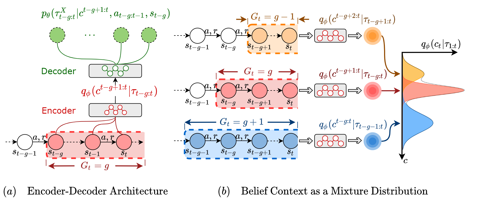
3.1.3 Belief Context as a Mixture Distribution

Given inferred posterior of $G_{t}$ in Section 3.1.2, the belief of the latent context at time step $t$ can be derived as

b_{t}(c)=q_{\phi}(c_{t}|\tau_{1:t})=\sum_{g_{t}}q_{\phi}(c^{t-g_{t}+1:t}|G_{t}=g_{t},\tau_{t-g_{t}:t})p(G_{t}=g_{t}|\tau_{1:t})

(7)

This mixed probability of $c^{t-g_{t}+1:t}$ which has taken all possible segment structures into consideration, can now represent the current belief $b_{t}$ of the latent context $c$ .

3.2 Policy Optimization with Belief Context

Inspired by the belief MDP (21), Bayes Adaptive MDP (BAMDP) (10) \liand recent works on meta RL as task inference (41), \liwe incorporate the inferred belief context into the augmented state. At \lieach time step $t$ , the belief latent context is approximated via $q_{\phi}$ using Equation 7. Therefore, we define the augmented state as $(s,b)\in\mathcal{S}\times\mathcal{B}$ , where $\mathcal{S}$ is the same state space as in \liLS-MDP and $\mathcal{B}$ is the set of belief latent contexts. \liAccordingly, we have transition $T^{b}(s_{t+1},r_{t},b_{t+1}|s_{t},a_{t},b_{t})=p(s_{t+1},r_{t}|s_{t},a_{t},b_{t})p(b_{t+1}|s_{t},a_{t},r_{t},s_{t+1},b_{t})$ and reward $R^{b}(r_{t}|s_{t},b_{t},a_{t})$ This definition brings advantages in the sense that the information gathering and exploitation tradeoff is no longer a problem under such augmented states, since the transition and reward functions are no longer conditioned on exact $c$ . Now, the policy is defined as $\pi(a|s,b)$ a mapping from the augmented state space to the action space, and the agent’s objective is to maximize

\displaystyle\li{J_{RL}=\mathbb{E}_{s_{0},b_{0},\pi,T^{b}}\left[\sum_{t=0}^{H}\gamma^{t}R^{b}(r_{t}|s_{t},b_{t},a_{t})\right].}

(8)

3.3 Algorithm and Implementations of SeCBAD

In this section, we describe the overall algorithm and implementation details of SeCBAD. See Figure 3 for an overview of our framework. As shown in Figure 3(a), we use a GRU (8) parameterized by $\phi$ as the recurrent encoder $q_{\phi}$ , and distributions in latent context space is assumed to be diagonal Gaussians with mean and variance parameterized by $q_{\phi}$ . The decoder includes transition model $p_{\theta}(s_{t+1}|s_{t},a_{t},c)$ , reward model $p_{\theta}(r_{t}|s_{t},a_{t},c)$ and observable context model $p_{\theta}(x_{t}|c)$ . \liThe output of all the decoders are Gaussian distributions with mean parameterized by feed-forward neural networks and fixed identity covariance. Then, we estimate $p(G_{t}|\tau_{1:t})$ using $q_{\phi}$ and $p_{\theta}$ as described in Section 3.1.2. As shown in Figure 3(b), we combine the belief context based on different segment according to $p(G_{t}|\tau_{1:t})$ to get the belief $b_{t}(c)=q_{\phi}(c_{t}|\tau_{1:t})$ , where one approach is to provide a total of $t$ mean, covariance and weights as policy input. For simplicity, we choose $G_{t}^{*}$ with highest probability in $p(G_{t}|\tau_{1:t})$ and use the corresponding $q_{\phi}(c^{t-G_{t}^{*}+1:t}|\tau_{t-G_{t}^{*}:t})$ as the belief. Empirically, we find this approximation leads to little performance loss. We build our RL algorithm on the top of PPO (34) to learn the policy $\pi_{\psi}(a_{t}|s_{t},b_{t}(c))$ , where $\psi$ denotes the parameters in the actor and the critic. We use the objective described in Section 3.2 to optimize the policy.

During deployment, $q_{\phi}$ and $p_{\theta}$ are fixed. We first compute the segment posterior $p(G_{t}|\tau_{1:t})$ using encoder $q_{\phi}$ and the transition and reward model $p_{\theta}$ . Then, we estimate the belief $b_{t}(c)$ and feed it into the policy as input. For more implementation details, please refer to the Appendix A.6.

4 Related works

Our work is closely related to non-stationary RL, where the transition and reward functions may change over time. Most existing works on non-stationary RL focus on inter-episode non-stationarity (37; 6; 7; 38; 35; 3; 29; 2), some of which adopt contextual MDP as formulation (16). Recently there are some works considering intra-episode non-stationarity (31; 22; 25; 27; 12). 31 assume the latent context to be finite and Markovian, while 12 assume the latent context is Makovian and the environment can be modeled as a factored MDP. In contrast to existing works on non-stationary MDP, we assume piecewise-stable context with abrupt changes within an episode, which is more realistic and can capture a wide range of real-world applications. To rapidly adapt to dynamic context, the agent needs to continuously perform information gathering behavior. Bayesian RL (10; 41; 11) is an elegant framework to optimally tradeoff the exploration and exploitation in an unknown and stationary MDP. As a special type of Belief MDP (21), Bayes Adaptive MDP (BAMDP) (10) maintains a belief over the environment and uses this belief to augment the state. \liOur model can be viewed as a special case of belief MDP, where we only maintain belief over latent context to trade off between information gathering and exploitation. To accurately infer belief context, we adopt the variational inference, which has been adopted by many existing works in RL for task inference (30; 40; 20; 29; 41) or context inference (37; 12; 31). However, none of these methods suit our setting. \liWe perform joint inference over latent context and segment structure from observed data, so as to remove irrelevant data for more accurate belief context inference. LS-MDP can also be viewed as a special case of POMDP. Recently, progress has been made in learning the latent dynamics model (24; 23; 9; 5; 13; 17; 15; 14). Theoretically, it is possible to perform optimally only using recurrent neural networks (RNNs) like 18 since the whole history has been taken into consideration. However, it has been shown that (15) introducing more structured information will significantly enhance the performance. In this paper, we \liexploit the addtional assumption of LS-MDP to infer the context based on segment structure. The experiments show that SeCBAD can achieve better performance compared with \liexisting methods.

5 Conclusion

In this paper, we propose SeCBAD, a Segmented Context Belief Augmented Deep RL method to deal with piecewise-stable context in non-stationary environments. Piecewise-stable context is quite common in a wide range of real-world applications. Compared with existing methods, our method can automatically detect the segment structure, which reflects when the context changes abruptly. The detected segment structure can be further used to compute context belief with only relevant observed data. To the best of our knowledge, this is the first method that can model and leverage piecewise-stable context in reinforcement learning to help the agent adapt to environment change. With inferred belief context, our RL agents can quickly detect and adapt to abrupt changes in a gridwold environment and mujoco tasks with piecewise-stable context. For future work, we plan to leverage various deep learning techniques to improve SeCBAD, which includes replacing the GRU encoder by Transformer to better capture the long-term dependency in the input trajectory segment.

6 Submission of papers to NeurIPS 2022

Please read the instructions below carefully and follow them faithfully.

6.1 Style

Papers to be submitted to NeurIPS 2022 must be prepared according to the instructions presented here. Papers may only be up to nine pages long, including figures. Additional pages containing only acknowledgments and references are allowed. Papers that exceed the page limit will not be reviewed, or in any other way considered for presentation at the conference.

The margins in 2022 are the same as those in 2007, which allow for $\sim$ $15\%$ more words in the paper compared to earlier years.

Authors are required to use the NeurIPS LaTeX style files obtainable at the NeurIPS website as indicated below. Please make sure you use the current files and not previous versions. Tweaking the style files may be grounds for rejection.

6.2 Retrieval of style files

The style files for NeurIPS and other conference information are available on the World Wide Web at

http://www.neurips.cc/

The file neurips_2022.pdf contains these instructions and illustrates the various formatting requirements your NeurIPS paper must satisfy.

The only supported style file for NeurIPS 2022 is neurips_2022.sty, rewritten for LaTeX 2ε. Previous style files for LaTeX 2.09, Microsoft Word, and RTF are no longer supported!

The LaTeX style file contains three optional arguments: final, which creates a camera-ready copy, preprint, which creates a preprint for submission to, e.g., arXiv, and nonatbib, which will not load the natbib package for you in case of package clash.

Preprint option

If you wish to post a preprint of your work online, e.g., on arXiv, using the NeurIPS style, please use the preprint option. This will create a nonanonymized version of your work with the text “Preprint. Work in progress.” in the footer. This version may be distributed as you see fit. Please do not use the final option, which should only be used for papers accepted to NeurIPS.

At submission time, please omit the final and preprint options. This will anonymize your submission and add line numbers to aid review. Please do not refer to these line numbers in your paper as they will be removed during generation of camera-ready copies.

The file neurips_2022.tex may be used as a “shell” for writing your paper. All you have to do is replace the author, title, abstract, and text of the paper with your own.

The formatting instructions contained in these style files are summarized in Sections 7, 8, and 9 below.

7 General formatting instructions

The text must be confined within a rectangle 5.5 inches (33 picas) wide and 9 inches (54 picas) long. The left margin is 1.5 inch (9 picas). Use 10 point type with a vertical spacing (leading) of 11 points. Times New Roman is the preferred typeface throughout, and will be selected for you by default. Paragraphs are separated by $\nicefrac{{1}}{{2}}$ line space (5.5 points), with no indentation.

The paper title should be 17 point, initial caps/lower case, bold, centered between two horizontal rules. The top rule should be 4 points thick and the bottom rule should be 1 point thick. Allow $\nicefrac{{1}}{{4}}$ inch space above and below the title to rules. All pages should start at 1 inch (6 picas) from the top of the page.

For the final version, authors’ names are set in boldface, and each name is centered above the corresponding address. The lead author’s name is to be listed first (left-most), and the co-authors’ names (if different address) are set to follow. If there is only one co-author, list both author and co-author side by side.

Please pay special attention to the instructions in Section 9 regarding figures, tables, acknowledgments, and references.

8 Headings: first level

All headings should be lower case (except for first word and proper nouns), flush left, and bold.

First-level headings should be in 12-point type.

8.1 Headings: second level

Second-level headings should be in 10-point type.

8.1.1 Headings: third level

Third-level headings should be in 10-point type.

Paragraphs

There is also a \paragraph command available, which sets the heading in bold, flush left, and inline with the text, with the heading followed by 1 em of space.

9 Citations, figures, tables, references

These instructions apply to everyone.

9.1 Citations within the text

The natbib package will be loaded for you by default. Citations may be author/year or numeric, as long as you maintain internal consistency. As to the format of the references themselves, any style is acceptable as long as it is used consistently.

The documentation for natbib may be found at

http://mirrors.ctan.org/macros/latex/contrib/natbib/natnotes.pdf

Of note is the command \citet, which produces citations appropriate for use in inline text. For example,

   \citet{hasselmo} investigated\dots

produces

Hasselmo, et al. (1995) investigated…

If you wish to load the natbib package with options, you may add the following before loading the neurips_2022 package:

   \PassOptionsToPackage{options}{natbib}

If natbib clashes with another package you load, you can add the optional argument nonatbib when loading the style file:

   \usepackage[nonatbib]{neurips_2022}

As submission is double blind, refer to your own published work in the third person. That is, use “In the previous work of Jones et al. [4],” not “In our previous work [4].” If you cite your other papers that are not widely available (e.g., a journal paper under review), use anonymous author names in the citation, e.g., an author of the form “A. Anonymous.”

9.2 Footnotes

Footnotes should be used sparingly. If you do require a footnote, indicate footnotes with a number⁵⁵ 5 Sample of the first footnote. in the text. Place the footnotes at the bottom of the page on which they appear. Precede the footnote with a horizontal rule of 2 inches (12 picas).

Note that footnotes are properly typeset after punctuation marks.⁶⁶ 6 As in this example.

9.3 Figures

Figure 4: Sample figure caption.

All artwork must be neat, clean, and legible. Lines should be dark enough for purposes of reproduction. The figure number and caption always appear after the figure. Place one line space before the figure caption and one line space after the figure. The figure caption should be lower case (except for first word and proper nouns); figures are numbered consecutively.

You may use color figures. However, it is best for the figure captions and the paper body to be legible if the paper is printed in either black/white or in color.

9.4 Tables

All tables must be centered, neat, clean and legible. The table number and title always appear before the table. See Table 1.

Place one line space before the table title, one line space after the table title, and one line space after the table. The table title must be lower case (except for first word and proper nouns); tables are numbered consecutively.

Note that publication-quality tables do not contain vertical rules. We strongly suggest the use of the booktabs package, which allows for typesetting high-quality, professional tables:

https://www.ctan.org/pkg/booktabs

This package was used to typeset Table 1.

Table 1: Sample table title

Name	Description	Size ( $\mu$ m)
Part
Dendrite	Input terminal	$\sim$ 100
Axon	Output terminal	$\sim$ 10
Soma	Cell body	up to $10^{6}$

10 Final instructions

Do not change any aspects of the formatting parameters in the style files. In particular, do not modify the width or length of the rectangle the text should fit into, and do not change font sizes (except perhaps in the References section; see below). Please note that pages should be numbered.

11 Preparing PDF files

Please prepare submission files with paper size “US Letter,” and not, for example, “A4.”

Fonts were the main cause of problems in the past years. Your PDF file must only contain Type 1 or Embedded TrueType fonts. Here are a few instructions to achieve this.

•

You should directly generate PDF files using pdflatex.
•

You can check which fonts a PDF files uses. In Acrobat Reader, select the menu Files $>$ Document Properties $>$ Fonts and select Show All Fonts. You can also use the program pdffonts which comes with xpdf and is available out-of-the-box on most Linux machines.
•

The IEEE has recommendations for generating PDF files whose fonts are also acceptable for NeurIPS. Please see http://www.emfield.org/icuwb2010/downloads/IEEE-PDF-SpecV32.pdf
•

xfig "patterned" shapes are implemented with bitmap fonts. Use "solid" shapes instead.
•
The \bbold package almost always uses bitmap fonts. You should use the equivalent AMS Fonts:
```
   \usepackage{amsfonts}
```
followed by, e.g., \mathbb{R}, \mathbb{N}, or \mathbb{C} for $\mathbb{R}$ , $\mathbb{N}$ or $\mathbb{C}$ . You can also use the following workaround for reals, natural and complex:
```
   \newcommand{\RR}{I\!\!R} %real numbers
   \newcommand{\Nat}{I\!\!N} %natural numbers
   \newcommand{\CC}{I\!\!\!\!C} %complex numbers
```
Note that amsfonts is automatically loaded by the amssymb package.

If your file contains type 3 fonts or non embedded TrueType fonts, we will ask you to fix it.

11.1 Margins in LaTeX

Most of the margin problems come from figures positioned by hand using \special or other commands. We suggest using the command \includegraphics from the graphicx package. Always specify the figure width as a multiple of the line width as in the example below:

   \usepackage[pdftex]{graphicx} ...
   \includegraphics[width=0.8\linewidth]{myfile.pdf}

See Section 4.4 in the graphics bundle documentation (http://mirrors.ctan.org/macros/latex/required/graphics/grfguide.pdf)

A number of width problems arise when LaTeX cannot properly hyphenate a line. Please give LaTeX hyphenation hints using the \- command when necessary.

Acknowledgments and Disclosure of Funding

Use unnumbered first level headings for the acknowledgments. All acknowledgments go at the end of the paper before the list of references. Moreover, you are required to declare funding (financial activities supporting the submitted work) and competing interests (related financial activities outside the submitted work). More information about this disclosure can be found at: https://neurips.cc/Conferences/2022/PaperInformation/FundingDisclosure.

Do not include this section in the anonymized submission, only in the final paper. You can use the ack environment provided in the style file to autmoatically hide this section in the anonymized submission.

References

Akhtar et al. (2018) Z. Akhtar, Y. S. Nam, R. Govindan, S. Rao, J. Chen, E. Katz-Bassett, B. Ribeiro, J. Zhan, and H. Zhang Oboe: auto-tuning video abr algorithms to network conditions. In Proceedings of the 2018 Conference of the ACM Special Interest Group on Data Communication, pp. 44–58. Cited by: §1.
Al-Shedivat et al. (2017) M. Al-Shedivat, T. Bansal, Y. Burda, I. Sutskever, I. Mordatch, and P. Abbeel Continuous adaptation via meta-learning in nonstationary and competitive environments. arXiv preprint arXiv:1710.03641. Cited by: §4.
Alegre et al. (2021) L. N. Alegre, A. L. Bazzan, and B. C. da Silva Minimum-delay adaptation in non-stationary reinforcement learning via online high-confidence change-point detection. arXiv preprint arXiv:2105.09452. Cited by: §4.
Bellemare et al. (2012) M. G. Bellemare, Y. Naddaf, J. Veness, and M. Bowling The arcade learning environment: an evaluation platform for general agents. Journal of Artificial Intelligence Research Vol. 47, pp. 253–279. Note: cite arxiv:1207.4708 External Links: Document, Link Cited by: §1.
Buesing et al. (2018) L. Buesing, T. Weber, S. Racaniere, S. Eslami, D. Rezende, D. P. Reichert, F. Viola, F. Besse, K. Gregor, D. Hassabis, et al. Learning and querying fast generative models for reinforcement learning. arXiv preprint arXiv:1802.03006. Cited by: §4.
Chandak et al. (2020a) Y. Chandak, S. Jordan, G. Theocharous, M. White, and P. S. Thomas Towards safe policy improvement for non-stationary mdps. Advances in Neural Information Processing Systems 33, pp. 9156–9168. Cited by: §1, §2, §4.
Chandak et al. (2020b) Y. Chandak, G. Theocharous, S. Shankar, M. White, S. Mahadevan, and P. Thomas Optimizing for the future in non-stationary mdps. In International Conference on Machine Learning, pp. 1414–1425. Cited by: §1, §2, §4.
Cho et al. (2014) K. Cho, B. Van Merriënboer, C. Gulcehre, D. Bahdanau, F. Bougares, H. Schwenk, and Y. Bengio Learning phrase representations using rnn encoder-decoder for statistical machine translation. arXiv preprint arXiv:1406.1078. Cited by: §A.6, §3.3.
Doerr et al. (2018) A. Doerr, C. Daniel, M. Schiegg, N. Duy, S. Schaal, M. Toussaint, and T. Sebastian Probabilistic recurrent state-space models. In International Conference on Machine Learning, pp. 1280–1289. Cited by: §4.
Duff (2002) M. O. Duff Optimal learning: computational procedures for bayes-adaptive markov decision processes. University of Massachusetts Amherst. Cited by: §3.2, §4.
Fellows et al. (2021) M. Fellows, K. Hartikainen, and S. Whiteson Bayesian bellman operators. Advances in Neural Information Processing Systems 34. Cited by: §4.
Feng et al. (2022) F. Feng, B. Huang, K. Zhang, and S. Magliacane Factored adaptation for non-stationary reinforcement learning. arXiv preprint arXiv:2203.16582. Cited by: §A.4, §A.7.1, §A.8, §A.8, §A.8, §1, §4.
Ha and Schmidhuber (2018) D. Ha and J. Schmidhuber World models. arXiv preprint arXiv:1803.10122. Cited by: §4.
Hafner et al. (2019a) D. Hafner, T. Lillicrap, J. Ba, and M. Norouzi Dream to control: learning behaviors by latent imagination. arXiv preprint arXiv:1912.01603. Cited by: §4.
Hafner et al. (2019b) D. Hafner, T. Lillicrap, I. Fischer, R. Villegas, D. Ha, H. Lee, and J. Davidson Learning latent dynamics for planning from pixels. External Links: 1811.04551 Cited by: §4.
Hallak et al. (2015) A. Hallak, D. Di Castro, and S. Mannor Contextual markov decision processes. arXiv preprint arXiv:1502.02259. Cited by: §4.
Han et al. (2019) D. Han, K. Doya, and J. Tani Variational recurrent models for solving partially observable control tasks. External Links: 1912.10703 Cited by: §4.
Hausknecht and Stone (2015) M. Hausknecht and P. Stone Deep recurrent q-learning for partially observable mdps. In 2015 aaai fall symposium series, Cited by: §A.7.1, §A.8, §A.8, §A.8, §4.
Hessel et al. (2017) M. Hessel, J. Modayil, H. van Hasselt, T. Schaul, G. Ostrovski, W. Dabney, D. Horgan, B. Piot, M. Azar, and D. Silver Rainbow: combining improvements in deep reinforcement learning. Note: cite arxiv:1710.02298Comment: Under review as a conference paper at AAAI 2018 External Links: Link Cited by: §1.
Humplik et al. (2019) J. Humplik, A. Galashov, L. Hasenclever, P. A. Ortega, Y. W. Teh, and N. Heess Meta reinforcement learning as task inference. arXiv preprint arXiv:1905.06424. Cited by: §4.
Kaelbling et al. (1998) L. P. Kaelbling, M. L. Littman, and A. R. Cassandra Planning and acting in partially observable stochastic domains. Artificial intelligence 101 (1-2), pp. 99–134. Cited by: §3.2, §4.
Kamienny et al. (2020) P. Kamienny, M. Pirotta, A. Lazaric, T. Lavril, N. Usunier, and L. Denoyer Learning adaptive exploration strategies in dynamic environments through informed policy regularization. arXiv preprint arXiv:2005.02934. Cited by: §4.
Karl et al. (2016) M. Karl, M. Soelch, J. Bayer, and P. Van der Smagt Deep variational bayes filters: unsupervised learning of state space models from raw data. arXiv preprint arXiv:1605.06432. Cited by: §4.
Krishnan et al. (2015) R. G. Krishnan, U. Shalit, and D. Sontag Deep kalman filters. arXiv preprint arXiv:1511.05121. Cited by: §4.
Kumar et al. (2021) A. Kumar, Z. Fu, D. Pathak, and J. Malik Rma: rapid motor adaptation for legged robots. Cited by: §4.
Mnih et al. (2013) V. Mnih, K. Kavukcuoglu, D. Silver, A. Graves, I. Antonoglou, D. Wierstra, and M. Riedmiller Playing atari with deep reinforcement learning. Note: cite arxiv:1312.5602Comment: NIPS Deep Learning Workshop 2013 External Links: Link Cited by: §1.
Nagabandi et al. (2018) A. Nagabandi, C. Finn, and S. Levine Deep online learning via meta-learning: continual adaptation for model-based rl. arXiv preprint arXiv:1812.07671. Cited by: §1, §4.
OpenNetLab (2021) OpenNetLab AlphaRTC. In https://github.com/OpenNetLab/AlphaRTC/, Cited by: §A.8, §A.8.
Poiani et al. (2021) R. Poiani, A. Tirinzoni, and M. Restelli Meta-reinforcement learning by tracking task non-stationarity. arXiv preprint arXiv:2105.08834. Cited by: §1, §4.
Rakelly et al. (2019) K. Rakelly, A. Zhou, C. Finn, S. Levine, and D. Quillen Efficient off-policy meta-reinforcement learning via probabilistic context variables. In International conference on machine learning, pp. 5331–5340. Cited by: §1, §4.
Ren et al. (2022) H. Ren, A. Sootla, T. Jafferjee, J. Shen, J. Wang, and H. Bou-Ammar Reinforcement learning in presence of discrete markovian context evolution. arXiv preprint arXiv:2202.06557. Cited by: §A.4, §1, §4.
Schulman et al. (2015) J. Schulman, S. Levine, P. Abbeel, M. I. Jordan, and P. Moritz Trust region policy optimization.. In ICML, F. R. Bach and D. M. Blei (Eds.), JMLR Workshop and Conference Proceedings, Vol. 37, pp. 1889–1897. External Links: Link Cited by: §1.
Schulman et al. (2017a) J. Schulman, F. Wolski, P. Dhariwal, A. Radford, and O. Klimov Proximal policy optimization algorithms.. CoRR abs/1707.06347. External Links: Link Cited by: §A.8, §1.
Schulman et al. (2017b) J. Schulman, F. Wolski, P. Dhariwal, A. Radford, and O. Klimov Proximal policy optimization algorithms. arXiv preprint arXiv:1707.06347. Cited by: §A.6, §3.3.
Sodhani et al. (2021) S. Sodhani, F. Meier, J. Pineau, and A. Zhang Block contextual mdps for continual learning. arXiv preprint arXiv:2110.06972. Cited by: §4.
Todorov et al. (2012) E. Todorov, T. Erez, and Y. Tassa Mujoco: a physics engine for model-based control. In 2012 IEEE/RSJ international conference on intelligent robots and systems, pp. 5026–5033. Cited by: §1.
Xie et al. (2021) A. Xie, J. Harrison, and C. Finn Deep reinforcement learning amidst continual structured non-stationarity. In International Conference on Machine Learning, pp. 11393–11403. Cited by: §1, §4.
Xie et al. (2022) A. Xie, S. Sodhani, C. Finn, J. Pineau, and A. Zhang Robust policy learning over multiple uncertainty sets. arXiv preprint arXiv:2202.07013. Cited by: §4.
Zhang and Duffield (2001) Y. Zhang and N. Duffield On the constancy of internet path properties. In Proceedings of the 1st ACM SIGCOMM Workshop on Internet Measurement, pp. 197–211. Cited by: §1.
Zhao et al. (2020) T. Z. Zhao, A. Nagabandi, K. Rakelly, C. Finn, and S. Levine Meld: meta-reinforcement learning from images via latent state models. arXiv preprint arXiv:2010.13957. Cited by: §1, §4.
Zintgraf et al. (2020) L. Zintgraf, K. Shiarlis, M. Igl, S. Schulze, Y. Gal, K. Hofmann, and S. Whiteson VariBAD: a very good method for bayes-adaptive deep rl via meta-learning. In International Conference on Learning Representation (ICLR), Cited by: §A.7.1, §A.7.3, §A.8, §A.8, §A.8, §1, §3.2, §4.

Checklist

The checklist follows the references. Please read the checklist guidelines carefully for information on how to answer these questions. For each question, change the default [TODO] to [Yes] , [No] , or [N/A] . You are strongly encouraged to include a justification to your answer, either by referencing the appropriate section of your paper or providing a brief inline description. For example:

•

Did you include the license to the code and datasets? [Yes] See Section 7.
•

Did you include the license to the code and datasets? [No] The code and the data are proprietary.
•

Did you include the license to the code and datasets? [N/A]

Please do not modify the questions and only use the provided macros for your answers. Note that the Checklist section does not count towards the page limit. In your paper, please delete this instructions block and only keep the Checklist section heading above along with the questions/answers below.

1.
For all authors…
1. (a)
  
  Do the main claims made in the abstract and introduction accurately reflect the paper’s contributions and scope? [TODO]
2. (b)
  
  Did you describe the limitations of your work? [TODO]
3. (c)
  
  Did you discuss any potential negative societal impacts of your work? [TODO]
4. (d)
  
  Have you read the ethics review guidelines and ensured that your paper conforms to them? [TODO]
2.
If you are including theoretical results…
1. (a)
  
  Did you state the full set of assumptions of all theoretical results? [TODO]
2. (b)
  
  Did you include complete proofs of all theoretical results? [TODO]
3.
If you ran experiments…
1. (a)
  
  Did you include the code, data, and instructions needed to reproduce the main experimental results (either in the supplemental material or as a URL)? [TODO]
2. (b)
  
  Did you specify all the training details (e.g., data splits, hyperparameters, how they were chosen)? [TODO]
3. (c)
  
  Did you report error bars (e.g., with respect to the random seed after running experiments multiple times)? [TODO]
4. (d)
  
  Did you include the total amount of compute and the type of resources used (e.g., type of GPUs, internal cluster, or cloud provider)? [TODO]
4.
If you are using existing assets (e.g., code, data, models) or curating/releasing new assets…
1. (a)
  
  If your work uses existing assets, did you cite the creators? [TODO]
2. (b)
  
  Did you mention the license of the assets? [TODO]
3. (c)
  
  Did you include any new assets either in the supplemental material or as a URL? [TODO]
4. (d)
  
  Did you discuss whether and how consent was obtained from people whose data you’re using/curating? [TODO]
5. (e)
  
  Did you discuss whether the data you are using/curating contains personally identifiable information or offensive content? [TODO]
5.
If you used crowdsourcing or conducted research with human subjects…
1. (a)
  
  Did you include the full text of instructions given to participants and screenshots, if applicable? [TODO]
2. (b)
  
  Did you describe any potential participant risks, with links to Institutional Review Board (IRB) approvals, if applicable? [TODO]
3. (c)
  
  Did you include the estimated hourly wage paid to participants and the total amount spent on participant compensation? [TODO]

Appendix A Appendix

A.1 Bound Derivation

The variational bound for our model can be derived using importance weighting and Jensen’s inequality. We use $\tilde{c}\coloneqq c^{t-G_{t}+1:t}$ for simplicity:

		$\displaystyle\log p(\tau^{X}_{t-G_{t}:t}\|a_{t-G_{t}:t-1},s_{t-G_{t}},G_{t})$
		$\displaystyle=\log\int p(\tau_{t-G_{t}:t}^{X},\tilde{c}\|a_{t-G_{t}:t-1},s_{t-G_{t}},G_{t})\frac{q_{\phi}(\tilde{c}\|G_{t},\tau_{t-G_{t}:t})}{q_{\phi}(\tilde{c}\|G_{t},\tau_{t-G_{t}:t})}d\tilde{c}$
		$\displaystyle=\log\mathbb{E}_{q_{\phi}}\left[\frac{p(\tau_{t-G_{t}:t}^{X},\tilde{c}\|a_{t-G_{t}:t-1},s_{t-G_{t}},G_{t})}{q_{\phi}(\tilde{c}\|G_{t},\tau_{t-G_{t}:t})}\right]$
		$\displaystyle=\log\mathbb{E}_{q_{\phi}}\left[\frac{p(\tau_{t-G_{t}:t}^{X}\|\tilde{c},a_{t-G_{t}:t-1},s_{t-G_{t}},G_{t})p(\tilde{c}\|G_{t})}{q_{\phi}(\tilde{c}\|G_{t},\tau_{t-G_{t}:t})}\right]$
		$\displaystyle\geq\mathbb{E}_{q_{\phi}}\left[\log p(\tau_{t-G_{t}:t}^{X}\|\tilde{c},a_{t-G_{t}:t-1},s_{t-G_{t}},G_{t})\right]-\mathbf{D}_{KL}(q_{\phi}(\tilde{c}\|G_{t},\tau_{t-G_{t}:t})\\|p(\tilde{c}\|G_{t}))$
		$\displaystyle=\sum_{i=t-G_{t}+1}^{t}\mathbb{E}_{q_{\phi}}\left[\log p(x_{i}\|G_{t},\tilde{c})+\log p(s_{i},r_{i-1}\|G_{t},\tilde{c},s_{i-1},a_{i-1})\right]-\mathbf{D}_{KL}\left(q_{\phi}\\|p(\tilde{c}\|G_{t})\right)$

A.2 Algorithm Framework

In this Section, we provide the detailed training and evaluation algorithms of SeCBAD. The training algorithm is detailed in Algorithm A.2. The evaluation algorithm is detailed in Algorithm A.2.

{algorithm}

[h] SeCBAD Training Algorithm {algorithmic} \StateInput: buffer $\mathcal{B}$ , imagination horizon $H$ , interacting step $T$ , batch size $B$ , batch length $L$ , number of trajetories $N$ .

\State

Initialize buffer $\mathcal{B}$ with $S$ random seed episodes. \While not converged \CommentParameter Optimization \For $c=1,\dots,C$ \StateDraw $B$ data sequences $\{(s_{t},a_{t},r_{t},x_{t})\}_{t=k}^{k+L}$ from $\mathcal{B}$ \StateCalculate $p(G_{t}|\tau_{1:t})$ using Equation (6). \StateSample $g\sim p(G_{t}|\tau_{1:t})$ . \StateInfer belief state $q_{\phi}(c^{t-G_{t}+1:t}|G_{t}=g,\tau_{t-G_{t}:t})$ . \StateSample $k\in\mathbb{N}$ from $[t-g+1,t]$ . \CommentCalculate the ELBO: sample 1 reconstruction step \StatePredict observable context: $p_{\theta}(x_{k}|c,G_{t}=g)$ \StatePredict reward: $p_{\theta}(r_{k-1}|c,s_{k-1},a_{k-1},G_{t}=g)$ , and state $p_{\theta}(s_{k}|c,s_{k-1},a_{k-1},G_{t}=g)$ . \StateUpdate $\phi,\theta$ using Equation (3.1.1). \StateUpdate $\psi$ using Equation (8). \EndFor\StateReset environment and get $s_{1},x_{1}$ . \For $t=1,\dots,T$ \CommentData Collection \StateCalculate $p(G_{t}|\tau_{1:t})$ using Equation (6). \StateCalculate belief $b_{t}(c)$ using Equation (7). \StateCompute $a_{t}\sim\pi_{\psi}(a_{t}|s_{t},b_{t})$ with action model. \StateAdd exploration noise to action. \StateExecute $a_{t}$ and get $x_{t+1},s_{t+1},r_{t}$ . \EndFor\StateAdd experience to buffer $\mathcal{B}=\mathcal{B}\cup\{(s_{t},a_{t},r_{t},x_{t})_{t=1}^{T}\}$ \EndWhile

{algorithm}

[h] SeCBAD Evaluation Algorithm {algorithmic} \StateInput: interacting step $T$ , encoder $q_{\phi}$ , decoder $p_{\theta}$ , policy $\pi_{\psi}$ .

\State

Reset environment and get $s_{1}$ . \For $t=1,\dots,T$ \StateCalculate $p(G_{t}|\tau_{1:t})$ using Equation (6). \StateChoose $g=\argmax p(G_{t}|\tau_{1:t})$ . \StateCompute $b_{t}(c)=q_{\phi}(c^{t-G_{t}+1:t}|G_{t}=g,\tau_{t-G_{t}:t})$ . \StateCompute $a_{t}\sim\pi_{\psi}(a_{t}|s_{t},b_{t})$ with action model. \StateExecute $a_{t}$ and get $x_{t+1},s_{t+1},r_{t}$ . \EndFor

A.3 Include $x$ in observation probability

In Section 3.1.2, we recursively estimate the posterior of current segment length $p(G_{t}|\tau_{1:t})$ , which conditions the segment length on the observation $\tau_{1:t}$ as conditions to keep consistent with the case in evaluation. However, During training, we can use more information to help us get a more accurate estimation. For instance, we can include the observable contexts $x$ into $\tau_{1:t}$ , like $\tau_{1:t}^{X}$ and update the corresponding equations as follows:

p(G_{t}=i,\tau_{1:t}^{X})=\sum_{k=1}^{t-1}p(G_{t-1}=k,\tau_{1:t-1}^{X})\cdot p(G_{t}=i|G_{t-1}=k)\cdot p(s_{t},x_{t},a_{t-1},r_{t-1}|\tau_{t-i:t-1}^{X})

The difference mainly lies in the observation probability term:

		$\displaystyle p(s_{t},x_{t},a_{t-1},r_{t-1}\|\tau_{t-i:t-1}^{X})$
		$\displaystyle=K\mathbb{E}_{p}\left[p(s_{t},r_{t-1}\|s_{t-1},a_{t-1},c^{t-i+1:t})p(x_{t}\|,c^{t-i+1:t})\right]$

The observation probability term now estimates the data likelihood not only for the next state-reward pair, but also for the next observable context $x_{t}$ .

There are many other choices here for how to choose the information during training. It is also possible to only incorporate the observable contexts $x$ instead of using $\tau_{1:t}^{X}$ for simplicity. We can still use the online inference method like we stated above, or we can use some more simple and heurstic methods to derive the posterior. Since we can directly access $x$ from the simulator, it is possible for us to calculate the posterior in advance, which can help to save a lot of computation during training time.

A.4 Discussion with Related Works

Recently, some works (31; 12) assume intra-episode context changes and model context $c_{t}$ at each time step, more specifically with Markovian transition on latent contexts. Since Markovian assumptions are made in latent context space, these methods are theoretically able to capture the non-Markovian pattern in observable context space. However, as discussed in our paper, one of the key challenges in deploying RL to real-world applications is to adapt to variations of unknown environment contexts that stay stable for a stochastic period. In contrast to general non-stationary environments, our problem setting assumes piece-wise stable context as special problem structure, which can be further exploited to improve performance against methods for general non-stationary environments. By contrast, we propose to jointly infer the segment structure as well as the segment latent context. By doing so, we can avoid solving non-stationary environments in general case. In our paper, we implement a one-step VariBAD to represent the methods that \limodel context $c_{t}$ at each time step. For each time step, we use the whole trajectory as input just like VariBAD. However, instead of decoding the whole trajectory, we only make the agent to decode the current time step.

A.5 Bayesian Update Rule

In Section , we use the Bayesian belief update rule to calculate the belief distribution. Let $K$ denotes the number of grids, then $b(\theta)\in\mathbb{R}^{K}$ is a simplex which refers to the probability location of the goal state and therefore a categorical distribution. As for the belief update rule, we have

b^{\prime}(\theta)=b(\theta|s,a,s^{\prime},r)\propto b(\theta)p(r|s,a,\theta)

In above equation, we omit the transition term since the transition keeps stationary across the episode. As for the reward term $p(r|s,a,\theta)$ , it can be derived through the definition. For the $k$ -th grid, suppose the observed state is the $k^{\prime}$ -th grid. Then, if $k=k^{\prime}$ , we can get the reward term as $p(r=1|\theta=k,s=k^{\prime},a)=p_{1}$ and $p(r=0|\theta=k,s=k^{\prime},a)=1-p_{1}$ . If $k\neq k^{\prime}$ , we can get the reward term as $p(r=1|\theta=k,s=k^{\prime},a)=p_{0}$ and $p(r=0|\theta=k,s=k^{\prime},a)=1-p_{0}$ . In this way, we can obtain the accurate belief without approximation.

A.6 Hyper parameters and Implementation Details

Network Architecture

For Half-Cheetah environments, we use a GRU(8) with 128 units as the dynamics model of the encoder $q_{\phi}$ . For each time step, $q_{\phi}$ receives an encoded state, action and reward as input. The encoded state, action and reward are the output three single layer fully connected networks of respective size $[16,32,16]$ with ReLU as activation function. We assume the latent distribution are $5$ -dimensional Gaussians with predicted mean and standard deviation. As for the transition model $p_{\theta}(s_{t+1}|s_{t},a_{t},c)$ , reward model $p_{\theta}(r_{t}|s_{t},a_{t},c)$ and observable context model $p_{\theta}(x_{t}|c)$ , the output of all the decoders are Gaussian distributions with mean parameterized by fully connected network (with hidden size $[64,32]$ and ReLU activation) and fixed identity covariance. As for the Ant-Cheetah environments, we use 10-dimensional Gaussians as the latent distribution. The other settings are kept the same as in Half-Cheetah environments.

As for the policy training part, we adopt PPO (34) to learn the policy $\pi_{\psi}(a_{t}|s_{t},b_{t}(c))$ . The actor and critic are parameterized by fully connected network of size $[128,128]$ with Tanh as activation function.

Training Details

The inputs of both actor and critic is $s_{t}$ and $b_{t}$ . To parameterize the distribution $b_{t}$ , we use its mean and standard deviation. For simplicity, we only incorporate one possible segment length $g$ into consideration and this approximation will not cause obvious performance drop according to our test. During training, we randomly sample $g$ from the posterior, while during evaluation, we use the most possible $g$ . Then, we calculate the corresponding belief $b_{t}$ using $g$ , and use the mean and standard deviation as the inputs. During training, we use the posterior $p(G_{t}|x_{1:t})$ which conditions only on the observable contexts to simplify the computation. During evaluation, we then use the posterior $p(G_{t}|x_{1:t})$ like we stated in Section 3.1.2 since we can no longer access the training only information $x$ .

Hyper parameters

We train PPO with Adam optimizer with learning rate 7e-4, max gradient norm 0.5, clip parameters 0.1, value loss coefficient 0.5, and entropy coefficient 0.01. We use different training schedule between the VAE part (encoder & decoder) and the policy part. We use two Adam optimizers with different learning rates. The VAE optimizer uses a learning rate of 1e-3, and the policy optimizer uses a learning rate of 7e-4. For the full details of hyper-parameter settings, please refer to the code repository that we will publish soon.

Environment Details

We give detailed descriptions of the environments we used. Ant Direction environment is built upon the well-known Ant Mujoco environment. For each environment step, we set a target direction in the 2D horizontal plane. The reward function is given as $v_{f}-0.2v_{v}$ , where $v_{f}$ denotes the agent velocity along the target direction, $v_{v}$ denotes the agent velocity that is vertical to the target direction and is always non-negative. Such reward function pushes the agent moves faster along the target direction while penalizing the agent for the velocity component that is vertical to the target direction. In experiment the target direction is chosen uniformly from $[0,2\pi]$ .

For Ant Velocity, we set a target velocity $\boldsymbol{v_{t}}=(v_{t,x},v_{t,y})$ in the 2D horizontal plane. Denote the agent velocity as $\boldsymbol{v_{a}}=(v_{a,x},v_{a,y})$ . We project the agent velocity $\boldsymbol{v_{a}}$ to $\boldsymbol{v_{t}}$ to get the forward velocity component $v_{f}=\boldsymbol{v_{t}}\cdot\boldsymbol{v_{a}}/\lVert\boldsymbol{v_{t}}\rVert_{2}$ . The velocity component perpendicular to the target velocity is given by $v_{v}=\sqrt{\lVert\boldsymbol{v_{a}}\rVert_{2}^{2}-v_{f}^{2}}$ . If forward velocity $v_{f}<\lVert v_{t}\rVert_{2}$ , we compute the reward as $v_{f}-0.3v_{v}$ , meaning that we expect the agent moves faster along the direction of task velocity, but not along the direction vertical to task velocity. Otherwise when $v_{f}\geq\lVert v_{t}\rVert_{2}$ , we compute reward as $-v_{f}+2\lVert\boldsymbol{v_{t}}\rVert_{2}-0.3v_{v}$ . Observe that if ignore the term $-0.3v_{v}$ in the reward function, we assign the largest reward when $v_{f}=\lVert\boldsymbol{v_{t}}\rVert_{2}$ , and reward decreases as $v_{f}$ deviating from $\lVert\boldsymbol{v_{t}}\rVert_{2}$ , thus promoting the agent follows the target velocity. In experiment, $v_{t_{x}}$ and $v_{t_{y}}$ are independently chosen from $\text{Uniform}(-3,3)$ for each segment.

Cheetah Direction, Cheetah Goal and Cheetah Velocity are modified from Half Cheetah Mujoco environment. The agent can only move along $x$ -axis. In the original version of Half Cheetah, the reward is given by the agent velocity along the positive $x$ -axis. Denote agent velocity as $v_{a}$ and agent location as $x_{a}$ . In Cheetah Direction, we set the target direction to positive $x$ -axis or negative $x$ -axis, and the reward is $v_{a}$ if the target direction is positive $x$ -axis or $-v_{a}$ otherwise. We choose the positive and negative directions with equal probability. In Cheetah Goal, we set a target location $x_{t}$ on the $x$ -axis in each environment step, and the reward function is $-|x_{a}-x_{t}|$ , with $x_{t}$ sampled from $\text{Uniform}(-5,5)$ . The agent location $x_{a}$ is also included into the observation space, which is not for the original Half Cheetah, Cheetah Dir and Cheetah Velocity. For Cheetah Velocity, we set a target velocity $v_{t}$ on the $x$ -axis, the reward is $-|v_{t}-v_{a}|$ , and $v_{t}$ is chosen from $\text{Uniform}(-5,5)$ .

A.7 Extended Experiment Results

A.7.1 A Case Study on Ant Direction

Figure 5: Behavior and the learned latent contexts of different algorithms on Ant Direction

To better understand the outperformance of SeCBAD, we show the behavior of SeCBAD and other baselines and the learned latent contexts in Figure 5.

The first row shows the agent’s location through time. It can be seen that the agent of PPO RNN, VariBAD, and Factor MDP choose to stay around a fixed position shortly after starting, while SeCBAD can successfully guide the agent moving around.

In the second row, we show the agent’s direction along with the target (task) direction. The orange curve shows the time-varying task direction, and the blue curve shows the agent’s actual direction. Since the goal is to maximize the velocity along the task direction, we plot the velocity along the task direction in the third row. It can be concluded that SeCBAD is able to detect and adapt to the variations rapidly, and the agent is indeed moving along the task direction, while other methods fail to detect and adapt to the non-stationary task in time. After detecting the teak direction change, SeCBAD’s velocity drops and then grows up as it tries to change the direction, while the velocities of other baselines are close to zero and the learned behaviors are undesirable.

We provide some insights into the results. We plot the mean of the latent in the fourth row of Figure 5. VariBAD (41) tries to learn a single context for the whole episode and train the decoder by reconstructing the whole trajectory. This may make the agent learn the same contexts across the episode. Therefore the learned latent mean is smooth and thus uninformative to the changing environment. Please refer to Appendix A.7.3 for detailed analysis. FANS-RL (12) assumes that the contexts evolve in a Markovian pattern. PPO-RNN (18) treats the problem in a general form as a POMDP and leverages little information about the context pattern. It is hard for these two methods to learn a meaning for contexts, especially in complex environments like Ant Direction. However, as for SeCBAD, thanks to the joint inference framework and segment decoder, the learned latent mean can change abruptly when the inferred segment structure changes, which informs the policy that the contexts have changed. The behavior in Figure 5 shows that the agent can learn to adapt to the variations rapidly with this accurate enough belief. We provide more case studies on other tasks in Section in Appendix A.7.6.

A.7.2 Prior Analysis

Figure 6: Analysis on the choice of prior

In this Section, we provide the analysis on the choice of prior $p(G_{t}=k|G_{t-1}=i)$ on Ant Direction. The results are provided in Figure 6. We choose two different prior functions. For prior $1$ , we let $p(G_{t}=1|G_{t-1}=i)=\frac{1}{80}$ for any $i$ and $p(G_{t}=i+1|G_{t-1}=i)=\frac{79}{80}$ . For prior $2$ , we use a more accurate prior by rolling out the generative process several times and approximate the $p(G_{t}=k|G_{t-1}=i)$ from the simulated data. The performance using these two priors are shown above.

It can be concluded that, two prior funciton have little performance gap. To gain more insights, we draw the probablity of $p(G_{t}|\tau_{1:t})$ in Figure 7. The results show that the inferred posterior is very deterministic, and the one with approximate prior is a little bit more blurry, but still deterministic enough. This result proves that, the observation term dominates the probability term and our method is robust with respect to the choice of prior.

A.7.3 Ablation study on the number of segments

Figure 8: Ablation study on the number of segments. We keep the segment length fixed and adjust the episode length

L=\{100,200,300,400,500\}

to adjust the number of segments.

In this section, we study how the number of segments affects the performance of SeCBAD and VariBAD (41). As analyzed in Section , we hypothesize that methods assuming that contexts stay the same within an episode like (41) may end up learning an averaged latent contexts. We argue that this is not related to the length of the segment but is due to the number of segments in an episode. During reconstruction, (41) uses the learned latent contexts at timestep $t$ to decode the transitions and rewards in the whole trajectory. Suppose there are $n$ segments in the episode, then the probability of reconstructing the correct transition and reward (i.e., those in the same segment) is only $\frac{1}{n}$ . The noisy even erroneous training signal may exacerbate as $n$ grows and end up in learning averaged latent contexts for the whole episode.

To look further into this hypothesis, we conduct an ablation study on the number of segments. We choose the Ant Direction environment and change the max episode length $L\in\{100,200,300,400,500\}$ while letting the average segment length be fixed. Then the expected number of segments $n$ may vary. We plot the averaged reward per step instead of the accumulated rewards to cancel out the effect of $L$ and study the effects on $n$ .

As illustrated in Figure 8, for SeCBAD, $n$ has little effect on performance. However, for VariBAD, the performance deteriorates as the grows. The results fit the above analysis and show the significance of joint inference on the segment structure and context belief.

A.7.4 Ablation study on using $p(G_{t}|\tau_{1:t})$

Figure 9: Ablation study on how to use the inferred

p(G_{t}|\tau_{1:t})

During the implementation, we may face a choice on how to use the inferred segment structure $p(G_{t}^{*}|\tau_{1:t})$ . Since there are $t$ possible choices for $p(G_{t}|\tau_{1:t})$ in timestep $t$ , it’s hard to directly use the full distribution. One option is to use the $G_{t}$ with the highest probability. Another option is to sample $G_{t}\sim p$ to approximate the full distribution. In this section, we perform an ablation study on Ant Direction to show the performance of the two options. We keep other parameters fixed and only modify the way using $G_{t}^{*}$ . As shown in Figure 9, the performances of the two options are very close. Therefore, for stability, we choose the $G_{t}^{*}$ with the highest probability in experiments.

A.7.5 Ablation study on context robustness

Figure 10: Ablation study on the robustness of SeCBAD to the noise within each segment. We change the standard deviation

\sigma\in\{0.01,0.05,0.1,0.2\}.

In many real-world applications, the contexts are generally piecewise stable. However, within each segment, the contexts might be slightly noisy. Therefore, it is important to test the robustness of the proposed algorithm against the noise within each segment. In this section, we conduct an ablation study on SeCBAD on Ant Direction by adjusting the standard deviation of the noises.

For each segment, we uniformly sample the mean of the contexts. Then, for each timestep within each segment, we assume the contexts follow a Gaussian distribution. We adjust the standard deviation of the Gaussian distribution to model different levels of robustness by setting $\sigma=\{0.01,0.05,0.1,0.2\}$ and keep other parameters fixed. As illustrated in Figure 10, SeCBAD is able to handle noises within each segment since the performances of different $\sigma$ are very close. This further exhibit the ability of SeCBAD to solve many real-world applications.

A.7.6 More visualizations

In this section, we provide case studies of SeCBAD and other baselines for the rest environments in Section . For the case study on Ant Direction, we refer to A.7.1. Given each environment, we visualize the model behavior after training for the same number of frames. We use the same random seed for SeCBAD and other three baselines, thus these algorithms are tested on environments with the same trajectory context.

Figure 11: A case study on Ant Velocity.

Figure 12: A case study on Half Cheetah Velocity.

Figure 13: A case study on Half Cheetah Direction.

Figure 14: A case study on Half Cheetah Velocity.

A.8 Bandwith Control Tasks for Real Time Communication

To further illustrate the proposed LS-MDP setting can boost the deployment of RL in many real-world applications, we test SeCBAD on a real-world bandwidth control task for real-time communications (RTC) (28) in this section.

RTC applications, e.g., online audio/video calls and conferences, have been greatly increasing since the global pandemic. The most critical goal in RTC is to provide high Quality of Experience (QoE) for users, including high audio/video bitrate, low end-to-end latency, no video freeze, and few bitrate switches. To achieve this, a bandwidth control module is needed, i.e., the RTC sender needs to decide the bitrate of outstreaming audio/video based on the network status towards the receiver. For example, it would decrease the bitrate when observing a high end-to-end delay, otherwise, the bitrate would be increased. However, the ground truth network conditions are always changing in multiple items, such as available capacity, Round-Trip Time (RTT), and so on. The simple rule "decrease the bitrate when observed a high delay" becomes unreasonable when the ground truth RTT is increased. This reveals the system should rapidly detect and react to the network condition otherwise the users’ QoE may suffer.

To test SeCBAD for the bandwidth control problem in RTC, we use AlphaRTC (28) as our simulator environment. In our reinforcement learning formulation, we use a 7-tuple of current network statistics that is visible to the agent as states $s_{t}$ , consisting of sending rate, short-term and long-term receiving rate, loss, and delay. The action $a_{t}$ is the estimated bandwidth. The reward function is formulated as $2R/C-(D-RTT/2)-L-1$ , where $R$ is the receiving rate in the time step, $D$ is the average delay in the time step, $L$ is the packet loss rate, $C$ and $RTT$ are the ground truth capacity and average RTT of the network. The latent context $c_{t}$ here refers to the fluctuated network condition, in this section, we consider $x_{t}$ as the ground truth bandwidth capacity $C$ , and the RTT. The agents are trained in AlphaRTC (28) that simulates real-time communication processes by specifying $C$ and $RTT$ . All the network statistics are normalized to the $(0,1)$ range.

Figure 15: Experiment results on bandwidth control for RTC.

In this experiment, we compare our method with VariBAD (41), FANS-RL (12), vanilla PPO (33) and PPO-RNN (18). We also incorporate oracle PPO scores by incorporating the unobservable contexts into the observable states. All the methods are trained for 10 million steps and the shaded area is across 3 random seeds.

As illustrated in Figure 15, SeCBAD achieves better performance than other baselines and is very close to the oracle PPO baseline score. The performances of VariBAD (41) and FANS-RL (12) are better than PPO-RNN (18), but SeCBAD outperforms both of these methods. The results suggest that SeCBAD is able to detect and adapt to the varying contexts more rapidly, which allows the policy to precisely control. This indicates the importance of the joint inference structure.

Figure 16 shows the detailed behavior of different methods under one representative case.

The first row shows the agent’s action (in blue) against the true available bandwidth (in orange). The second row shows the latency observed by the agent, which partially represents the mixed effect of another context, RTT. It can be observed that for SeCBAD, the agent is able to detect the change in bandwidth and adapt to the changes in time and produce a stable policy within each segment. The drops in actions are timed to coincide with the observed increasing latency. After realizing that the actual capacity is not changed, the agent can then increase the actions back to the optimal value. However, for other baselines, the actions oscillate a lot, especially for FANS-RL (12) which is not practical since this may lead to frequent bitrate switches. VariBAD (41) and PPO-RNN (18) learn a quite smooth and conservative policy that leaves a large margin between the action and the actual capacity, which may lead to a waste in the network capacity.

		$\displaystyle\quad\log p(\tau^{X}_{t-G_{t}:t}\|a_{t-G_{t}:t-1},s_{t-G_{t}},G_{t})$
		$\displaystyle\geq\mathbb{E}_{q_{\phi}(c^{t-G_{t}+1:t}\|G_{t},\tau_{t-G_{t}:t})}\left[\log p_{\theta}(\tau^{X}_{t-G_{t}:t}\|G_{t},c^{t-G_{t}+1:t},a_{t-G_{t}:t-1},s_{t-G_{t}})\right]$
		$\displaystyle\quad\quad\quad\quad\quad\quad\quad\quad\quad-\mathbf{D}_{KL}(q_{\phi}(c^{t-G_{t}+1:t}\|G_{t},\tau_{t-G_{t}:t})\\|p(c^{t-G_{t}+1:t}))\coloneqq\mathcal{J}_{Model}^{t}(G_{t})$		(2)

		$\displaystyle\log p(\tau^{X}_{t-G_{t}:t}\|a_{t-G_{t}:t-1},s_{t-G_{t}},G_{t})$
		$\displaystyle=\log\int p(\tau_{t-G_{t}:t}^{X},\tilde{c}\|a_{t-G_{t}:t-1},s_{t-G_{t}},G_{t})\frac{q_{\phi}(\tilde{c}\|G_{t},\tau_{t-G_{t}:t})}{q_{\phi}(\tilde{c}\|G_{t},\tau_{t-G_{t}:t})}d\tilde{c}$
		$\displaystyle=\log\mathbb{E}_{q_{\phi}}\left[\frac{p(\tau_{t-G_{t}:t}^{X},\tilde{c}\|a_{t-G_{t}:t-1},s_{t-G_{t}},G_{t})}{q_{\phi}(\tilde{c}\|G_{t},\tau_{t-G_{t}:t})}\right]$
		$\displaystyle=\log\mathbb{E}_{q_{\phi}}\left[\frac{p(\tau_{t-G_{t}:t}^{X}\|\tilde{c},a_{t-G_{t}:t-1},s_{t-G_{t}},G_{t})p(\tilde{c}\|G_{t})}{q_{\phi}(\tilde{c}\|G_{t},\tau_{t-G_{t}:t})}\right]$
		$\displaystyle\geq\mathbb{E}_{q_{\phi}}\left[\log p(\tau_{t-G_{t}:t}^{X}\|\tilde{c},a_{t-G_{t}:t-1},s_{t-G_{t}},G_{t})\right]-\mathbf{D}_{KL}(q_{\phi}(\tilde{c}\|G_{t},\tau_{t-G_{t}:t})\\|p(\tilde{c}\|G_{t}))$
		$\displaystyle=\sum_{i=t-G_{t}+1}^{t}\mathbb{E}_{q_{\phi}}\left[\log p(x_{i}\|G_{t},\tilde{c})+\log p(s_{i},r_{i-1}\|G_{t},\tilde{c},s_{i-1},a_{i-1})\right]-\mathbf{D}_{KL}\left(q_{\phi}\\|p(\tilde{c}\|G_{t})\right)$