Automatic stabilization of finite-element simulations using neural networks and hierarchical matrices

Let us illustrate how we stabilize difficult computational problems by means of a one-dimensional example for the advection-dominated diffusion model.

Given $0<\epsilon\leq 1$, consider the following differential equation:

In weak-form, equation (1) translates into find $u\in H_{0)}^{1}(0,1):=\{v\in H^{1}(0,1):v(1)=0\}$ such that:

We define discrete spaces $U_{h}$ and $V_{h}$ as depicted in Figure 1. Given a regular mesh, $U_{h}$ will be the space of piecewise linear and continuous functions; while $V_{h}$ will be the space of piecewise quadratics and continuous functions. From one side, we discretize formulation (2) using a standard Galerkin method where trial and test spaces are equal to $V_{h}$. On the other side, we discretize (2) by means of a residual minimization (RM) technique that uses $U_{h}$ as the trial space, and $V_{h}$ as the test space. Figure 2 compares the discrete solutions delivered by these two methods for different values of $\epsilon$, and different meshes parametrized by the number of elements $n$. We observe a superior performance of the residual minimization method, even though the approximation (trial) space used is poorer than that of the Galerkin method.

The structure of the paper is the following. Section 2 contains all the theoretical ingredients needed to understand our approach. Namely, Petrov-Galerkin formulations with optimal test functions (section 2.1); optimal test functions for an affine family of PDEs (section 2.2); the hierarchical compression of the optimal test functions matrix of coefficients (section 2.3); the fast hierarchical matrix-vector multiplication and related fast implementation of the GMRES solver (section 2.4); and the neural networks acceleration of the hierarchical matrix compression (section 2.5). Next, in section 3 we apply our automatic stabilization procedure to well-known unstable parametric model problems. First, for the two-dimensional Eriksson-Johnsson model problem (section 3.1); and next, for a two-dimensional Helmholtz equation (section 3.2). We write our conclusions in section 4. All the pseudo-code algorithms needed to follow our methodology have been shifted to the Appendix.

Let $U$ and $V$ be Hilbert spaces. We consider a general variational formulation of a PDE, which is to find $u\in U$ such that

where $b:U\times V\to\mathbb{R}$ is a continuous bilinear form, and $\ell:V\to\mathbb{R}$ is a continuous linear functional (i.e., $\ell\in V^{\prime}$, the dual space of $V$).

The dual space $V^{\prime}$ has a norm inherited by the norm of $V$. Indeed, if $(\cdot,\cdot)_{V}$ denotes the inner-product of the Hilbert space $V$, then these norms are given by the following expressions:

We will assume well-posedness of problem (3), which translates into the well-known inf-sup conditions (see, e.g., [9, Theorem 2.6]):

Notice that the continuity assumption on the bilinear form $b(\cdot,\cdot)$, also implies the existence of a constant $M\geq\gamma$ such that:

Given a discrete finite-element space $U_{h}\subset U$, a natural candidate to approximate the solution $u\in U$ to problem (3) is the residual minimizer

Indeed, combining (4a), (6), and (5), the residual minimizer automatically satisfies the quasi-optimality property:

Thus, the residual minimizer inherits stability properties from the continuous problem.

It is well-known (see, e.g., [8]) that the saddle-point formulation of residual minimization (6) becomes the mixed problem that aims to find $u_{h}\in U_{h}$, and a residual representative $r\in V$, such that:

Although it seems harmless, the mixed problem (7) is still infinite-dimensional in the test space $V$. To obtain a computable version, we introduce a discrete test space $V_{h}\in V$ that turns (7) into the fully discrete problem to find $u_{h}\in U_{h}$⁵⁵ 5 Notice the abuse of notation. This new $u_{h}\in U_{h}$ solution of (8) does not equals the exact residual minimizer solution of (6), or equivalently (7)., and a residual representative $r_{h}\in V_{h}$, such that:

Problem (8) corresponds to the saddle-point formulation of a discrete-dual residual minimization, in which the dual norm $\|\cdot\|_{V^{\prime}}$ in (6) is replaced by the discrete-dual norm $\|\cdot\|_{V_{h}^{\prime}}$. Well-posedness and stability of (8) has been extensively studied in [17] and depends on a Fortin compatibility condition between the discrete spaces $U_{h}$ and $V_{h}$. Moreover, once this condition is fulfilled (and in order to gain stability), it is possible to enrich the test space $V_{h}$ without changing the trial space $U_{h}$. Obviously, this process will enlarge the linear system (8). Nevertheless, we know that there is an equivalent linear system of the same size of the trial space, delivering the same $u_{h}\in U_{h}$ solving (8). This is known as the Petrov-Galerkin method with optimal test functions, which we describe below. Our goal will be to make this generally impractical method practical.

Let us introduce now the concept of optimal test functions. For each $w_{h}\in U_{h}$, the optimal test function $Tw_{h}\in V_{h}$ is defined as the Riesz representative of the functional $b(w_{h},\cdot)\in V_{h}^{\prime}$, i.e.,

Testing equation (8a) with optimal test functions $Tw_{h}$, using (9) and (8b), we arrive to the following Petrov-Galerkin system with optimal test functions:

In order to explicit a matrix expression for (10), let us set $U_{h}:=\operatorname{span}\{w_{1},\dots,w_{n}\}$ and $V_{h}:=\operatorname{span}\{v_{1},...,v_{m}\}$. Consider the matrix $\mathbb{B}$ linked to the bilinear form $b(\cdot,\cdot)$ such that its $(i,j)$-entry is $\mathbb{B}_{ij}=b(w_{j},v_{i})$. Analogously, we consider the Gram matrix $\mathbb{G}$ linked to the inner product $(\cdot,\cdot)_{V}$ such that $\mathbb{G}_{ki}=(v_{k},v_{i})_{V}$. The optimal test space is defined as $V_{h}^{\hbox{\tiny{opt}}}:=\operatorname{span}\{Tw_{1},...,Tw_{n}\}$. Thus, using (9), we observe that the matrix containing the coefficients of optimal test functions when expanded in the basis of $V_{h}$ is $\mathbb{W}:=\mathbb{G}^{-1}\mathbb{B}$. Moreover, the Petrov-Galerkin system (10) becomes

where the vector $x$ contains the coefficients of the expansion of $u_{h}$ in the basis of $U_{h}$, $L^{T}=[\ell(v_{1})\,\cdots\,\ell(v_{m})]$, and we have used the fact that $\mathbb{G}^{T}=\mathbb{G}$. Therefore, if we aim to solve the Petrov-Galerkin linear system (11), an optimized matrix-vector multiplication to perform $\mathbb{W}\,x$ and $L^{T}\mathbb{W}$ becomes critical. Section 2.3 is devoted to study the hierarchical compression of $\mathbb{W}$, which allows for fast vector-matrix multiplications.

Assume we want to solve parametric PDEs in variational form, i.e.,

where for each set of parameters $\mu\in\mathcal{P}\subset\mathbb{R}^{d}$, the bilinear form $b_{\mu}(\cdot,\cdot)$ is continuous and inf-sup stable, with constants that may depend on $\mu$. Moreover, we assume that $b_{\mu}(\cdot,\cdot)$ has the affine decomposition:

where $\theta_{k}:\mathcal{P}\to\mathbb{R}$ and $b_{k}:U\times V\to\mathbb{R}$ are accessible and easy to compute. When the trial and test spaces are discretized, the bilinear form $b_{\mu}(\cdot,\cdot)$ induces a matrix of the form:

Thus, the matrix of coefficients of optimal test functions $\mathbb{W}_{\mu}:=\mathbb{G}^{-1}\mathbb{B}_{\mu}$ becomes in this case:

Equation (18) shows the particular form that expression (12) gets for the Eriksson-Johnsson model problem, where knowing $\mathbb{G}^{-1}\mathbb{B}_{0}$ and $\mathbb{G}^{-1}\mathbb{B}_{1}$ implies the knowledge of $\mathbb{W}_{\epsilon}$ for any $\epsilon>0$.

The hierarchical matrices has been introduced by Hackbush [11]. The main idea of the hierachical compression of a matrix is to store the matrix in a tree-like structure, where:

• 1.

  the root node corresponds to the whole matrix;

• 2.

  the root node has some number of sons (in our approach 4 sons) corresponding to submatrices of the main matrix;

• 3.

  each node can have sons (in our approach 4 sons) corresponding to submatrices (blocks), or can be a leaf representing the corresponding matrix (block);

• 4.

  each leaf stores its associated matrix in the SVD compressed form or as zero matrix;

• 5.

  at each node, the decision about storing the block in SVD form, or either dividing the block into submatrices, depends on an admissibility condition of the block.

Exemplary hierarchical compression of the matrix in a form of a tree is presented in Figure 3; while the algorithm for compression of the matrix into the hierarchical matrix format is presented in Algorithm 1.

The admissibility condition controls the process of creation of the tree, it allows to decide if the matrix should be divided (or not) into submatrices. In our case, the admissibility condition is defined by

1. 1.

   The size of the matrix: if the matrix is bigger than a pre-defined maximal admissible size $l>>1$, then the matrix should be divided into submatrices;

2. 2.

   The first $r$ singular values: if the $r+1$ singular value is greater than a pre-defined threshold $\delta>0$, then the matrix should be divided into submatrices.

In the leaves of the tree, we perform a reduced Signular Value Decomposition (rSVD). A reduced singular value decomposition of a $(n\times m)$-matrix $\mathbb{M}$ of rank $k$ is a factorisation of the form

with unitary matrices $\mathbb{U}\in\mathbb{R}^{n\times{\color[rgb]{0,0,0}k}}$ and $\mathbb{V}\in\mathbb{R}^{m\times{\color[rgb]{0,0,0}k}}$, and a diagonal matrix $\mathbb{D}\in\mathbb{R}^{{\color[rgb]{0,0,0}k}\times{\color[rgb]{0,0,0}k}}$ where the diagonal entries are $\mathbb{D}_{11}\geq\mathbb{D}_{22}\geq\cdots\geq\mathbb{D}_{kk}>0$. (see Figure 4).

The diagonal entries of $\mathbb{D}$ are called the singular values of $\mathbb{M}$. The computational complexity of the reduced SVD is ${\cal O}((m+n){\color[rgb]{0,0,0}k}^{2})$.

The computational cost of matrix-vector multiplication using a compressed $\mathbb{H}$-matrix of rank $r$ and $s$ right-hand side vectors is ${\cal O}((m+n)rs)$. This is illustrated in Figure  5(a).

The multiplication of a matrix compressed into SVD blocks is performed recursively as illustrated in Figure 5(b). The resulting computational cost of the multiplication is ${\cal O}(Nrs)$, where $N:=\max\{n,m\}$.

The GMRES algorithm employed for computing the solution, includes multiplications of the problem matrix by vectors (see line 1, line 4, and line 5 in Algorithm 9). The application of the stabilization matrix requires replacement of the $\mathbb{B}$ matrix by $\mathbb{B}^{T}\mathbb{H}$. If we can apply matrix-vector multiplication $\mathbb{H}\,x$ in a linear cost, we can say that our stabilization comes for free.

The hierarchical matrix is obtained by constructing a tree with SVD decompositions of different blocks of the full matrix. The root level corresponds to the entire matrix, and the children correspond to sub-blocks. Only the leaf nodes have blocks stored in the SVD decomposition format. The most expensive part of the compression algorithm is checking the admissibility condition. In particular, checking if a given block has $r$ singular values smaller than $\delta$, and whether we partition or run SVD decomposition. The SVD data for the blocks of different sizes can be precomputed and stored in a list, see Figure 6.

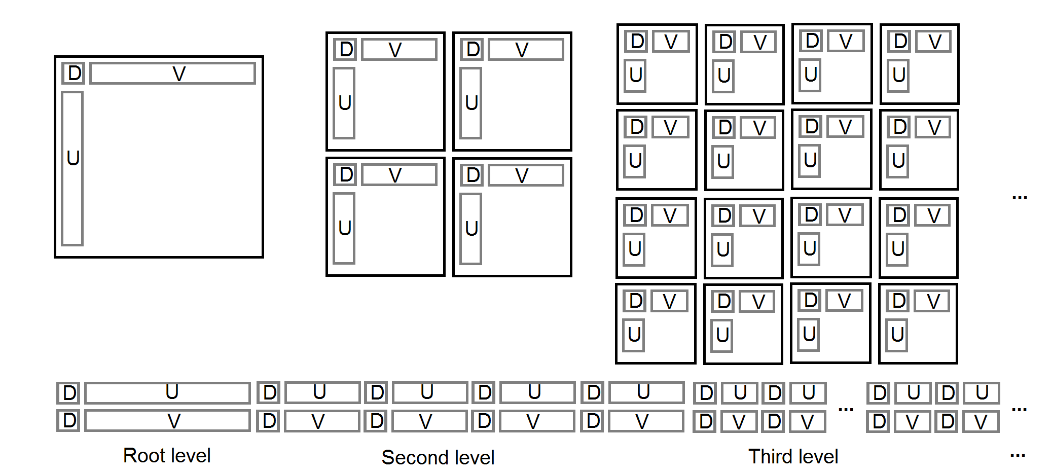
From the set $\mathcal{P}\subset\mathbb{R}^{d}$ of PDE-parameters, we can construct the neural network

where $\operatorname{DNN}(\mu)$ is the list of SVD decompositions for all $N_{B}$ blocks of different dimensions.

Unfortunately, training the neural networks $\mathbb{U}_{i}(\mu)$ and $\mathbb{V}_{i}(\mu)$ for different blocks, as functions of $\mu$ does not work. However, it is possible to train the singular values for different blocks as function of $\mu$, i.e.,

Knowing $\mathbb{D}_{i}(\mu)$ a priori for a given $\mu$ allows us to construct the structure of the hierarchical matrix, and call truncated SVD only for leaves of the matrix, which considerably speeds up the compression algorithm. An illustration of the architecture of the neural network used to learn singular values is depicted in Figure 7.

Given $\Omega=(0,1)^{2}\subset\mathbb{R}^{2}$ and $\beta=(1,0)$, we seek the solution of the advection-diffusion problem

where $\chi_{\{x=0\}}$ denotes the characteristic function over the the inflow boundary $x=0$.

The problem is driven by the inflow Dirichlet boundary condition and develops a boundary layer of width $\epsilon$ near the outflow $x=1$, as shown in Figure 8.

The weak form with a general Dirichlet boundary data $g\in H^{1\over 2}(\partial\Omega)$ will be to find $u^{\epsilon}\in H^{1}(\Omega)$ such that

To simplify the discussion, we approximate the solution as tensor products of one-dimensional B-splines basis functions $\{B_{i;p}(x)B_{j;p}(y)\}_{i,j}$ of uniform order $p$ in all directions. This discrete trial space $U_{h}^{p}\subset H^{1}(\Omega)$ will be split as $U_{h}^{p}=U_{h,0}^{p}+U^{p}_{h,\partial\Omega}$, where $U^{p}_{h,0}\subset H_{0}^{1}$ contains all the basis functions vanishing at $\partial\Omega$; and $U^{p}_{h,\partial\Omega}$ is the complementary subspace containing the basis functions associated with boundary nodes. Our discrete solution will be $u_{h}^{\epsilon}=u_{h,0}^{\epsilon}+u^{\epsilon}_{h,g}$, where $u^{\epsilon}_{h,0}\in U_{h,0}^{p}$ is unknown and $u^{\epsilon}_{h,g}\in U_{h,\partial\Omega}^{p}$ is directly obtained using the boundary data $g$.

We build the test space using a larger polynomial order $q>p$. That is, we use the tensor product of one-dimensional B-splines basis functions $\{B_{s;q}(x)B_{t;q}(y)\}_{s,t}$ of order $q$ and vanishing over $\partial\Omega$. This discrete test space will be denoted by $V^{q}_{h,0}\subset H_{0}^{1}(\Omega)$. The discrete residual minimization problem will be to find $u^{\epsilon}_{h,0}\in U_{h,0}^{p}$ and $r_{h}\in V_{h,0}^{q}$ such that

The reduced matrix system associated with (17) takes the form:

We train a neural network for the diagonal $\mathbb{D}(\epsilon)$ matrix of the SVD decomposition $[\mathbb{U}(\epsilon),\mathbb{D}(\epsilon),\mathbb{V}(\epsilon)]$ of the entire matrix $\mathbb{W}_{\epsilon}$ (see Figure 9), as well as $\mathbb{D}_{ij}(\epsilon)$ from the SVD decompositions $\{\mathbb{U}_{ij}(\epsilon),\mathbb{D}_{ij}(\epsilon),\mathbb{V}_{ij}(\epsilon)\}_{i=1,...,j^{2}}$ of sub-matrices obtained by $j\times j$ partitions of $\mathbb{W}_{\epsilon}$, for $j=2,4,8,16$. The white parts correspond to the boundary nodes, where we have enforced the boundary conditions. The convergence of the training procedures is presented in Figures 10.

In an online stage, for a given diffusion coefficient $\epsilon$, we perform the compression of the matrix $\mathbb{W}_{\epsilon}$ into the hierarchical matrix $\mathbb{H}_{\epsilon}$ using Algorithm 6, where the admissibility condition is now provided by the trained neural network. The compressed hierarchical matrices are illustrated in Figure 11.

Having the compressed matrix $\mathbb{H}_{\epsilon}$, we employ the GMRES algorithm [19] for solving the linear system (18). To avoid the computation with a dense $\mathbb{B}_{\epsilon}^{T}\mathbb{H}_{\epsilon}$ matrix, we note that the GMRES method involves computations of the residual $R=\mathbb{B}_{\epsilon}^{T}\mathbb{H}_{\epsilon}\,x-(L^{T}\mathbb{H}_{\epsilon})^{T}$ and the hierarchical matrix $\mathbb{H}_{\epsilon}$ enables matrix-vector multiplications of $\mathbb{H}_{\epsilon}\,x$ and $L^{T}\mathbb{H}_{\epsilon}$ in a quasi-linear computational cost.

In Table 1 we summarize the computational costs of our solver for two values of $\epsilon=\{0.1,0.000001\}$. The computational mesh was a tensor product of quadratic B-splines with 26 elements along $x$-axis and quadratic B-splines with 10 elements along $y$-axis. As we can read from the second and third columns, the DNN speeds up the compression process of the matrix of optimal test function’s coefficients around ten times. We employ the GMRES solver that computes the residual. The cost of multiplication of the $\mathbb{H}_{\epsilon}*x$ and the cost of multiplication of $\mathbb{A}*\mathbb{H}_{\epsilon}x$ is included in the fourth and fifth column in Table 1. The total cost of the GMRES with hierarchical matrices augmented by DNN compression is equal to compression cost of ${\mathbb{H}}_{\epsilon}$ with DNN plus number of iterations times the multiplication cost of ${\mathbb{H}}_{\epsilon}*x$ plus multiplication cost of ${\mathbb{A}}*{\mathbb{H}}_{\epsilon}x$. The total cost is presented in the last column of Table 1.

For comparison, we run the GMRES algorithm on the Galerkin method. The comparison is summarized in Table 2. The number of iterations, the cost per iteration, and the total cost are presented there. We can see that the cost of the stabilized solution is of the same order as the cost of the Galerkin solution. We compare here the costs of the correct solution obtained from the stable Petrov-Galerkin method with the cost of the incorrect solution from the unstable Galerkin method.

The numerical results are compared with the exact solutions in Figure 12 for inflow data $g=\sin(\pi y)$, and Figure 13 for inflow data $g=\sin(2\pi y)$.

Given $\Omega=(0,1)^{2}\subset\mathbb{R}^{2}$ and $\kappa\in[1,10]$, we seek the solution of the Hemholtz problem

with right-hand sides $f$ and $g$ such that the exact solution is $u(x,y)=\sin(\kappa\pi x)\sin(\kappa\pi y)$.

We employ $20\times 20$ finite elements mesh. The trial space is constructed from quadratic B-splines. The test space is obtained for trial, and quadraticfrom B-splines with $C^{0}$ separators (equivalent to Lagrange polynomials). The dependence of the coefficients of the optimal test functions on $\kappa$ for the Hemholtz problem has the affine structure described in Section 2.2, thus we can offline construct the function

where $\mathbb{W}(\kappa)$ is the matrix of the coefficients of the optimal test functions. We fix the trial and test spaces used for approximation of the solution and stabilization of the Petrov-Galerkin formulation. Next, we consider blocks of different size of matrix $\mathbb{W}(\kappa)$, and we train the SVD for these different blocks as function of $\kappa$, i.e.,

The convergence of the training procedure is presented in Figure 14. Knowing $\mathbb{D}_{i}(\kappa)$ a priori for a given $\kappa$ allows us to construct the structure of the hierarchical matrix, and we obtain the $\mathbb{U}_{i}(\kappa)$ and $\mathbb{V}_{i}(\kappa)$ from the neural networks.

Figure 15 depicts the exemplary resulting hierarchical matrices.

Table 3 summarizes the computational costs of our solver for two values of $\kappa=\{1,10\}$. The computational mesh was a tensor product of quadratic B-splines with 10 elements along $x$ and $y$ axes. The DNN allows obtaining the compression of the matrix of optimal test function’s coefficients for free. We employ the GMRES solver that computes the residual. The cost of multiplication of the $\mathbb{H}_{\kappa}*x$ and the cost of multiplication of $\mathbb{A}*\mathbb{H}_{\kappa}x$ is included in the fourth and fifth column in Table 3. The total cost of the GMRES with hierarchical matrices augmented by DNN compression is equal to the number of iterations times the multiplication cost of ${\mathbb{H}}_{\kappa}*x$ plus multiplication cost of ${\mathbb{A}}*{\mathbb{H}}_{\kappa}x$. The total cost is presented in the last column of Table 3.

We present in Table 4 the cost of the GMRES algorithm executed on the Galerkin method. We present the number of iterations, the cost per iteration, and the total cost. We can see that the cost of obtaining the stabilized solution is of the same order as the cost of the Galerkin method. We compare here the costs of the correct solution obtained from the Petrov-Galerkin method with the cost of the incorrect solution from the unstable Galerkin method.

The comparison of the solution obtained with the Petrov-Galerkin formulation with the optimal test functions generated by DNN and the exact solution is presented in Figure 16.

References

- [1] A. F. Agarap, Deep learning using rectified linear units (ReLu). arXiv preprint arXiv:1803.08375 (2018).
- [2] P. R. Amestoy and I. S. Duff, Multifrontal parallel distributed symmetric and unsymmetric solvers, Computer Methods in Applied Mechanics and Engineering, 184 (2000) 501-520.
- [3] P. R. Amestoy, I. S. Duff, J. Koster and J-Y L’Excellent, A fully asynchronous multifrontal solver using distributed dynamic scheduling, SIAM Journal on Matrix Analysis and Applications, 1(23) (2001) 15-41.
- [4] P. R. Amestoy, A. Guermouche, J-Y L’Excellent and S. Pralet, Hybrid scheduling for the parallel solution of linear systems, Computer Methods in Applied Mechanics and Engineering 2(32) (2001), 136–156.
- [5] V. M. Calo, Residual-based multiscale turbulence modeling: Finite volume simulations of bypass transition, Stanford University, Ph.D. Thesis (2005)
- [6] V. M. Calo, M. Łoś, Q. Deng, I. Muga, M. Paszyński, Isogeometric residual minimization method (iGRM) with direction splitting preconditioner for stationary advection-dominated diffusion problems, Computer Methods in Applied Mechanics and Engineering 373 (2021) 113214.
- [7] J. Chan, J. A.Evans, A minimal-residual finite element method for the convection-diffusion equations, ICES-REPORT 13-12 (2013)
- [8] J. Chan, J. A. Evans, W. Qiu. A dual Petrov–Galerkin fi- nite element method for the convection–diffusion equation. Computers & Mathematics with Applications 68(11) (2014) 1513–1529
- [9] A. Ern, J.-L. Guermond. Theory and practice of finite elements. Vol. 159. Springer, 2013
- [10] O.G. Ernst, M. J. Gander, Why it is Difficult to Solve Helmholtz Problems with Classical Iterative Methods. In: Graham, I., Hou, T., Lakkis, O., Scheichl, R. (eds.) Numerical Analysis of Multiscale Problems. Lecture Notes in Computational Science and Engineering, vol 83. Springer, Berlin, Heidelberg (2012)
- [11] W. Hackbush, Hierarchical Matrices: Algorithms and Analysis, Springer (2009)
- [12] R. A. Horn, C. R., Johnson, Matrix analysis. Cambridge university press. (1990)
- [13] T.J.R. Hughes, L.P. Franca, M. Mallet, A new finite element formulation for fluid dynamics: VI. Convergence analysis of the generalized SUPG formulation for linear time– dependent multidimensional advective–diffusive systems, Computer Methods in Applied Mechanics and Engineering, 6 (1987) 97–112.
- [14] D. P. Kingma, J. Ba. Adam: A method for stochastic optimization. arXiv preprint arXiv:1412.6980 (2014)
- [15] M. Łoś, I. Muga, J. Muñoz-Matute, M. Paszyński, Isogeometric Residual Minimization Method (iGRM) with direction splitting for non-stationary advection–diffusion problems, Computers & Mathematics with Applications, 79(2) (2020) 213-229.
- [16] M. Łoś, I. Muga, J. Muñoz-Matute, M. Paszyński, Isogeometric residual minimization (iGRM) for non-stationary Stokes and Navier–Stokes problems, Computers & Mathematics with Applications, 95(1) (2021) 200-214.
- [17] I. Muga, K. G. Van Der Zee. Discretization of Linear Prob- lems in Banach Spaces: Residual Minimization, Nonlinear Petrov–Galerkin, and Monotone Mixed Methods, SIAM Journal on Numerical Analysis 58(6) (2020), 3406–3426.
- [18] J. N. Reddy: An introduction to the finite element method, Mcgraw–Hill (2006)
- [19] Y. Saad, Iterative Methods for Sparse Linear Systems, Society for Industrial and Applied Mathematics; 2nd edition (2003)
- [20] R. Stevenson, J. Westerdiep, Minimal residual space-time discretizations of parabolic equations: Asymmetric spatial operators, Computers & Mathematics with Applications 101 (2021) 107-118