Towards Blind Watermarking: Combining Invertible and Non-invertible MechanismsCCS: Security and privacy Digital rights management

The research on digital watermark is first proposed in (Van Schyndel et al. 1994) in 1994, and it can be generally classified into two categories: traditional algorithms based on transform domain and a deep learning-based approach driven by data. Where the traditional watermarking methods include algorithms based on singular value decomposition (Soualmi et al. 2018; Mehta et al. 2016; Su et al. 2014), moment-based watermarking algorithms (Hu 1962; Hu et al. 2014) and transform domain watermarking algorithms (Alotaibi and Elrefaei 2019; Hamidi et al. 2018; Pakdaman et al. 2017). Accordingly, the deep learning-based watermarking model is first introduced by Hamidi et al. (Kandi et al. 2017) in 2017, whose method brings superior imperceptibility and robustness over traditional methods by employing an auto-encoder convolutional neural network(CNN). HiDDeN (Zhu et al. 2018) is the first to introduce the adversarial network to blind watermarking and also the first end-to-end method using neural networks. Subsequently, Ahmadi et al. (Ahmadi et al. 2020) propose a digital watermarking framework based on residual networks and achieved excellent robustness and imperceptibility. Liu et al. (Liu et al. 2019) propose the TSDL framework, which is composed of two-stage: noise-free end-to-end adversary training and noise-aware decoder-only training. This method is effective against black-box noise and can introduce non-differentiable noise attacks in the end-to-end network. Soon, Jia et al. (Jia et al. 2021) propose a novel Mini-Batch of Simulated and Real $Jpeg$ compression method to enhance robustness against $Jpeg$ compression, which performs excellent performance in various noises. In addition, there are works studying deep learning-based steganography and encryption (Sharma et al. 2019; Lu et al. 2021; Wengrowski and Dana 2019; Duan et al. 2019; Zhang et al. 2019) and a review of research on deep learning-based watermarking and steganography can be found (Zhang et al. 2021; Byrnes et al. 2021).

Invertible neural network is the first learning-based normalizing flow framework for modeling complex high-dimensional densities, proposed by Dinh et al. (Dinh et al. 2014) in 2014. To improve the efficiency and performance of image processing, Dinh et al. (Dinh et al. 2016) introduce convolutional layers in coupling models by modifying the additive coupling layers to both multiplication and addition, called real NVP. To further improve the coupling layer for density estimation and achieve better generation results, Kingma et al. (Kingma and Dhariwal 2018) propose a novel generative flow model based on the ActNorm layer and generalize channel-shuffle operations with invertible 1$\times$1 convolutions. Real NVP and 1$\times$1 convolutions are two frequently used structures in image tasks employing INN. Normalizing flow-based INN has become a popular choice in image generation tasks, and evolved with various similar deformations (Grathwohl et al. 2018; Kingma and Dhariwal 2018; Jacobsen et al. 2018; Behrmann et al. 2019; Chen et al. 2019). And there are also several approaches that incorporate INN with other methods, such as INN combined with self-attention (Ho et al. 2019) and INN constructed with masked convolutions (Song et al. 2019). Due to the flexibility and effectiveness of INN, it is also used for image super-resolution (Xiao et al. 2020; Lugmayr et al. 2020) and video super-resolution(Zhu et al. 2019). In addition, Ouderaa et al.(van der Ouderaa and Worrall 2019) applied INN to image-to-image translation, Wang et al.(Wang et al. 2020) applied INN in digital image compression, Ardizzone et al. (Ardizzone et al. 2019) introduce conditional INN for colorization, Liu et al. (Liu et al. 2021) propose an invertible denoising network, Xing et al. (Xing et al. 2021) propose an invertible image signal processing and Pumarola et al. (Pumarola et al. 2020) apply INN for image and 3D point cloud generation.

Fig. 5 shows the architecture of our proposed $CIN$, which is divided into the following parts: a Diffusion and Extraction Module (DEM), an Invertible Module (IM), a Fusion and split Module (FSM), a Non-invertible Attention-based Module (NIAM), and Noise-specific Selection Module (NSM). The embedding and extraction of CIN are defined as $f_{CIN}(\theta)$ and $f_{CIN}^{-1}(\theta)$.

The watermark $W_{m}$ is a binary sequence of length $L$ randomly sampled from $W_{m}\sim\{0,1\}^{L}$. Embedding the watermark into an RGB image $I_{m}$ with length and width of $H$ and $W$, respectively. Then the watermark and the image of the input model are $Wm\in\mathbb{R}^{B\times L}$ and $Im\in\mathbb{R}^{B\times C\times H\times W}$ respectively, where B and C refer to batchsize and channel number.

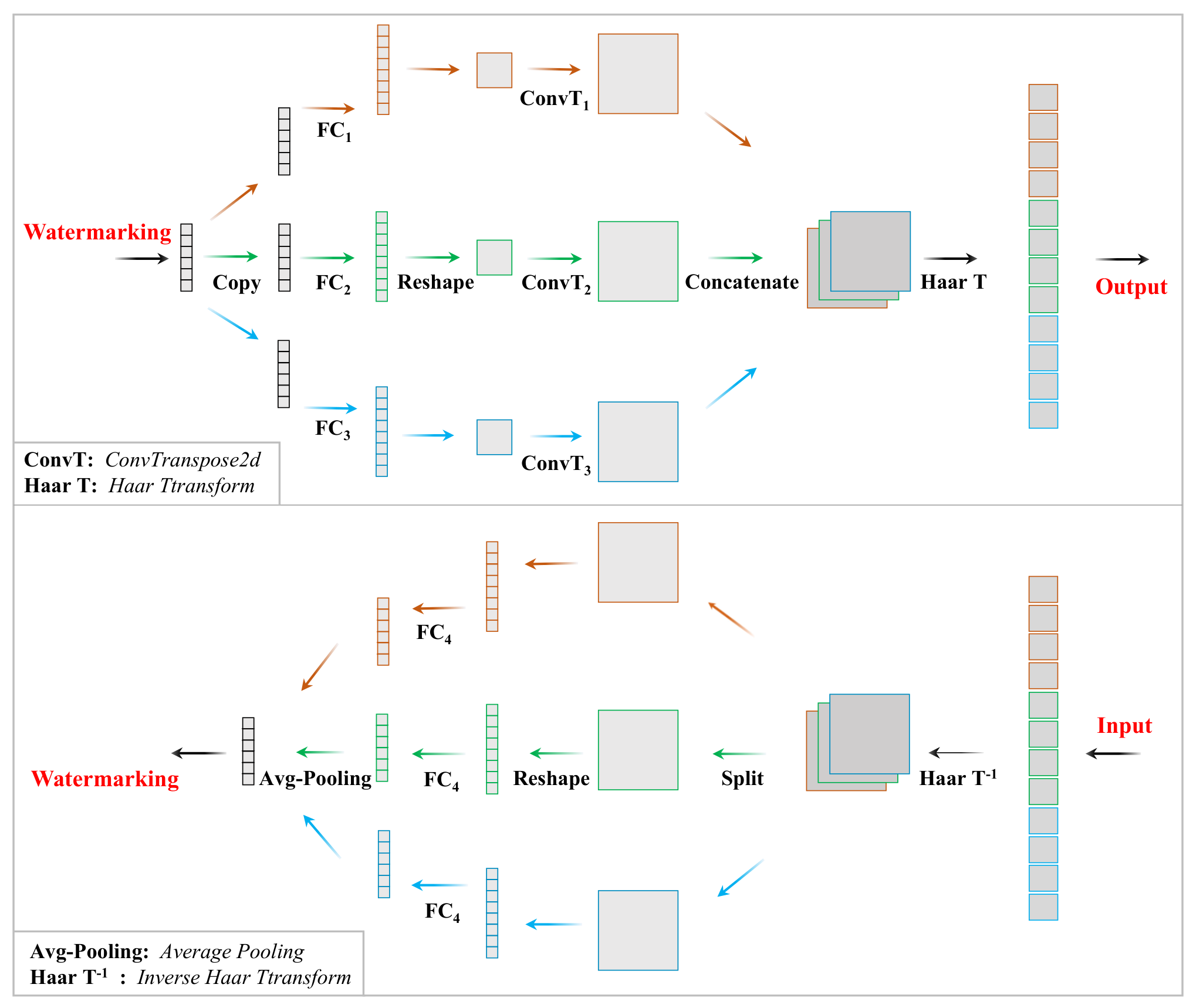
As shown in fig. 6, the top and bottom parts show the diffusion and extraction processes, respectively. In the diffusion processing, to align the watermark with the number of channels of the image, we first replicate the watermark $W_{m}$ in three copies. The different fully connected (FC) branches produce redundant watermarks of longer length, respectively. Subsequently, reshape and upsample to the same scale size as the cover image by two-dimensional transpose convolution (ConvT). After passing through the FC layer, the watermark length $\hat{L}$ is 256, the kernel size and stride of ConvT are both 2, and the block number is 3. Finally, the output of the three branches is concatenated and fed into the invertible module after the Haar transform. For forward embedding operations:

where ${\mathbf{O}}_{copy}\in 3\times\mathbb{R}^{B\times L}$, ${\mathbf{\Gamma}}_{fc}\in\mathbb{R}^{B\times\hat{L}}$, ${\mathbf{\Gamma}}_{convT}\in\mathbb{R}^{B\times 1\times H\times W}$, ${\mathbf{O}}_{cat}\in\mathbb{R}^{B\times 3\times H\times W}$ and ${\mathbf{\Gamma}}_{haar}\in\mathbb{R}^{B\times 12\times H/2\times W/2}$ refer to operations Copy, FC, ConvT, Concatenate and Haar Transform, respectively. And ${\mathbf{\Psi}}_{DEM}$ is the output tensor of Diffusion and Extract Module.

In the extraction process, the operation ${\mathbf{\Psi}^{-1}}_{DEM}$, which is the opposite of the embedding process, is taken for extraction. In contrast to Copy in the watermark embedding step, the final result is output by Average Pooling in the extraction process. The formula is as follows:

The coupling layer in the IM is an additive affine transformation, which was first proposed in NICE (Dinh et al. 2014). Recently, invertible architecture has been applied to information hiding with excellent representational capacity in works (Xiao et al. 2020; Guan et al. 2022; Lu et al. 2021), from which we were inspired. We use the watermark $W_{m}$ and the image $I_{m}$ as the two inputs of the invertible module, respectively. Our goal is to embed the $W_{m}$ into the $I_{m}$ with excellent imperceptibility and robustness.

The invertible module is shown in Fig. 4. The embedding and extraction correspond to the forward and backward of the bijection structure (Xiao et al. 2020), respectively. In the coupling layer of the $l^{th}$, $u_{wm}$ and $u_{im}$ denote the input watermark and image, respectively. The corresponding $u_{wm}^{l+1}$ and $u_{im}^{l+1}$ denote the output watermark and image after passing through the current coupling layer. The invertible module is formulated as:

where $\exp(\cdot)$ is exponential operator, $\phi(\cdot)$, $\rho(\cdot)$ and $\eta(\cdot)$ are arbitrary functions, $\odot$ is the Hadamard product. The corresponding backward propagation of the extraction process is formulated as:

The output ${\Psi}_{inv}\in\mathbb{R}^{B\times 24\times H/2\times W/2}$ of the invertible mudule (IM) can be split into two parts, ${\Psi}^{I}_{inv}(x;LR,HR)$ and ${\Psi}^{II}_{inv}(x;LR\_,HR\_)\in\mathbb{R}^{B\times 12\times H/2\times W/2}$. After Haar transform, the LR and HR represent the image’s low and high-frequency components. The left part of Fig. 7 is similar to the Channel Squeeze module of work (Cheng et al. 2021). The corresponding channels of the two outputs of the IM are averaged, which can be fused and squeezed to the size of the image. It is, however, difficult to trade off the watermark robustness with the imperceptibility. Therefore, we propose the fusion method as shown on the right in Fig. 7.

In the embedding process, we discard the image part of the IM output, keep only the mapped watermark part, and then add it to the image after scaling by the strength factor $S$ to obtain the final watermarked image. The formula is as follows:

where $S$ is the strength of the watermark. To restore the embedded watermark by invertible branch, the inputs are

where $\Gamma^{-1}_{haar}(\cdot)$ is inverse Haar transform.

The embedding and extraction of the watermark in invertible networks has a deterministic mapping relationship, which makes excellent results for watermark extraction accuracy in scenes without or with additive noise. However, when subjected to lossy compression or complex non-additive noise, since the forward and backward of the invertible network share the same set of parameters, the parameters of the decoder are updated along with the encoder, which limits the ability of the decoder to cope with complex noise. Therefore, an additional decoder is introduced in our framework to enhance the robustness of the invertible module against non-differentiable noise attacks, such as lossy compression noise. The non-invertible module uses SENet as the backbone to extract the watermark information $Wm_{2}$:

where $\mathbf{\Gamma}_{fc}(\cdot)$, $\mathbf{\Phi}_{SE}(\cdot)$, and ${\Gamma}_{conv}(\cdot)$ are FC, SENet and convolution layer, respectively.

Inspired by the article (Jia et al. 2021), we introduce differentiable and non-differentiable compression noise into the noise pool to push the NIAM robustness by encountering lossy compression. The network can update the parameters of both the IM and NIAM when introducing differentiable compression attack and only the NIAM for non-differentiable noise. For NSM, we employ a CNN-based noise discriminator to distinguish whether the attack is $Jpeg$ noise or not. If it is $Jpeg$, the selector exports $Wm_{2}$ extracted by NIAM; otherwise, return $Wm_{1}$ decoded by IM.

The robustness of the watermark is improved by introducing a noise layer in the architecture in (Luo et al. 2020; Liu et al. 2019; Zhu et al. 2018) et al.. To optimize the network parameters against the noise attack, it is generally necessary to use a differentiable noise layer trained jointly with the other basic module. In this work, the following 14 types of common noises:

$N_{pool}=\{Identity,JpegMask,RealJpeg,Crop,Cropout,Resize,\\ \hskip 30.00005ptGaussianBlur,SaltSalt\&Pepper,GaussianNoise,Dropout,\\ \hskip 30.00005ptBrightness,Contrast,Saturation,Hue\}$

where $JpegMask$ is the simulated differentiable $Jpeg$ noise (Jia et al. 2021). For resisting specific noise $RealJpeg$, we employ the following noise pool to train the model:

$N^{{cj}}_{pool}=\{JpegMask,RealJpeg\}$

To test the robustness of the model against simultaneous superimposed attacks of multiple noises, we use the following noise pool:

$N^{si}_{pool}=\{Identity,Cropout,Resize,Saturation,Hue,Dropout,\\ \hskip 50.00008ptGaussianBlur,SaltSalt\&Pepper,GaussianNoise\}$

For comparison with other works:

$N^{cp1}_{pool}=\{Identity,RealJpeg,Dropout,Cropout,Resize\}$

$N^{cp2}_{pool}=\{Identity,RealJpeg,Crop,Cropout,\\ \hskip 50.00008ptGaussianBlur,Dropout\}$

The loss functions constrain two parts: the watermarked image and the extracted watermark. Since the INN shares parameters for the embedding and extraction and has the same input and output dimensions, the loss constraint on the restored image in the noise-free version can also accelerate the convergence (Ardizzone et al. 2018).

Watermarked Image We employ $L_{2}$ loss to guide the watermarked image $WI_{m}$ to be visually alike to the reference image $I_{m}$:

Restored Watermark Calculate the $L_{2}$ distance for each pair of input watermark $W_{m}$ and the extracted watermark $RW_{m}$:

Restored Image When training the $CIN$ with $Identity$ noise layer, we employ $L_{2}$ distance to constrain the difference between the restored image $RI_{m}$ and the reference image $I_{m}$:

Total Loss To sum up, our $CIN$ is optimized by minimizing the compact loss $\mathcal{L}_{total}$, with the corresponding weight coefficients $\lambda_{WIm}$, $\lambda_{RWm}$ and $\lambda_{RIm}$:

The baseline model (denote as CIN*) contains only the invertible part. Using the method proposed in the article (Zhu et al. 2018) to concatenate each bit watermark after duplication with the image channels. And the channel squeezing method proposed in the article (Cheng et al. 2021) is used to output the watermarked image, as shown in the left part of Fig. 7. The specific architecture of CIN* is given in the Appendix. The results of the reference models are from either the published results or the open-source works and are partially quoted from the article (Zhang et al. 2020). Our experimental setup is consistent with the reference method.

To verify the robustness and imperceptibility of the proposed $CIN$, we utilize the real-world acquired COCO dataset (Lin et al. 2014) for training and evaluation. We also evaluate the transform performance of the model on the super-resolution dataset DIV2K dataset (Agustsson and Timofte 2017). For the COCO dataset, 10000 images are collected for training, and evaluation is performed on the other 5000 images. For the DIV2K dataset, we use 100 images from the validation set for evaluation. For each input image, there is a corresponding watermarking message which is randomly sampled from the binary distribution $W_{m}\sim\{0,1\}^{L}$.

To objectively evaluate the robustness and imperceptibility of our proposed watermarking framework, we apply a series of quantitative metrics. To validate the robustness, we evaluate the accuracy ($Acc$) between the extracted $RW_{m}$ and the embedded $W_{m}$. For each input image $I_{m}(x_{i})$, its corresponding watermark embedded and restored are $W_{m}(x_{i})$ and $RW_{m}(x_{i})$, respectively. Bit Error Ratio ($BER$) is also listed below, and the corresponding $Acc(\%)$ is $(1-BER)$.

For imperceptibility of watermarked images, we adopt the Peak Signal-to-Noise Ratio ($PSNR$) and Structural Similarity ($SSIM$) for evaluation.

where $MAX(\cdot)$ is the maximum pixel value of images, and $MSE(\cdot)$ represents the Mean Squared Error. Symbol $\sigma$, $\mu_{x}$ and $\sigma_{xy}$ represent the average, variances and covariance of images, respectively. $C1$ and $C2$ are two constants for preventing unstable results.

To keep a fair comparison, we adopt exactly the same settings with the reference methods. Images are resized to 128$\times$128 for all models, and the watermark length is 30 or 64. For our model, training with Nvidia 3080 graphics cards, the batch size is set to 32, and the Adam optimizer (Kingma and Ba 2014) with default hyperparameters is adopted. In the implementation, we train and evaluate the model under Specific Noise and Combined Noise, respectively. In the Specific Noise, all training and evaluations are performed only for one noise. In the Combined Noise, each mini-batch randomly samples a specific noise from $N_{pool}$, $N^{cp1}_{pool}$ or $N^{cp2}_{pool}$. In the evaluation stage, we utilize the trained model to test the performance of each noise in turn. Throughout the training phase, we first trained the model in the noise-free case, at which point the loss weights are set to $\lambda_{WIm}=1$, $\lambda_{RWm}=0.001$ and $\lambda_{RIm}=1$, respectively. Next, the model is trained to resist different noise. We load the trained noise-free model and subsequently set the loss weights to $\lambda_{WIm}=1$, $\lambda_{RWm}=0.01$ and $\lambda_{RIm}=0$, respectively. In training combined noise $N_{pool}$, $N^{cp1}_{pool}$ and $N^{cp2}_{pool}$, the loss weight are set to $\lambda_{WIm}=1$, $\lambda_{RWm}=1$ and $\lambda_{RIm}=0$, respectively. More experimental details can be found in the Appendix.

The results of our model $CIN$ against various noises are visualized in Fig. 8. Each column indicates the result against a specific noise. And we omit the results of noise $Identity$, $Cropoout$, and $Dropout$ since they appear almost identical to the input image. The first two rows are the input image $I_{m}$ and the output watermarked image $WI_{m}$, respectively. We can find that the image $WI_{m}$ and $I_{m}$ are almost indistinguishable visually, which indicates that our model has excellent imperceptibility. The third row is the noised image $I_{m}^{noised}$ attacked by the specific noise. The bottom row shows the magnified difference $|I_{m}^{noised}-WI_{m}|$ between the watermarked image $WI_{m}$ and the noised image $I_{m}^{noised}$, which indirectly indicates the intensity of the noise. In the Appendix, we present detailed noise parameters and experimental results against rotation, affine, and combinatorial attacks.

The detailed experimental performance corresponding to Fig. 8 is listed in Table 1. In the $Identity$ case, the $PSNR$ reaches $67.66dB$ with $BER$ less than $10^{-4}$, which demonstrates the high imperceptibility of our framework. The results are given for the two mechanisms of specific and combined noise. For specific noise, we list the $PSNR_{1}$ between $I_{m}$ and $WI_{m}$, the $PSNR_{2}$ between $WI_{m}$ and $I_{m}^{noised}$, the $Pretraining$ ($Pre$) accuracy tested on the $Identity$ model and the accuracy ($Acc$) tested on the specific noise model. The average $PSNR$ and $Acc$ with specific noise reach $54.76dB$ and $99.78\%$ respectively, which indicates that our framework has great potential against specific noise we have no test. For combined noise, we list the $Acc$ of the restored watermark $RWm$ and the $PSNR$ between $I_{m}^{noised}$ and $WI_{m}$. Moreover, the mean values of $PSNR$ and $Acc$ with the combined noises $N_{pool}$ reach $39.28dB$ and $99.64\%$, respectively.

As shown in Fig. 9, we visualize the watermark patterns that the model tends to embed for different noises. The watermarked pixel with $Identity$ is relatively concentrated in areas with texture information where watermarks can be easily embedded, while the region of the combined model and $Crop$ are more globally embedded to resist multiple noise and random cropping. $RealJpeg$ model is embedded in a way that can resist quantization loss.

In this work, we compare with several outstanding methods, such as HiDDeN (Zhu et al. 2018), DA (Luo et al. 2020), ABDH (Yu 2020), IGA (Zhang et al. 2020), TSDL (Liu et al. 2019), ReDMark (Ahmadi et al. 2020), and MBRS (Jia et al. 2021). To evaluate the performance of our model compared with other methods, we conducte experiments using noise $N^{cp1}_{pool}$ in Table 2. Our model not only has a higher $PSNR$ than other methods but also achieves the best results in terms of robustness.

In Table 3, all models are trained and evaluated with watermark length $L=30$. We find that our model can resist more kinds of noise ($N_{pool}$ has 12 types of noise) while achieving optimal robustness and a much higher $PSNR$ than other methods.

We conducte experiments with noise pool $N^{cp2}_{pool}$ in Table 4. At watermark length $L$=30, the PNSR is considerably higher than the reference method, and the $BER$ is lower. At $L$=64, our approach is significantly more robust to cropping than MBRS and has a slightly higher $PNSR$. Our method achieves excellent results in terms of robustness and imperceptibility compared to the SOTA MBRS (Jia et al. 2021).

In Fig. 10, the comparison experiments with the model MBRS show that our framework achieves higher $PSNR$ and $SSIM$ at lower $BER$. Meanwhile, in the experiments with higher $Jpeg$ compression strength, as shown in the left part for Q=10, our $BER$ is significantly lower than MBRS. In addition, as shown in the right part, our $SSIM$ is also noticeably higher than the reference at the strength factor of 1.4.

Through the ablation experiments in Table 5, we can find that when only the IM module (ICN*) is available, the $Acc$ against $RealJpeg$ is 77.49%, and the watermark intensity cannot be flexibly adjusted. After adding the DEM and FSM modules, the $Acc$ of the watermark improves by 7.2%, and the $PSNR$ improves by 2.38%. Finally, after employing NIAM and NSM modules, the model’s accuracy against $RealJpeg$ improves by 16.9%, and the $PSNR$ and the $Acc$ of resistance to multiple noises are also enhanced.