跳到论文正文
W Papers独立论文阅读器 arXiv:2212.12593 论文正文 计算阅读时间 · 0%
引用这篇论文根据当前论文元数据生成,正式投稿前建议核对。


License: CC BY 4.0
arXiv:2212.12593v2 [math.NA] 12 Apr 2023

Convexification Numerical Method for a Coefficient Inverse Problem for the Riemannian Radiative Transfer Equation Thanks: 2023.04.12

Michael V. Klibanov Email: mklibanv@uncc.edu Email: loc.nguyen@uncc.edu Thanks:  Department of Mathematics and Statistics, University of North Carolina at Charlotte, Charlotte, NC, 28223, USA (, )    Jingzhi Li Email: li.jz@sustech.edu.cn Thanks:  Department of Mathematics & National Center for Applied Mathematics Shenzhen & SUSTech International Center for Mathematics, Southern University of Science and Technology, Shenzhen 518055, P.˜R.˜China ()    Loc H. Nguyen 22footnotemark: 2    Vladimir G. Romanov Email: romanov@math.nsc.ru Thanks:  Sobolev Institute of Mathematics, Novosibirsk, 630090, Russian Federation ()    Zhipeng Yang Email: yangzp@sustech.edu.cn Thanks:  Department of Mathematics, Southern University of Science and Technology, Shenzhen 518055, P.˜R.˜China ()
Abstract

The first globally convergent numerical method for a Coefficient Inverse Problem (CIP) for the Riemannian Radiative Transfer Equation (RRTE) is constructed. This is a version of the so-called “convexification” method, which has been pursued by this research group for a number of years for some other CIPs for PDEs. Those PDEs are significantly different from the RRTE. The presence of the Carleman Weight Function (CWF) in the numerical scheme is the key element which insures the global convergence. Convergence analysis is presented along with the results of numerical experiments, which confirm the theory. RRTE governs the propagation of photons in the diffuse medium in the case when they propagate along geodesic lines between their collisions. Geodesic lines are generated by the spatially variable dielectric constant of the medium.

keywords
geodesic lines, Riemannian metric, Carleman estimate, coefficient inverse problem, global convergence, convexification, numerical studies
Funding.
The work of J. Li was partially supported by the NSF of China No. 11971221, Guangdong NSF Major Fund No. 2021ZDZX1001, the Shenzhen Sci-Tech Fund No. RCJC20200714114556020, JCYJ20200109115422828 and JCYJ20190809150413261. The work of L.H. Nguyen was partially supported by National Science Foundation grant DMS-2208159 and by funds provided by the Faculty Research Grant program at University of North Carolina at Charlotte, Fund No. 111272. The work by V.G. Romanov was performed within the state assignment of the Sobolev Institute of Mathematics of the Siberian Branch of the Russian Academy of Science, project number FWNF-2022-0009.
††runningheads: Convexification method for CIP for RRTE / M. V. Klibanov, J. Li, L. H. Nguyen, V. G. Romanov and Z. Yang
MSC
35R30, 65M32

1 Introduction

The conventional steady state radiative transfer equation (RTE) governs light propagation in the diffuse medium, such as, e.g. turbulent atmosphere and biological media [22]. Inverse problems for the RTE have applications in, e.g. problems of seeing through a turbulent atmosphere and in an early medical diagnostics. In the latter case the near infrared light with a relatively small energy of photons is used, see, e.g. [5]. However, it is assumed in the RTE that photons propagate along straight lines between their collisions. On the other hand, since the dielectric constants in heterogeneous media, such as, e.g. ones mentioned above, vary in space, then photons actually propagate along geodesic lines between their collisions. These lines are generated by the Riemannian metric εr​(𝐱)​|d​𝐱|.\sqrt{\varepsilon_{r}\left(\mathbf{x}\right)}\left|d\mathbf{x}\right|. Here and below 𝐱=(x,y,z)∈ℝ3\mathbf{x}=\left(x,y,z\right)\in\mathbb{R}^{3} and εr​(𝐱)\varepsilon_{r}\left(\mathbf{x}\right) is the spatially distributed dielectric constant, so that n⁡(𝐱)=εr​(𝐱)n\left(\mathbf{x}\right)=\sqrt{\varepsilon_{r}\left(\mathbf{x}\right)} is the refractive index. To take this into account, the so-called Riemannian Radiative Transfer Equation (RRTE) should be used.

This is the first publication, in which a globally convergent numerical method, the so-called convexification method, is constructed for a Coefficient Inverse Problem (CIP) for the steady state RRTE. In the past, numerical methods for inverse problems for the steady state RTE were mostly developed for the case of inverse source problems [13, 14, 47]. Inverse source problems are linear. On the other hand, CIPs are nonlinear. We refer to two recent publications of this research team [34, 35] for two versions of the convexification numerical method for a CIP for the RTE. The presence of the Riemannian aspect in the RRTE causes significant additional difficulties for the corresponding CIP, as compared with the case of the RTE in [34, 35]. The authors are unaware about other numerical methods for CIPs neither for the RTE nor for the RRTE.

Various uniqueness and stability results for inverse problems for both RTE and RRTE, including quite general forms of the latter equation, were published in the past. Since this paper is concerned only with a numerical method, then we refer now only to a limited number of such publications [3, 4, 5, 17, 27, 36, 38, 41].

The phenomena of ill-posedness and nonlinearity of CIPs are well known and cause serious challenges for their numerical solutions. Both a powerful and popular concept of numerical methods for CIPs is based on the minimization of appropriate least squares cost functionals, see, e.g. [1, 7, 6, 18, 19, 16, 21] and references cited therein. Since such a cost functional is typically non convex, then it usually suffers from the phenomenon of local minima and ravines, see, e.g. [46], i.e. the availability of a good first guess about the true solution is a necessary assumption of the convergence analysis of these numerical methods.

Remark 1.1. We call a numerical method for a CIP globally convergent if a theorem is proven, which claims that this method delivers at least one point in a sufficiently small neighborhood of the true solution without any advanced knowledge of this neighborhood. The size of that neighborhood should depend only on the level of noise in the data.

The key element of our numerical method is the presence of a Carleman Weight Function (CWF) in a certain weighted least squares cost functional. This presence ensures the global strict convexity of that functional. This is why we call our method “convexification”. The CWF is the function, which is involved as the weight function in the Carleman estimate for the corresponding PDE operator. Our convergence analysis ensures the global convergence of the gradient descent method of the minimization of that functional to the true solution of our CIP, as long as the level of the noise in the data tends to zero. The apparatus of the Riemannian geometry is also used here. Results of numerical experiments are presented, and they confirm our theory.

The convexification concept generates globally convergent numerical methods since these methods do not rely on good first guesses about the solutions. The convexification was originally proposed in purely theoretical works [32, 29]. Its active numerical studies have started in 2017 after the publication [2], which has removed some obstacles for numerical implementations. In this regard, we refer to, e.g. [26, 33, 34, 35] and references cited therein.

Another important new element of this paper is Theorem 1 (section 3), which claims existence, uniqueness and positivity of the solution of for the forward problem for the RRTE. An analog of this theorem for the non-Riemannian case was proven in [34]. The proof of Theorem 1 is constructive since it ends up with an analysis of a linear integral equation of the Volterra type. This equation is quite helpful in our numerical studies in section 6, since we solve it numerically to computationally simulate the data for the inverse problem. It is well known that such computational simulations form an important part of numerical studies of any inverse problem. The presence of the Riemannian aspect creates a significant additional difficulty in the proof of Theorem 1, as compared with the case of RTE in [34]. This difficulty is due to the necessity of working with the differential geometry, which, however, was not necessary to do in [34].

As to the apparatus of Carleman estimates, it was introduced in the field of CIPs in the publication [10], initially with the single goal of proofs of uniqueness theorems. Since then the idea of [10] was explored in many other publications, see, e.g. [8, 11, 12, 17, 23, 28, 30, 33, 38, 50] and references cited therein. The convexification principle represents an extension of the idea of [10] to the topic of globally convergent numerical methods for CIPs. Those numerical methods might be generalized and employed for important applications like, e.g. cloaking and quantum scattering studied in [40, 39].

We consider below only real valued functions. For the sake of definiteness, we work below in our theoretical derivations only with the 3d case. On the other hand, we present numerical results in the 2d case since the theory for the 2d case is completely similar with the one in the 3d case. In section 2 we pose both the forward and inverse problems for RRTE. In section 3 we formulate and prove the above mentioned Theorem 1. In section 4 we derive a version of the convexification method for our CIP. In section 5 we provide convergence analysis. Section 6 is devoted to numerical studies, which confirm our theory.

2 Statements of Forward and Inverse Problems

Let numbers A,a,b,d>0A,a,b,d>0, where

0<a<b.0<a<b. (2.1)

Define the rectangular prism Ω⊂ℝ3\Omega\subset\mathbb{R}^{3} and parts ∂1Ω,∂2Ω,∂3Ω\partial_{1}\Omega,\partial_{2}\Omega,\partial_{3}\Omega of its boundary ∂Ω,\partial\Omega, as well as the line Γd\Gamma_{d} where the external sources are:

Ω={𝐱:−A<x,y<A,a<z<b},∂1Ω={𝐱:−A<x,y<A,z=a}, ∂2Ω={𝐱:−A<x,y<A,z=b},∂3Ω={x=±A,y∈(−A.A),z∈(a,b)}∪∪{y=±A,x∈(−A,A),z∈(a,b)},Γd={𝐱α=(α,0,0):α∈[−d,d]}.\left.\begin{array}[]{c}\Omega=\{\mathbf{x}:-A<x,y<A,a<z<b\},\\ \partial_{1}\Omega=\left\{\mathbf{x}:-A<x,y<A,z=a\right\},\text{ }\partial_{2}\Omega=\left\{\mathbf{x}:-A<x,y<A,z=b\right\},\\ \partial_{3}\Omega=\left\{x=\pm A,y\in(-A.A),z\in\left(a,b\right)\right\}\cup\\ \cup\left\{y=\pm A,x\in(-A,A),z\in\left(a,b\right)\right\},\\ \Gamma_{d}=\{\mathbf{x}_{\alpha}=(\alpha,0,0):\alpha\in[-d,d]\}.\end{array}\right. (2.2)

Hence, Γd\Gamma_{d} is a part of the x−x-axis. By (2.1) and (2.2) Γd∩Ω¯=∅\Gamma_{d}\cap\overline{\Omega}=\varnothing.

Let the points of external sources 𝐱α∈Γd\mathbf{x}_{\alpha}\in\Gamma_{d}. Let ϵ>0\epsilon>0 be a sufficiently small number. To avoid dealing with singularities, we model the δ⁡(𝐱)−\delta\left(\mathbf{x}\right)-function as:

f⁡(𝐱)=Cϵ​{exp⁡(|𝐱|2ϵ2−|𝐱|2),|𝐱|<ϵ,0,|𝐱|≥ϵ,f\left(\mathbf{x}\right)=C_{\epsilon}\left\{\begin{array}[]{cc}\exp\left(\frac{\left|\mathbf{x}\right|^{2}}{\epsilon^{2}-\left|\mathbf{x}\right|^{2}}\right),&\left|\mathbf{x}\right|<\epsilon,\\ 0,&\left|\mathbf{x}\right|\geq\epsilon,\end{array}\right. (2.3)

where the constant CϵC_{\epsilon} is such that

Cϵ​∫|𝐱|<ϵexp⁡(|𝐱|2ϵ2−|𝐱|2)​𝑑𝐱=1.C_{\epsilon}\int_{\left|\mathbf{x}\right|<\epsilon}\exp\left(\frac{\left|\mathbf{x}\right|^{2}}{\epsilon^{2}-\left|\mathbf{x}\right|^{2}}\right)d\mathbf{x}=1. (2.4)

Hence, the function f⁡(𝐱−𝐱α)=f⁡(x−α,y,z)∈C∞​(ℝ3)f\left(\mathbf{x}-\mathbf{x}_{\alpha}\right)=f\left(x-\alpha,y,z\right)\in C^{\infty}\left(\mathbb{R}^{3}\right) plays the role of the source function for the point source {𝐱α}\left\{\mathbf{x}_{\alpha}\right\}. We choose ϵ\epsilon so small that

f⁡(𝐱−𝐱α)=0,∀𝐱∈Ω¯,∀𝐱α∈Γd.f\left(\mathbf{x}-\mathbf{x}_{\alpha}\right)=0,\quad\forall\mathbf{x}\in\overline{\Omega},\quad\forall\mathbf{x}_{\alpha}\in\Gamma_{d}. (2.5)

Let Γ⁡(𝐱,𝐱0)\Gamma(\mathbf{x},\mathbf{x}_{0}) be the geodesic line generated by the Riemannian metric εr​(𝐱)​|d​𝐱|\sqrt{\varepsilon_{r}\left(\mathbf{x}\right)}\left|d\mathbf{x}\right| and connecting the source 𝐱0∈ℝ3\mathbf{x}_{0}\in\mathbb{R}^{3} with an arbitrary point 𝐱∈ℝ3\mathbf{x}\in\mathbb{R}^{3},

Γ(𝐱,𝐱0)=argmin{∫γεr​(ξ​(t))​𝑑t, where ​γ​(t):[0,1]→ℝ3is a smooth map with γ(0)=𝐱0, γ(0)=𝐱.}\Gamma(\mathbf{x},\mathbf{x}_{0})=\text{argmin}\left\{\begin{array}[]{c}\int\limits_{\gamma}\sqrt{\varepsilon_{r}\left(\mathbf{\xi}\left(t\right)\right)}dt,\text{ where }\gamma\left(t\right):[0,1]\rightarrow\mathbb{R}^{3}\\ \text{is a smooth map with }\gamma\left(0\right)=\mathbf{x}_{0},\text{ }\gamma\left(0\right)=\mathbf{x}.\end{array}\right\} (2.6)

Here εr​(𝐱)\varepsilon_{r}\left(\mathbf{x}\right) is the spatially distributed dielectric constant of the medium, 1/εr​(𝐱)1/\sqrt{\varepsilon_{r}\left(\mathbf{x}\right)} is the dimensionless speed of light. We assume that the function εr​(𝐱)\varepsilon_{r}\left(\mathbf{x}\right) satisfies the following conditions:

εr​(𝐱)\displaystyle\varepsilon_{r}(\mathbf{x}) ∈C3​(ℝ3),\displaystyle\in C^{3}(\mathbb{R}^{3}), (2.7)
εr​(𝐱)\displaystyle\varepsilon_{r}(\mathbf{x}) =1,𝐱∈{𝐱∈ℝ3||x|≥A,|y|≥A}∪{𝐱∈ℝ3|z≤a},\displaystyle=1,\quad\mathbf{x}\in\{\mathbf{x}\in\mathbb{\ R}^{3}\big\rvert\ \rvert x\rvert\geq A,\rvert y\rvert\geq A\}\cup\{\mathbf{x}\in\mathbb{R}^{3}\big\rvert\ z\leq a\}, (2.8)
∂zεr​(𝐱)\displaystyle\partial_{z}\varepsilon_{r}(\mathbf{x}) ≥0,𝐱∈ℝ3.\displaystyle\geq 0,\quad\mathbf{x}\in\mathbb{R}^{3}. (2.9)

Let τ⁡(𝐱,𝐱0)\tau(\mathbf{x},\mathbf{x}_{0}) be the first time of arrival at the point 𝐱\mathbf{x} of light generated at the point 𝐱0.\mathbf{x}_{0}. Then [44, Chapter 3]

τ⁡(𝐱,𝐱0)=∫Γ⁡(𝐱,𝐱0)εr​(ξ​(σ))​𝑑σ,\tau(\mathbf{x},\mathbf{x}_{0})=\int\limits_{\Gamma(\mathbf{x},\mathbf{x}_{0})}\sqrt{\varepsilon_{r}\left(\mathbf{\xi}\left(\sigma\right)\right)}d\sigma, (2.10)

where d​σd\sigma is the element of the Euclidian length. For 𝐱≠𝐱0\mathbf{x}\neq\mathbf{x}_{0} the function τ⁡(𝐱,𝐱0)\tau(\mathbf{x},\mathbf{x}_{0}) is twice continuously differentiable with respect to 𝐱,𝐱0\mathbf{x},\mathbf{x}_{0} and is the solution of the eikonal equation [44, Chapter 3]

∣∇𝐱τ(𝐱,𝐱0)∣2=εr(𝐱), τ(𝐱,𝐱0)=O(∣𝐱−𝐱0∣),𝐱→𝐱0.\mid\nabla_{\mathbf{x}}\tau(\mathbf{x},\mathbf{x}_{0})\mid^{2}=\varepsilon_{r}(\mathbf{x}),\text{ }\tau(\mathbf{x},\mathbf{x}_{0})=O\left(\mid\mathbf{x}-\mathbf{x}_{0}\mid\right),\quad\mathbf{x}\rightarrow\mathbf{x}_{0}. (2.11)

We assume everywhere below that the geodesic lines are regular [44, Chapter 3]:

Regularity Assumption. Any two points 𝐱,𝐱0∈ℝ3\mathbf{x,x}_{0}\in\mathbb{R}^{3} can be connected by a single geodesic line Γ⁡(𝐱,𝐱0).\Gamma(\mathbf{x,x}_{0}).

A sufficient condition guaranteeing the regularity of geodesic lines can be found in [45]. Let μa​(𝐱)\mu_{a}\left(\mathbf{x}\right) and μs​(𝐱)\mu_{s}(\mathbf{x}) be the absorption and scattering coefficients of light respectively and let

μa​(𝐱),μs​(𝐱)≥0,μa​(𝐱),μs​(𝐱)∈C1​(ℝ3),μa(𝐱)=μs(𝐱)=0,𝐱∈ℝ3∖Ω,a⁡(𝐱)=μa​(𝐱)+μs​(𝐱).\left.\begin{array}[]{c}\mu_{a}\left(\mathbf{x}\right),\mu_{s}(\mathbf{x})\geq 0,\quad\mu_{a}\left(\mathbf{x}\right),\mu_{s}(\mathbf{x})\in C^{1}\left(\mathbb{R}^{3}\right),\\ \mu_{a}\left(\mathbf{x}\right)=\mu_{s}(\mathbf{x})=0,\quad\mathbf{x}\in\mathbb{R}^{3}\setminus\Omega,\\ a\left(\mathbf{x}\right)=\mu_{a}\left(\mathbf{x}\right)+\mu_{s}(\mathbf{x}).\end{array}\right. (2.12)

The function a⁡(𝐱)a\left(\mathbf{x}\right) is the attenuation coefficient. By (2.12)

a(𝐱)≥0,𝐱∈ℝ3, a(𝐱)∈C1(ℝ3),a(𝐱)=0,𝐱∈ℝ3∖Ω.a\left(\mathbf{x}\right)\geq 0,\ \mathbf{x}\in\mathbb{R}^{3},\text{ }a\left(\mathbf{x}\right)\in C^{1}\left(\mathbb{R}^{3}\right),\quad a\left(\mathbf{x}\right)=0,\ \mathbf{x}\in\mathbb{R}^{3}\setminus\Omega. (2.13)

Let A~=max⁡(A,d)\widetilde{A}=\max(A,d). Introduce three domains G,Ga+G,G_{a}^{+} and Ga−,G_{a}^{-},

G={𝐱:−A~<x,y<A~,z∈(0,b)},Ga+=G∪{z>a},Ga−=G∖Ga+.G=\left\{\mathbf{x}:-\widetilde{A}<x,y<\widetilde{A},z\in(0,b)\right\},G_{a}^{+}=G\cup\{z>a\},G_{a}^{-}=G\setminus G_{a}^{+}. (2.14)

Below we write sometimes u⁡(𝐱,α)u(\mathbf{x},\alpha) instead of u⁡(𝐱,𝐱α)u(\mathbf{x},\mathbf{x}_{\alpha}).

The Forward Problem. Find the solution u⁡(𝐱,α)∈C1​(G×[−d,d])u(\mathbf{x},\alpha)\in C^{1}\Big(G\times\left[-d,d\right]\Big) of the following problem:

(∇𝐱τ​(𝐱,𝐱α)/εr​(𝐱))⋅∇𝐱u​(𝐱,α)+a⁡(𝐱)​u​(𝐱,α)==μs(𝐱)∫ΓdK(𝐱,α,β)u(𝐱,β)dβ+f(𝐱−𝐱α), 𝐱∈G,𝐱α∈Γd,\left.\begin{array}[]{c}\left(\nabla_{\mathbf{x}}\tau(\mathbf{x},\mathbf{x}_{\alpha})/\sqrt{\varepsilon_{r}(\mathbf{x})}\right)\cdot\nabla_{\mathbf{x}}u(\mathbf{x},\alpha)+a(\mathbf{x})u(\mathbf{x},\alpha)=\\ =\mu_{s}(\mathbf{x})\int_{\Gamma_{d}}K(\mathbf{x},\alpha,\beta)u(\mathbf{\ x},\beta)d\beta+f(\mathbf{x}-\mathbf{x}_{\alpha}),\text{ }\mathbf{\ x}\in G,\mathbf{x}_{\alpha}\in\Gamma_{d},\end{array}\right. (2.15)
u⁡(𝐱α,𝐱α)=0​ for ​𝐱α∈Γd.u(\mathbf{x}_{\alpha},\mathbf{x}_{\alpha})=0\text{ for }\mathbf{x}_{\alpha}\in\Gamma_{d}. (2.16)

Definition 2.1. We call equation (2.15) the Riemannian Radiative Transfer Equation (RRTE).

In (2.15), (2.16) u⁡(𝐱,α)u(\mathbf{x},\alpha) denotes the steady-state radiance at the point 𝐱\mathbf{x} generated by the source function f⁡(𝐱−𝐱α)f\left(\mathbf{x}-\mathbf{x}_{\alpha}\right). The kernel K⁡(𝐱,α,β)K(\mathbf{x},\alpha,\beta) of the integral operator in (2.15) is called the “phase function” [22],

K(𝐱,α,β)≥0,𝐱∈Ω¯;α,β∈[−d,d],K⁡(𝐱,α,β)∈C1​(Ω¯×[−d,d]2).\left.\begin{array}[]{c}K(\mathbf{x},\alpha,\beta)\geq 0,\quad\mathbf{x}\in\overline{\Omega};\quad\alpha,\beta\in\left[-d,d\right],\\ K(\mathbf{x},\alpha,\beta)\in C^{1}\left(\overline{\Omega}\times\left[-d,d\right]^{2}\right).\end{array}\right. (2.17)

Coefficient Inverse Problem. Let the function u⁡(𝐱,α)u\left(\mathbf{x},\alpha\right) ∈C1​(Ω¯CLOSE\in C^{1}(\overline{\Omega} ×[−d,d])\times\left[-d,d\right]) be the solution of the Forward Problem. Assume that the coefficient a⁡(𝐱)a\left(\mathbf{x}\right) of equation (2.15) is unknown. Determine the function a⁡(𝐱)a\left(\mathbf{x}\right), assuming that the following function g⁡(𝐱,α)g\left(\mathbf{x},\alpha\right) is known:

g⁡(𝐱,α)=u⁡(𝐱,α),∀𝐱∈∂Ω​╲​∂1Ω,∀α∈(−d,d).g\left(\mathbf{x},\alpha\right)=u\left(\mathbf{x},\alpha\right),\quad\forall\mathbf{x}\in\partial\Omega\diagdown\partial_{1}\Omega,\quad\forall\alpha\in\left(-d,d\right). (2.18)

3 Existence and Uniqueness Theorem for the Forward Problem

Consider the unit tangent vector ν\nu to the geodesic line Γ⁡(𝐱,𝐱α)\Gamma(\mathbf{x},\mathbf{x}_{\alpha}) at the point 𝐱\mathbf{x} [44, Chapter 3]

ν=∇𝐱τ​(𝐱,𝐱α)/εr​(𝐱).\nu=\nabla_{\mathbf{x}}\tau\left(\mathbf{x},\mathbf{x}_{\alpha}\right)/\sqrt{\varepsilon_{r}\left(\mathbf{x}\right)}.

Hence, the directional derivative Dν​qD_{\nu}q of an appropriate function q⁡(𝐱,α)q(\mathbf{x},\alpha) in the direction of the vector ν\nu is

Dν​q=∇𝐱τ​(𝐱,𝐱α)εr​(𝐱)⋅∇𝐱q​(𝐱,α).D_{\nu}q=\frac{\nabla_{\mathbf{x}}\tau(\mathbf{x},\mathbf{x}_{\alpha})}{\sqrt{\varepsilon_{r}(\mathbf{x})}}\cdot\nabla_{\mathbf{x}}q(\mathbf{x},\alpha). (3.1)

Hence, if the function q⁡(𝐱,𝐱α)q(\mathbf{x},\mathbf{x}_{\alpha}) solves problem (3.2), then qq is given by formula (3.3), where

∇𝐱τ​(𝐱,𝐱α)εr​(𝐱)⋅∇𝐱q(𝐱,𝐱α)=a(𝐱),q(𝐱α,𝐱α)=0,\frac{\nabla_{\mathbf{x}}\tau(\mathbf{x},\mathbf{x}_{\alpha})}{\sqrt{\varepsilon_{r}(\mathbf{x})}}\cdot\nabla_{\mathbf{x}}q(\mathbf{x},\mathbf{\ \ x}_{\alpha})=a(\mathbf{x}),\quad q(\mathbf{x}_{\alpha},\mathbf{x}_{\alpha})=0, (3.2)
q⁡(𝐱,𝐱α)=∫Γ⁡(𝐱,𝐱α)a⁡(ξ⁡(σ))​𝑑σ.q(\mathbf{x},\mathbf{x}_{\alpha})=\int\limits_{\Gamma(\mathbf{x},\mathbf{x}_{\alpha})}a\left(\mathbf{\xi}(\sigma)\right)d\sigma. (3.3)

Let

p⁡(𝐱,𝐱α)=exp⁡(∫Γ⁡(𝐱,𝐱α)a⁡(ξ⁡(σ))​𝑑σ).p(\mathbf{x},\mathbf{x}_{\alpha})=\exp\left(\int\limits_{\Gamma(\mathbf{x},\mathbf{x}_{\alpha})}a\left(\mathbf{\xi}(\sigma)\right)d\sigma\right). (3.4)

Then (3.1)-(3.4) imply:

Dν​p=a⁡(𝐱)​p.D_{\nu}p=a\left(\mathbf{x}\right)p. (3.5)

Multiply both sides of equation (2.15) by pp and use (3.1)-(3.5). Note that by (2.5) and (2.12) p⁡(𝐱,𝐱α)​f​(𝐱−𝐱α)=f⁡(𝐱−𝐱α).p(\mathbf{x},\mathbf{x}_{\alpha})f(\mathbf{x}-\mathbf{x}_{\alpha})=f(\mathbf{\ \ x}-\mathbf{x}_{\alpha}). We obtain

p​Dν​u+a⁡(𝐱)​p​u=μs​(𝐱)​p​∫ΓdK⁡(𝐱,α,β)​u​(𝐱,β)​dβ+f⁡(𝐱−𝐱α),p​Dν​u+a⁡(𝐱)​p​u=Dν​(p​u)−a⁡(𝐱)​p​u+a⁡(𝐱)​p​u=Dν​(p​u),Dν​(p​u)=μs​(𝐱)​p​∫ΓdK⁡(𝐱,α,β)​u​(𝐱,β)​dβ+f⁡(𝐱−𝐱α).\left.\begin{array}[]{c}pD_{\nu}u+a\left(\mathbf{x}\right)pu=\mu_{s}(\mathbf{x})p\int\limits_{\Gamma_{d}}K(\mathbf{x},\alpha,\beta)u(\mathbf{x},\beta)d\beta+f(\mathbf{x}-\mathbf{x}_{\alpha}),\\ pD_{\nu}u+a\left(\mathbf{x}\right)pu=D_{\nu}\left(pu\right)-a\left(\mathbf{x}\right)pu+a\left(\mathbf{x}\right)pu=D_{\nu}\left(pu\right),\\ D_{\nu}\left(pu\right)=\mu_{s}(\mathbf{x})p\int\limits_{\Gamma_{d}}K(\mathbf{x},\alpha,\beta)u(\mathbf{x},\beta)d\beta+f(\mathbf{x}-\mathbf{x}_{\alpha}).\end{array}\right. (3.6)

Let the equation of the geodesic line Γ⁡(𝐱,𝐱α)\Gamma(\mathbf{x},\mathbf{x}_{\alpha}) be ξ=ξ⁡(σ,α)∈Γ⁡(𝐱,𝐱α)\mathbf{\xi=\xi}\left(\sigma,\alpha\right)\in\Gamma(\mathbf{x},\mathbf{x}_{\alpha}), where σ\sigma is the Euclidean length of the part Γξ​(𝐱,𝐱α)\Gamma_{\mathbf{\xi}}(\mathbf{x},\mathbf{x}_{\alpha}) of the curve Γ⁡(𝐱,𝐱α),\Gamma(\mathbf{x},\mathbf{x}_{\alpha}), which connects points ξ\mathbf{\ \ \xi} and 𝐱α\mathbf{x}_{\alpha}. Integrating the last line of (3.6) along the vector ν\nu and taking into account the initial condition (2.16), we obtain for 𝐱∈G,𝐱α∈Γd\mathbf{x}\in G,\mathbf{x}_{\alpha}\in\Gamma_{d}

u(𝐱,𝐱α)=u0(𝐱,𝐱α)+p−1(𝐱,𝐱α)××∫Γ⁡(𝐱,𝐱α)p⁡(ξ⁡(σ,α),𝐱α)​μs​(ξ⁡(σ,α))​(∫ΓdK⁡(ξ⁡(σ,α),α,β)​u​(ξ⁡(σ,α),β)​dβ)​dσ,u0​(𝐱,𝐱α)=p−1​(𝐱,𝐱α)​∫Γ⁡(𝐱,𝐱α)f⁡(ξ⁡(σ,α)−𝐱α)​dσ.\left.\begin{array}[]{c}u(\mathbf{x},\mathbf{x}_{\alpha})=u_{0}(\mathbf{x},\mathbf{x}_{\alpha})+p^{-1}(\mathbf{x},\mathbf{x}_{\alpha})\times\\ \times\int\limits_{\Gamma(\mathbf{x},\mathbf{x}_{\alpha})}p(\mathbf{\xi}(\sigma,\alpha),\mathbf{x}_{\alpha})\mu_{s}(\mathbf{\xi}(\sigma,\alpha))\left(\int\limits_{\Gamma_{d}}K(\mathbf{\xi}(\sigma,\alpha),\alpha,\beta)u(\mathbf{\xi}(\sigma,\alpha),\beta)d\beta\right)d\sigma,\\ u_{0}(\mathbf{x},\mathbf{x}_{\alpha})=p^{-1}(\mathbf{x},\mathbf{x}_{\alpha})\int\limits_{\Gamma\left(\mathbf{x},\mathbf{x}_{\alpha}\right)}f(\mathbf{\xi}(\sigma,\alpha)-\mathbf{x}_{\alpha})d\sigma.\end{array}\right. (3.7)

Thus, we conclude that the solution of the Forward Problem (2.15), (2.16) is equivalent to the solution of integral equation (3.7).

Theorem 1. Assume that conditions (2.12) and (2.17) hold. Then there exists unique solution u⁡(𝐱,α)∈C1​(G×[d,d])u(\mathbf{x},\alpha)\in C^{1}\Big(G\times\left[d,d\right]\Big) of problem ( 2.15), (2.16). Furthermore, the following inequality is valid:

u⁡(𝐱,α)≥m>0​ for ​(𝐱,α)∈(G¯a+×[−d,d]),\displaystyle u(\mathbf{x},\alpha)\geq m>0\text{ for }(\mathbf{x},\alpha)\in\left(\overline{G}_{a}^{+}\times[-d,d]\right), (3.8)
m=min(𝐱,α)∈(G¯a+×[−d,d])⁡u0​(𝐱,α),\displaystyle\hskip 28.45274ptm=\min_{(\mathbf{x},\alpha)\in\left(\overline{G}_{a}^{+}\times[-d,d]\right)}u_{0}(\mathbf{x},\alpha), (3.9)

where the domain Ga+G_{a}^{+} is defined in (2.14). Solution of problem (2.15), (2.16) is equivalent to the solution of equation (3.7).

Proof. The equivalency was proven above in this section. Let 𝐱∗\mathbf{x}^{\ast} be the intersection point of the geodesic line Γ⁡(𝐱,𝐱α)\Gamma(\mathbf{x},\mathbf{x}_{\alpha}) with plane {z=a}\left\{z=a\right\}. Note that by (2.1), (2.2) and (2.8) Γ⁡(𝐱∗,𝐱α)\Gamma(\mathbf{x}^{\ast},\mathbf{x}_{\alpha}) is an interval of a straight line. Since by (2.1), (2.12) and (2.14) μs​(𝐱)=0\mu_{s}(\mathbf{x})=0 for 𝐱∈Ga−\mathbf{x}\in G_{a}^{-}, then the first two lines of (3.7) can be rewritten as:

u⁡(𝐱,𝐱α)=u0​(𝐱,𝐱α)++p−1(𝐱,𝐱α)∫Γ⁡(𝐱,𝐱⋆)(∫ΓdK^(ξ(σ,α),α,β)u(ξ(σ,α),β)dβ)dσ,\left.\begin{array}[]{c}u(\mathbf{x},\mathbf{x}_{\alpha})=u_{0}(\mathbf{x},\mathbf{x}_{\alpha})+\\ +p^{-1}(\mathbf{x},\mathbf{x}_{\alpha})\int\limits_{\Gamma(\mathbf{x},\mathbf{x}^{\star})}\left(\int\limits_{\Gamma_{d}}\widehat{K}(\mathbf{\xi}(\sigma,\alpha),\alpha,\beta)u(\mathbf{\xi}(\sigma,\alpha),\beta)d\beta\right)d\sigma,\end{array}\right. (3.10)

where the function u0​(𝐱,𝐱α)u_{0}(\mathbf{x},\mathbf{x}_{\alpha}) is given in the third line of (3.7) and

K^​(𝐱,α,β)=p⁡(𝐱,𝐱α)​μs​(𝐱)​K​(𝐱,α,β).\widehat{K}(\mathbf{x},\alpha,\beta)=p(\mathbf{x},\mathbf{x}_{\alpha})\mu_{s}(\mathbf{x})K(\mathbf{x},\alpha,\beta). (3.11)

Consider now equations of the geodesic lines. Denote

q1=τx(𝐱,𝐱α), q2=τy(𝐱,𝐱α), q3=τz(𝐱,𝐱α).q_{1}=\tau_{x}(\mathbf{x},\mathbf{x}_{\alpha}),\text{ }q_{2}=\tau_{y}(\mathbf{x},\mathbf{x}_{\alpha}),\text{ }q_{3}=\tau_{z}(\mathbf{x},\mathbf{x}_{\alpha}). (3.12)

Then formulas (3.4) and (3.7) of [44, Chapter 3] imply that equations of geodesic lines are:

d​xd​s=q1εr,d​yd​s=q2εr, d​zd​s=q3εr, \frac{dx}{ds}=\frac{q_{1}}{\varepsilon_{r}},\frac{dy}{ds}=\frac{q_{2}}{\varepsilon_{r}},\text{ }\frac{dz}{ds}=\frac{q_{3}}{\varepsilon_{r}},\text{ } (3.13)
d​q1d​s=∂xεr2​εr, d​q2d​s=∂yεr2​εr, d​q3d​s=∂zεr2​εr,\frac{dq_{1}}{ds}=\frac{\partial_{x}\varepsilon_{r}}{2\varepsilon_{r}},\text{ }\frac{dq_{2}}{ds}=\frac{\partial_{y}\varepsilon_{r}}{2\varepsilon_{r}},\text{ }\frac{dq_{3}}{ds}=\frac{\partial_{z}\varepsilon_{r}}{2\varepsilon_{r}},

where d​s=εr​(𝐱​(σ))​d​σds=\sqrt{\varepsilon_{r}(\mathbf{x}(\sigma))}d\sigma is the element of the Riemannian length. In the integral (3.10),

𝐱⁡(σ,α)=(x⁡(σ,α),y⁡(σ,α),z⁡(σ,α))∈Ω.\mathbf{x}(\sigma,\alpha)=\left(x(\sigma,\alpha),y(\sigma,\alpha),z(\sigma,\alpha)\right)\in\Omega. (3.14)

It follows from (2.9) and [37, Lemma 5.1] that there exists a number c>0c>0 such that

τz​(𝐱,𝐱α)≥c.\tau_{z}\left(\mathbf{x},\mathbf{x}_{\alpha}\right)\geq c. (3.15)

Hence, a combination of equation (3.12) with the last equation in (3.13) implies:

∂sz⁡(s,α)>0​ and ​∂σz⁡(σ,α)>0.\partial_{s}z(s,\alpha)>0\text{ and \ }\partial_{\sigma}z(\sigma,\alpha)>0. (3.16)

Consider the equation of the geodesic line Γ⁡(𝐱,𝐱⋆)\Gamma(\mathbf{x},\mathbf{x}^{\star}) in the form:

ξ⁡(σ,α)=(ξ⁡(σ,α),η⁡(σ,α),ζ⁡(σ,α))\mathbf{\xi}(\sigma,\alpha)=(\xi(\sigma,\alpha),\eta(\sigma,\alpha),\zeta(\sigma,\alpha)) (3.17)

Change variables in (3.17) by replacing the variable σ\sigma with the variable ζ=ζ⁡(σ,α)\zeta=\zeta(\sigma,\alpha). Let σ=σ⁡(ζ,α)\sigma=\sigma(\zeta,\alpha) be the inverse function. Then the equation of the geodesic line Γ⁡(𝐱,𝐱⋆)\Gamma(\mathbf{x},\mathbf{x}^{\star}) can be rewritten as

ξ=ξ^​(ζ,α)=ξ⁡(σ⁡(ζ,α),α)=(ξ⁡(σ⁡(ζ,α),α),η⁡(σ⁡(ζ,α),α),ζ),ζ∈(a,z).\mathbf{\xi}=\widehat{\mathbf{\xi}}(\zeta,\alpha)=\mathbf{\xi}(\sigma(\zeta,\alpha),\alpha)=(\xi(\sigma(\zeta,\alpha),\alpha),\eta(\sigma(\zeta,\alpha),\alpha),\zeta),\quad\zeta\in(a,z).

By (3.14), (3.16) and (3.17) the inverse function σ=σ⁡(ζ,α)\sigma=\sigma(\zeta,\alpha) is monotonically increasing with respect to ζ\zeta along the geodesic line Γ⁡(x,x⋆)\Gamma(x,x^{\star}), i.e. ∂ζσ⁡(ζ,α)>0.\partial_{\zeta}\sigma\left(\zeta,\alpha\right)>0. Hence, we change variables in the integral of (3.10) as: σ⇔ζ=ζ⁡(σ,α)\sigma\Leftrightarrow\zeta=\zeta(\sigma,\alpha). Then equation (3.10) can be rewritten as:

u⁡(𝐱,𝐱α)=u0​(𝐱,𝐱α)+∫az(∫ΓdK~​(𝐱,ξ^​(ζ,α),α,β,ζ)​u​(ξ^​(ζ,α),β)​𝑑β)​𝑑ζ,u(\mathbf{x},\mathbf{x}_{\alpha})=u_{0}(\mathbf{x},\mathbf{x}_{\alpha})+\int\limits_{a}^{z}\left(\int\limits_{\Gamma_{d}}\widetilde{K}(\mathbf{x},\widehat{\mathbf{\xi}}(\zeta,\alpha),\alpha,\beta,\zeta)u(\widehat{\mathbf{\xi}}(\zeta,\alpha),\beta)d\beta\right)d\zeta, (3.18)

where 𝐱∈Ga+,𝐱α∈Γd\mathbf{x}\in G_{a}^{+},\mathbf{x}_{\alpha}\in\Gamma_{d} and by (3.11)

K~​(𝐱,ξ,α,β,ζ)=1p⁡(𝐱,𝐱α)​K^​(ξ,α,β)​∂ζσ⁡(ζ,α).\widetilde{K}(\mathbf{x},\mathbf{\xi},\alpha,\beta,\zeta)=\frac{1}{p(\mathbf{x},\mathbf{x}_{\alpha})}\widehat{K}(\mathbf{\xi},\alpha,\beta)\partial_{\zeta}\sigma(\zeta,\alpha). (3.19)

Since we have the integral

∫az(…)​𝑑ζ\int\limits_{a}^{z}\left(...\right)d\zeta

in equation (3.18), then this is the integral equation of the Volterra type. It follows from (2.7), (2.17), (3.4), (3.11)-(3.13) and (3.19) that the kernel of equation (3.18) is a non negative continuously differentiable function of its variables (𝐱,α,β,z)∈G¯a+\left(\mathbf{x},\alpha,\beta,z\right)\mathbf{\in}\overline{G}_{a}^{+} ×Γ¯d\times\overline{\Gamma}_{d} ×Γ¯d×[a,b]\times\overline{\Gamma}_{d}\times[a,b]. Hence, there exists a number K0>0K_{0}>0 such that in (3.18), (3.19)

0≤K~​(𝐱,ξ,α,β,ζ)≤K0<∞​ in (3.18).0\leq\widetilde{K}(\mathbf{x},\mathbf{\xi},\alpha,\beta,\zeta)\leq K_{0}<\infty\text{ in (\ref{2.37}).} (3.20)

Since equation (3.18) is of the Volterra type, then its solution can be obtained iteratively as:

un​(𝐱,𝐱α)=∫az∫ΓdK~​(𝐱,ξ^​(ζ,α),α,β,ζ)​un−1​(ξ^​(ζ,α),β)​dβ​dζ,u⁡(𝐱,𝐱α)=∑n=0∞un​(𝐱,𝐱α)​.\left.\begin{array}[]{c}u_{n}(\mathbf{x},\mathbf{x}_{\alpha})=\int\limits_{a}^{z}\int\limits_{\Gamma_{d}}\widetilde{K}(\mathbf{x},\widehat{\mathbf{\xi}}(\zeta,\alpha),\alpha,\beta,\zeta)u_{n-1}(\widehat{\mathbf{\xi}}(\zeta,\alpha),\beta)d\beta d\zeta,\\ u(\mathbf{x},\mathbf{x}_{\alpha})=\sum_{n=0}^{\infty}u_{n}(\mathbf{x},\mathbf{x}_{\alpha})\text{.}\end{array}\right. (3.21)

It follows from (2.3), (2.4), (3.9) and (3.18)-(3.21) that

m≤u(𝐱,𝐱α)≤[max(𝐱,α)∈(Ga+×[−d,d])u0(𝐱,𝐱α)]××∑n=0∞(2dK0(z−a))n/n!, 𝐱∈Ga+,\left.\begin{array}[]{c}m\leq u(\mathbf{x},\mathbf{x}_{\alpha})\leq\left[\max_{(\mathbf{x},\alpha)\in\left(G_{a}^{+}\times[-d,d]\right)\ }u_{0}\left(\mathbf{x},\mathbf{x}_{\alpha}\right)\right]\times\\ \times\mathop{\displaystyle\sum}\limits_{n=0}^{\infty}\left(2dK_{0}(z-a)\right)^{n}/n!,\text{ }\mathbf{x}\in G_{a}^{+},\end{array}\right. (3.22)

where numbers mm and K0K_{0} are defined in (3.9) and (3.20) respectively. Estimate (3.8) follows from (3.22). Obviously the series of first derivatives of terms of (3.21) with respect to any of variables x,y,z,αx,y,z,\alpha also converges absolutely. Hence the function u⁡(𝐱,𝐱α)u(\mathbf{x},\mathbf{x}_{\alpha}) in (3.21) belongs to C1​(G¯a+×Γ¯d).C^{1}\Big(\overline{G}_{a}^{+}\times\overline{\Gamma}_{d}\Big). We set

u⁡(𝐱,𝐱α)={the right hand side of (3.21) for ​(𝐱,𝐱α)∈Ga+×Γd,u0​(𝐱,𝐱α)​ for ​(𝐱,𝐱α)∈Ga−×Γd.u(\mathbf{x},\mathbf{x}_{\alpha})=\left\{\begin{array}[]{c}\text{the right hand side of (\ref{2.40}) for }(\mathbf{x},\mathbf{x}_{\alpha})\in G_{a}^{+}\times\Gamma_{d},\\ u_{0}(\mathbf{x},\mathbf{x}_{\alpha})\text{ for }(\mathbf{x},\mathbf{x}_{\alpha})\in G_{a}^{-}\times\Gamma_{d}.\end{array}\right.

Hence, the so defined function u⁡(𝐱,𝐱α)∈C1​(G¯×Γ¯d).u(\mathbf{x},\mathbf{x}_{\alpha})\in C^{1}\left(\overline{G}\times\overline{\Gamma}_{d}\right). Thus, we have proven the existence of the solution u⁡(𝐱,α)∈C1​(G¯×[d,d])u(\mathbf{x},\alpha)\in C^{1}\left(\overline{G}\times\left[d,d\right]\right) of the Forward Problem (2.15), (2.16) as well as estimate (3.8). To prove uniqueness, one should set in (3.18) u0​(𝐱,𝐱α)≡0u_{0}\left(\mathbf{x},\mathbf{x}_{\alpha}\right)\equiv 0 and then proceed in the classical way of the proof of the uniqueness of the Volterra integral equation of the second kind. □\square

Remark 3.1. It follows from (3.7) and Theorem 1 that one can solve Forward Problem via the solution of the linear integral equation in (3.7). This is how we solve the forward problem (2.15), (2.16) in the numerical section 6 to generate the data for the inverse problem.

4 Convexification Numerical Method for the Coefficient Inverse Problem

4.1 An integral differential equation without the unknown coefficient a⁡(𝐱)a\left(\mathbf{x}\right)

By (2.3)-(2.5) equation (2.15) can be rewritten as:

(∇𝐱τ​(𝐱,𝐱α)/εr​(𝐱))⋅∇𝐱u​(𝐱,α)+a⁡(𝐱)​u​(𝐱,α)==μs(𝐱)∫ΓdK(𝐱,α,β)u(𝐱,β)dβ, (𝐱,α)∈Ω×(−d,d).\left.\begin{array}[]{c}\left(\nabla_{\mathbf{x}}\tau(\mathbf{x},\mathbf{x}_{\alpha})/\sqrt{\varepsilon_{r}(\mathbf{x})}\right)\cdot\nabla_{\mathbf{x}}u(\mathbf{x},\alpha)+a(\mathbf{x})u(\mathbf{x},\alpha)=\\ =\mu_{s}(\mathbf{x})\int\limits_{\Gamma_{d}}K(\mathbf{x},\alpha,\beta)u(\mathbf{x},\beta)d\beta,\text{ }\left(\mathbf{x},\alpha\right)\in\Omega\times\left(-d,d\right).\end{array}\right. (4.1)

It follows from (3.8) that we can consider a new function v⁡(𝐱,α),v(\mathbf{x},\alpha),

v⁡(𝐱,α)=ln⁡u⁡(𝐱,α),(𝐱,α)∈Ω×(−d,d).v(\mathbf{x},\alpha)=\ln u(\mathbf{x},\alpha),\quad\left(\mathbf{x},\alpha\right)\in\Omega\times\left(-d,d\right). (4.2)

By (4.2) u⁡(𝐱,α)=ev⁡(𝐱,α).u(\mathbf{x},\alpha)=e^{v(\mathbf{x},\alpha)}. Substituting this in (4.1), we obtain for (𝐱,α)∈Ω×(−d,d):\left(\mathbf{x},\alpha\right)\in\Omega\times\left(-d,d\right):

(∇𝐱τ​(𝐱,𝐱α)/εr​(𝐱))⋅∇𝐱v​(𝐱,α)+a⁡(𝐱)=e−v⁡(𝐱,α)​μs​(𝐱)​∫ΓdK⁡(𝐱,α,β)​ev⁡(𝐱,β)​𝑑β.\left(\nabla_{\mathbf{x}}\tau(\mathbf{x},\mathbf{x}_{\alpha})/\sqrt{\varepsilon_{r}(\mathbf{x})}\right)\cdot\nabla_{\mathbf{x}}v(\mathbf{x},\alpha)+a(\mathbf{x})=e^{-v(\mathbf{x},\alpha)}\mu_{s}(\mathbf{x})\int\limits_{\Gamma_{d}}K(\mathbf{x},\alpha,\beta)e^{v(\mathbf{x},\beta)}d\beta. (4.3)

In particular, (4.3) implies that we can calculate the function a⁡(𝐱)a(\mathbf{x}) by the following formula:

a(𝐱)=−∫Γd(∇𝐱τ(𝐱,𝐱α)/εr​(𝐱))⋅∇𝐱v(𝐱,α)dα++∫Γd(e−v⁡(𝐱,α)μs(𝐱)∫ΓdK(𝐱,α,β)ev⁡(𝐱,β)dβ)dα.\left.\begin{array}[]{c}a(\mathbf{x})=-\mathop{\displaystyle\int}\limits_{\Gamma_{d}}\left(\nabla_{\mathbf{x}}\tau(\mathbf{x},\mathbf{x}_{\alpha})/\sqrt{\varepsilon_{r}(\mathbf{x})}\right)\cdot\nabla_{\mathbf{x}}v(\mathbf{x},\alpha)d\alpha+\\ +\mathop{\displaystyle\int}\limits_{\Gamma_{d}}\left(e^{-v(\mathbf{x},\alpha)}\mu_{s}(\mathbf{x})\int\limits_{\Gamma_{d}}K(\mathbf{x},\alpha,\beta)e^{v(\mathbf{x},\beta)}d\beta\right)d\alpha.\end{array}\right. (4.4)

Hence, we now focus on the problem of the reconstruction of the function v⁡(𝐱,α)v(\mathbf{x},\alpha) from the function g⁡(𝐱,α)g(\mathbf{x},\alpha) given in (2.18). We have

τz​(𝐱,α)εr​(𝐱)​vz​(𝐱,α)=∂∂z​(τzεr​v)−∂∂z​(τzεr)​v.\frac{\tau_{z}\left(\mathbf{x},\alpha\right)}{\sqrt{\varepsilon_{r}(\mathbf{x})}}v_{z}\left(\mathbf{x},\alpha\right)=\frac{\partial}{\partial z}\left(\frac{\tau_{z}}{\sqrt{\varepsilon_{r}}}v\right)-\frac{\partial}{\partial z}\left(\frac{\tau_{z}}{\sqrt{\varepsilon_{r}}}\right)v. (4.5)

Introduce a new function w⁡(𝐱,α)w\left(\mathbf{x},\alpha\right) and express v⁡(𝐱,α)v\left(\mathbf{x},\alpha\right) through v⁡(𝐱,α),v\left(\mathbf{x},\alpha\right),

w⁡(𝐱,α)=(τz​(𝐱,α)/εr​(𝐱))​v​(𝐱,α),v⁡(𝐱,α)=(εr​(𝐱)/τz​(𝐱,α)).\left.\begin{array}[]{c}w\left(\mathbf{x},\alpha\right)=\left(\tau_{z}\left(\mathbf{x},\alpha\right)/\sqrt{\varepsilon_{r}\left(\mathbf{x}\right)}\right)v\left(\mathbf{x},\alpha\right),\\ v\left(\mathbf{x},\alpha\right)=\left(\sqrt{\varepsilon_{r}\left(\mathbf{x}\right)}/\tau_{z}\left(\mathbf{x},\alpha\right)\right).\end{array}\right. (4.6)

It follows from (3.15) that the second line of formula (4.6) makes sense. Thus, (4.5) becomes

τzεr​vz=wz−[∂∂z​(τzεr)​εrτz]​w.\frac{\tau_{z}}{\sqrt{\varepsilon_{r}}}v_{z}=w_{z}-\left[\frac{\partial}{\partial z}\left(\frac{\tau_{z}}{\sqrt{\varepsilon_{r}}}\right)\frac{\sqrt{\varepsilon_{r}}}{\tau_{z}}\right]w. (4.7)

Using (4.6), transform other terms of the differential operator in (4.3),

τxεr​vx=τxεr​∂∂x​(εrτz​w)=τxτz​wx+[τxεr​∂∂x​(εrτz)]​w.\frac{\tau_{x}}{\sqrt{\varepsilon_{r}}}v_{x}=\frac{\tau_{x}}{\sqrt{\varepsilon_{r}}}\frac{\partial}{\partial x}\left(\frac{\sqrt{\varepsilon_{r}}}{\tau_{z}}w\right)=\frac{\tau_{x}}{\tau_{z}}w_{x}+\left[\frac{\tau_{x}}{\sqrt{\varepsilon_{r}}}\frac{\partial}{\partial x}\left(\frac{\sqrt{\varepsilon_{r}}}{\tau_{z}}\right)\right]w. (4.8)

And similarly for (τy/εr)​vy.\left(\tau_{y}/\sqrt{\varepsilon_{r}}\right)v_{y}. Hence, (4.3) becomes

wz+(τx​wx+τy​wy)/τz++[(τx/εr)​∂x(εr/τz)+(τy/εr)​∂y(εr/τz)−(εr/τz)​∂z(τz/εr)]​w−−exp(−wεr/τz)(𝐱,α)μs(𝐱)∫ΓdK(𝐱,α,β)exp(wεr/τz)(𝐱,β)dβ==−a(𝐱), (𝐱,α)∈Ω×(−d,d).\left.\begin{array}[]{c}w_{z}+\left(\tau_{x}w_{x}+\tau_{y}w_{y}\right)/\tau_{z}+\\ +\left[\left(\tau_{x}/\sqrt{\varepsilon_{r}}\right)\partial_{x}\left(\sqrt{\varepsilon_{r}}/\tau_{z}\right)+\left(\tau_{y}/\sqrt{\varepsilon_{r}}\right)\partial_{y}\left(\sqrt{\varepsilon_{r}}/\tau_{z}\right)-\left(\sqrt{\varepsilon_{r}}/\tau_{z}\right)\partial_{z}\left(\tau_{z}/\sqrt{\varepsilon_{r}}\right)\right]w-\\ -\exp\left(-w\sqrt{\varepsilon_{r}}/\tau_{z}\right)(\mathbf{x},\alpha)\mu_{s}(\mathbf{x})\int\limits_{\Gamma_{d}}K(\mathbf{x},\alpha,\beta)\exp\left(w\sqrt{\varepsilon_{r}}/\tau_{z}\right)(\mathbf{x},\beta)d\beta=\\ =-a\left(\mathbf{x}\right),\text{ }\left(\mathbf{x},\alpha\right)\in\Omega\times\left(-d,d\right).\end{array}\right. (4.9)

Differentiate both sides of (4.9) with respect to α\alpha and use ∂αa⁡(𝐱)≡0\partial_{\alpha}a(\mathbf{x})\equiv 0. We obtain for (𝐱,α)∈Ω×(−d,d):\left(\mathbf{x},\alpha\right)\in\Omega\times\left(-d,d\right):

∂αwz+∂α((τx​wx+τy​wy)/τz)++∂α{[(τx/εr)∂x(εr/τz)+(τy/εr)∂y(εr/τz)]w}−−∂α[(εr/τz)∂z(τz/εr)w]−−∂α[exp(−wεr/τz)(𝐱,α)μs(𝐱)∫ΓdK(𝐱,α,β)exp(wεr/τz)(𝐱,β)dβ]=0.\left.\begin{array}[]{c}\partial_{\alpha}w_{z}+\partial_{\alpha}\left(\left(\tau_{x}w_{x}+\tau_{y}w_{y}\right)/\tau_{z}\right)+\\ +\partial_{\alpha}\left\{\left[\left(\tau_{x}/\sqrt{\varepsilon_{r}}\right)\partial_{x}\left(\sqrt{\varepsilon_{r}}/\tau_{z}\right)+\left(\tau_{y}/\sqrt{\varepsilon_{r}}\right)\partial_{y}\left(\sqrt{\varepsilon_{r}}/\tau_{z}\right)\right]w\right\}-\\ -\partial_{\alpha}\left[\left(\sqrt{\varepsilon_{r}}/\tau_{z}\right)\partial_{z}\left(\tau_{z}/\sqrt{\varepsilon_{r}}\right)w\right]-\\ -\partial_{\alpha}\left[\exp\left(-w\sqrt{\varepsilon_{r}}/\tau_{z}\right)(\mathbf{x},\alpha)\mu_{s}(\mathbf{x})\int\limits_{\Gamma_{d}}K(\mathbf{x},\alpha,\beta)\exp\left(w\sqrt{\varepsilon_{r}}/\tau_{z}\right)(\mathbf{x},\beta)d\beta\right]=0.\end{array}\right. (4.10)

The Dirichlet boundary condition for the function w⁡(𝐱,α)w(\mathbf{x},\alpha) is:

w⁡(𝐱,α)=τz​(𝐱,α)εr​(𝐱)​ln⁡g1​(𝐱,α),(𝐱,α)∈∂Ω×(−d,d),\displaystyle w(\mathbf{x},\alpha)=\frac{\tau_{z}(\mathbf{x},\alpha)}{\sqrt{\varepsilon_{r}\left(\mathbf{x}\right)}}\ln g_{1}(\mathbf{x},\alpha),\quad(\mathbf{x},\alpha)\in\partial\Omega\times(-d,d), (4.11)
g1​(𝐱,α)={g⁡(𝐱,α),𝐱∈∂Ω╲∂1Ω,α∈(−d,d),u0​(𝐱,α),𝐱∈∂1Ω,α∈(−d,d).\displaystyle\hskip 0.0ptg_{1}(\mathbf{x},\alpha)=\left\{\begin{array}[]{ll}g(\mathbf{x},\alpha),&\mathbf{x}\in\partial\Omega\diagdown\partial_{1}\Omega,\quad\alpha\in(-d,d),\\ u_{0}(\mathbf{x},\alpha),&\mathbf{x}\in\partial_{1}\Omega,\quad\alpha\in(-d,d).\end{array}\right.

Thus, we develop below a numerical method to obtain an approximate solution w⁡(𝐱,α)w(\mathbf{x},\alpha) of problem (4.10)-(4.1).

4.2 A special orthonormal basis in L2​(−d,d)L_{2}(-d,d)

First, we introduce a special orthonormal basis in L2​(−d,d),L_{2}(-d,d), which was first discovered in [31], also, see [33, section 6.2.3]. Consider a linearly independent set of functions {αn​eα}n=0∞⊂L2​(−d,d)\{\alpha^{n}e^{\alpha}\}_{n=0}^{\infty}\subset L_{2}(-d,d), which is complete in L2​(−d,d)L_{2}(-d,d). The Gram-Schmidt orthonormalization procedure being applied to this set, results in the orthonormal basis {Ψn​(α)}n=0∞\{\Psi_{n}\left(\alpha\right)\}_{n=0}^{\infty} in L2​(−d,d)L_{2}(-d,d). The Gram-Schmidt procedure is unstable when it is applied to an infinite number of functions. However, we have not seen an instability when applying it to a relatively small number of functions for n∈[0,12].n\in\left[0,12\right]. The same was observed in a number of previous publications of this research group, see, e.g. [26, 34], [33, Chapters 7,10,12].

Let [,]\left[,\right] be the scalar product in L2​(−d,d)L_{2}(-d,d). Denote bs,k=[Qs′,Qk].b_{s,k}=\left[Q_{s}^{\prime},Q_{k}\right]. Then [31], [33, section 6.2.3]

bs,k={1,s=k,0,s>k.b_{s,k}=\left\{\begin{array}[]{c}1,s=k,\\ 0,s>k.\end{array}\right. (4.14)

Consider the N×NN\times N matrix BN=(bs,k)(s,k)=(0,0)(N−1,N−1)B_{N}=\left(b_{s,k}\right)_{\left(s,k\right)=\left(0,0\right)}^{\left(N-1,N-1\right)}. Then (4.14) implies that detBN=1,\det B_{N}=1, which means that this matrix is invertible. In fact, the existence of the matrix BN−1B_{N}^{-1} for each N≥1N\geq 1 is the key property why the basis {Qn​(α)}n=0∞\{Q_{n}\left(\alpha\right)\}_{n=0}^{\infty} was originally constructed in [31]. Indeed, consider, for example either the basis of standard orthonormal polynomials or the basis of trigonometric functions. In each of these, the first function is an identical constant, which means that the first raw of an analog of the matrix BNB_{N} is zero.

4.3 A boundary value problem for a system of nonlinear PDEs

We assume that the functions w⁡(𝐱,α)w(\mathbf{x},\alpha), wα​(𝐱,α)w_{\alpha}(\mathbf{x},\alpha) can be represented as truncated Fourier-like series

w⁡(𝐱,α)=∑n=0N−1wn​(𝐱)​Qn​(α),wα​(𝐱,α)=∑n=0N−1wn​(𝐱)​Qn′​(α)w(\mathbf{x},\alpha)=\sum\limits_{n=0}^{N-1}w_{n}(\mathbf{x})Q_{n}(\alpha),\quad w_{\alpha}(\mathbf{x},\alpha)=\sum\limits_{n=0}^{N-1}w_{n}(\mathbf{\ \ x})Q_{n}^{\prime}(\alpha) (4.15)

with unknown coefficients {wn​(𝐱)}n=0N−1.\left\{w_{n}(\mathbf{x})\right\}_{n=0}^{N-1}. Thus, we focus below on the computation of the N−N-D vector function

V⁡(𝐱)=(w0,w1,⋯,wN−1)T​(𝐱).V(\mathbf{x})=\left(w_{0},w_{1},\cdots,w_{N-1}\right)^{T}(\mathbf{x}). (4.16)

Remarks 4.1:

  1. 1.

    The representations (4.15) mean that this is a version of the Galerkin method. However, unlike classical well-posed forward problems for PDEs, where Galerkin method is used and its convergence at N→∞N\rightarrow\infty is usually proven, we cannot prove convergence of our inversion numerical procedure described below for N→∞N\rightarrow\infty. This is basically because of the ill-posed nature of our CIP. Thus, we actually work below within the framework of an approximate mathematical model. Then, however, the question can be raised whether this model really works numerically. The answer is positive, and this answer is obtained computationally in section 6. We observe that very similar truncated series were used in some other above cited works on the convexification, such as, e.g. [26, 34], [33, Chapters 7,10], and all of them have demonstrated good numerical performances. Likewise, truncated Fourier series were used in works of other authors about CIPs, such as, e.g. [20, 24, 25, 42] and also without proofs of convergence of inversion procedures at N→∞.N\rightarrow\infty. Those proofs were not provided for the same reason as the one here: the ill-posed nature of CIPs.

  2. 2.

    Finally, we refer to subsection 3.4 of [34] for more arguments in support of those of item 1. In particular, these arguments include the well known fact that the Huygens-Fresnel theory of the diffraction in optics is not yet rigorously derived from the Maxwell’s equations, see, e.g. a classic textbook [9, pages 412, 413]. Philosophically, this fact is similar with the discussion of item 1.

Substitute (4.15) in (4.10). Next, sequentially multiply the obtained equation by Qn​(α)Q_{n}(\alpha), n=0,…,N−1n=0,...,N-1 and integrate with respect to α∈(−d,d).\alpha\in(-d,d). We obtain the following system of coupled quasilinear integral differential equations

BN​Vz​(𝐱)+A1​(𝐱)​Vx​(𝐱)+A2​(𝐱)​Vy​(𝐱)+F⁡(V⁡(𝐱),𝐱)=0,𝐱∈Ω,B_{N}V_{z}(\mathbf{x})+A_{1}(\mathbf{x})V_{x}(\mathbf{x})+A_{2}(\mathbf{x})V_{y}(\mathbf{x})+F\left(V(\mathbf{x}),\mathbf{x}\right)=0,\quad\mathbf{\ \ x}\in\Omega, (4.17)

where A1​(𝐱)A_{1}(\mathbf{x}) and A2​(𝐱)A_{2}(\mathbf{x}) are N×NN\times N matrices and F⁡(V⁡(𝐱),𝐱)F\left(V(\mathbf{x}),\mathbf{x}\right) is a certain vector function, which depends nonlinearly on V⁡(𝐱).V(\mathbf{x}). Explicit formulas for A1​(𝐱)A_{1}(\mathbf{x}), A2​(𝐱)A_{2}(\mathbf{x}) and F⁡(V⁡(𝐱),𝐱)F\left(V(\mathbf{x}),\mathbf{x}\right) can be easily written. However, we do not present them here for brevity. In addition, the boundary condition for the vector function V⁡(𝐱)V(\mathbf{x}) is:

V⁡(𝐱)∣∂Ω=P⁡(𝐱)=(p0,p1,⋯,pN−1)T​(𝐱),\displaystyle\hskip 28.45274ptV\left(\mathbf{x}\right)\mid_{\partial\Omega}=P(\mathbf{x})=\left(p_{0},p_{1},\cdots,p_{N-1}\right)^{T}(\mathbf{x}), (4.18)
pn(𝐱)=∫−dd[τz​(𝐱,α)εr​(𝐱)ln[g1(𝐱,α)]]Qn(α)dα,n=0,1,⋯,N−1.\displaystyle p_{n}(\mathbf{x})=\int\limits_{-d}^{d}\left[\frac{\tau_{z}(\mathbf{x},\alpha)}{\sqrt{\varepsilon_{r}\left(\mathbf{x}\right)}}\ln\left[g_{1}(\mathbf{x},\alpha)\right]\right]Q_{n}(\alpha)d\alpha,\quad n=0,1,\cdots,N-1. (4.19)

Thus, we now have to solve the boundary value problem (4.17)-(4.19).

To numerically calculate the derivatives of ∇𝐱τ​(𝐱,α)\nabla_{\mathbf{x}}\tau(\mathbf{x},\alpha) with respect to α\alpha, we represent ∇𝐱τ​(𝐱,α)\nabla_{\mathbf{x}}\tau(\mathbf{x},\alpha) via the truncated Fourier series with respect to the above basis {Qn​(α)}n=0N−1\left\{Q_{n}(\alpha)\right\}_{n=0}^{N-1} as:

∇𝐱τ​(𝐱,α)=∑n=0N−1(∇𝐱τ)n​(𝐱)​Qn​(α).\nabla_{\mathbf{x}}\tau(\mathbf{x},\alpha)=\sum\limits_{n=0}^{N-1}\left(\nabla_{\mathbf{x}}\tau\right)_{n}(\mathbf{x})Q_{n}(\alpha). (4.20)

Then we use explicit formulas for functions Qn​(α)Q_{n}(\alpha) to get

∂α(∇𝐱τ)=∑n=0N−1(∇𝐱τ)s​(𝐱)​Qn′​(α).\partial_{\alpha}\left(\nabla_{\mathbf{x}}\tau\right)=\sum\limits_{n=0}^{N-1}\left(\nabla_{\mathbf{x}}\tau\right)_{s}(\mathbf{x})Q_{n}^{\prime}(\alpha). (4.21)

Then equations (4.20) and (4.21) are used in (4.17)-(4.19). Thus, it follows from (4.10) and (4.15)-(4.21) that

{A1​(𝐱),A2​(𝐱)∈CN2​(Ω¯), and the vector functionF(V(𝐱),𝐱) is continuously differentiablewith respect to its arguments for ​𝐱∈Ω¯.\left\{\begin{array}[]{c}A_{1}(\mathbf{x}),A_{2}(\mathbf{x})\in C_{N^{2}}\left(\overline{\Omega}\right),\text{ and the vector function}\\ F\left(V\left(\mathbf{x}\right),\mathbf{x}\right)\text{ is continuously differentiable}\\ \text{with respect to its arguments for }\mathbf{x}\in\overline{\Omega}.\end{array}\right. (4.22)

Here and below for any integer k≥2k\geq 2 and for any Banach space BB we denote Bk=BkB_{k}=B^{k} with the norm ‖f‖Bk2=‖f1‖B2+…+‖fk‖B2,\left\|f\right\|_{B_{k}}^{2}=\left\|f_{1}\right\|_{B}^{2}+...+\left\|f_{k}\right\|_{B}^{2}, ∀f=(f1,…,fk)T∈Bk.\forall f=\left(f_{1},...,f_{k}\right)^{T}\in B_{k}.

4.4 Minimization problem

Let R>0R>0 be an arbitrary number and the vector function P⁡(x)P\left(x\right) be the boundary condition in (4.18). Define the set S⁡(R,P)⊂HN1​(Ω)S\left(R,P\right)\subset H_{N}^{1}\left(\Omega\right) as:

S(R,P)={V∈HN1(Ω):V(𝐱)∣∂Ω=P(𝐱),‖W‖HN1​(Ω)<R}.S\left(R,P\right)=\left\{V\in H_{N}^{1}\left(\Omega\right):V(\mathbf{x})\mid_{\partial\Omega}=P(\mathbf{x}),\left\|W\right\|_{H_{N}^{1}\left(\Omega\right)}<R\right\}. (4.23)

To solve problem (4.17)-(4.19), we solve the following minimization problem:

Minimization Problem 1. Let λ≥1\lambda\geq 1 be a parameter. Minimize the following weighted cost functional Jλ​(V)J_{\lambda}\left(V\right) on the set S⁡(R,P)¯:\overline{S\left(R,P\right)}:

Jλ​(V)=‖(BN​Vz+A1​(𝐱)​Vx​(𝐱)+A2​(𝐱)​Vy​(𝐱)+F⁡(V⁡(𝐱),𝐱))​eλ​z‖LN2​(Ω)2.\left.J_{\lambda}\left(V\right)=\left\|\left(B_{N}V_{z}+A_{1}(\mathbf{x})V_{x}(\mathbf{x})+A_{2}(\mathbf{x})V_{y}(\mathbf{x})+F\left(V(\mathbf{x}),\mathbf{x}\right)\right)e^{\lambda z}\right\|_{L_{N}^{2}\left(\Omega\right)}^{2}.\right. (4.24)

5 Convergence Analysis

We carry out the convergence analysis for a modified Minimization Problem 1. To obtain this modification, we rewrite the differential operator in functional (4.24) via finite differences with respect to the variables x,yx,y while leaving the conventional derivative with respect to zz. We call this “partial finite differences”.

5.1 Partial finite differences

Let m>1m>1 be an integer. Let A>0A>0 be the number in (2.2). Consider two partitions of the interval (−A,A)\left(-A,A\right),

−A=x0<x1<⋯<xm=A,xj+1−xj=h,j=0,⋯,m−1,−A=y0<y1<⋯<ym=A,yj+1−yj=h,j=0,⋯,m−1.\left.\begin{array}[]{c}-A=x_{0}<x_{1}<\cdots<x_{m}=A,\quad x_{j+1}-x_{j}=h,\quad j=0,\cdots,m-1,\\ -A=y_{0}<y_{1}<\cdots<y_{m}=A,\quad y_{j+1}-y_{j}=h,\quad j=0,\cdots,m-1.\end{array}\right. (5.1)

We assume that

h≥h0=c​o​n​s​t.>0.h\geq h_{0}=const.>0. (5.2)

Define the semidiscrete subset Ωh\Omega^{h} of the domain Ω\Omega as:

Ω1h={(xi,yj)}i,j=0m,\displaystyle\hskip 85.35826pt\Omega_{1}^{h}=\left\{\left(x_{i},y_{j}\right)\right\}_{i,j=0}^{m}, (5.3)
Ωh=Ω1h×(a,b)={(xi,yj):(xi,yj)∈Ω1h,z∈(a,b)}.\displaystyle\Omega^{h}=\Omega_{1}^{h}\times\left(a,b\right)=\left\{(x_{i},y_{j}):(x_{i},y_{j})\in\Omega_{1}^{h},z\in(a,b)\right\}. (5.4)

Below points (xi,yj,z)∈Ωh(x_{i},y_{j},z)\in\Omega^{h} are denoted as 𝐱h\mathbf{x}^{h}. By (2.2), (5.3) and (5.4) the boundary ∂Ωh\partial\Omega^{h} of the domain Ωh\Omega^{h} is:

∂Ωh=∂1Ωh∪∂2Ωh∪∂3Ωh,\displaystyle\hskip 42.67912pt\partial\Omega^{h}=\partial_{1}\Omega^{h}\cup\partial_{2}\Omega^{h}\cup\partial_{3}\Omega^{h},
∂1Ωh=Ω1h×{z=a},∂2Ωh=Ω1h×{z=b},\displaystyle\hskip 5.69046pt\partial_{1}\Omega^{h}=\Omega_{1}^{h}\times\left\{z=a\right\},\ \partial_{2}\Omega^{h}=\Omega_{1}^{h}\times\left\{z=b\right\},
∂3Ωh={(x0,yj,z),(xm,yj,z):z∈(a,b)}.\displaystyle\partial_{3}\Omega^{h}=\left\{\left(x_{0},y_{j},z\right),\left(x_{m},y_{j},z\right):z\in(a,b)\right\}.

Let the vector function Y⁡(𝐱)∈CN1​(Ω¯)Y(\mathbf{x})\in C_{N}^{1}(\overline{\Omega}). Denote

Yh​(𝐱h)=Y⁡(xi,yj,z),𝐱h=(xi,yj,z)∈Ωh.Y^{h}(\mathbf{x}^{h})=Y(x_{i},y_{j},z),\quad\mathbf{x}^{h}=(x_{i},y_{j},z)\in\Omega^{h}.

Thus, Yh​(𝐱h)Y^{h}(\mathbf{x}^{h}) is an N−DN-D vector function of discrete variables (xi,yj)∈Ω1h(x_{i},y_{j})\in\Omega_{1}^{h} and continuous variable z∈(a,b)z\in(a,b). Note that by (5.1) the boundary terms at ∂3Ωh\partial_{3}\Omega^{h} of this vector function, which correspond to Y⁡(𝐱)∣∂3ΩhY(\mathbf{x})\mid_{\partial_{3}\Omega^{h}}, are:

{Y⁡(x0,yj,z)}∪{Y⁡(xm,yj,z)}∪{Y⁡(xi,y0,z)}∪{Y⁡(xi,ym,z)},i,j=0,⋯,m.\left\{Y(x_{0},y_{j},z)\right\}\cup\left\{Y(x_{m},y_{j},z)\right\}\cup\left\{Y(x_{i},y_{0},z)\right\}\cup\left\{Y(x_{i},y_{m},z)\right\},i,j=0,\cdots,m.

For two vector functions Y(1)​(𝐱)=(Y0(1)​(𝐱),⋯,YN−1(1)​(𝐱))TY^{\left(1\right)}(\mathbf{x})=\left(Y_{0}^{\left(1\right)}(\mathbf{x}),\cdots,Y_{N-1}^{\left(1\right)}(\mathbf{x})\right)^{T} and Y(2)​(𝐱)=(Y0(2)​(𝐱)CLOSEY^{\left(2\right)}(\mathbf{x})=(Y_{0}^{\left(2\right)}(\mathbf{x}), ⋯\cdots, OPENYN−1(2)​(𝐱))TY_{N-1}^{\left(2\right)}(\mathbf{x}))^{T} their scalar product Y(1)​(𝐱)⋅Y(2)​(𝐱)Y^{\left(1\right)}(\mathbf{x})\cdot Y^{\left(2\right)}(\mathbf{x}) is defined as the scalar product in ℝN,\mathbb{R}^{N}, and (Y⁡(𝐱))2=Y⁡(𝐱)⋅Y⁡(𝐱)\left(Y(\mathbf{x})\right)^{2}=Y(\mathbf{x})\cdot Y(\mathbf{x}). Respectively,

Y(1)​h​(𝐱h)⋅Y(2)​h​(𝐱h)==∑n=0N−1∑(i,j)=(1,1)(i,j)=(m−1,m−1)Yn(1)​h​(xi,yj,z)​Yn(2)​h​(xi,yj,z),(Yh(𝐱h))2=Yh(𝐱h)⋅Yh(𝐱h), |Yh(𝐱h)|=Yh​(𝐱h)⋅Yh​(𝐱h).\left.\begin{array}[]{c}Y^{\left(1\right)h}(\mathbf{x}^{h})\cdot Y^{\left(2\right)h}(\mathbf{x}^{h})=\\ =\sum\limits_{n=0}^{N-1}\sum\limits_{\left(i,j\right)=\left(1,1\right)}^{\left(i,j\right)=\left(m-1,m-1\right)}Y_{n}^{\left(1\right)h}(x_{i},y_{j},z)Y_{n}^{\left(2\right)h}(x_{i},y_{j},z),\\ \left(Y^{h}(\mathbf{x}^{h})\right)^{2}=Y^{h}(\mathbf{x}^{h})\cdot Y^{h}(\mathbf{x}^{h}),\text{ }\left|Y^{h}(\mathbf{x}^{h})\right|=\sqrt{Y^{h}(\mathbf{x}^{h})\cdot Y^{h}(\mathbf{x}^{h})}.\end{array}\right. (5.5)

We will use formulas (5.5) everywhere below without further mentioning. We exclude here boundary terms with i,j=0i,j=0 and i,j=mi,j=m since we work below with finite difference derivatives as defined in the next paragraph.

We define finite difference derivatives of the semidiscrete N−N-D vector function Yh​(𝐱h)Y^{h}(\mathbf{x}^{h}) with respect to x,yx,y only at interior points of the domain Ωh\Omega^{h} with i,j=1,…,m−1i,j=1,...,m-1,

∂xYh​(xi,yj,z)=Yh​(xi,yj,z)x=(Yh​(xi+1,yj,z)−Yh​(xi−1,yj,z))/(2​h),∂xYh​(xi,yj,z)=Yh​(xi,yj,z)x=(Yh​(xi+1,yj,z)−Yh​(xi−1,yj,z))/(2​h),∂yYh​(xi,yj,z)=Yh​(xi,yj,z)y=(Yh​(xi,yj+1,z)−Yh​(xi,yj−1,z))/(2​h),Yxh(𝐱h)={Yh(xi,yj,z)x}i,j=1m−1, Yyh(𝐱h)={Yh(xi,yj,z)y}i,j=1m−1.\left.\begin{array}[]{c}\partial_{x}Y^{h}\left(x_{i},y_{j},z\right)=Y^{h}\left(x_{i},y_{j},z\right)_{x}=\left(Y^{h}\left(x_{i+1},y_{j},z\right)-Y^{h}\left(x_{i-1},y_{j},z\right)\right)/\left(2h\right),\\ \partial_{x}Y^{h}\left(x_{i},y_{j},z\right)=Y^{h}\left(x_{i},y_{j},z\right)_{x}=\left(Y^{h}\left(x_{i+1},y_{j},z\right)-Y^{h}\left(x_{i-1},y_{j},z\right)\right)/\left(2h\right),\\ \partial_{y}Y^{h}\left(x_{i},y_{j},z\right)=Y^{h}\left(x_{i},y_{j},z\right)_{y}=\left(Y^{h}\left(x_{i},y_{j+1},z\right)-Y^{h}\left(x_{i},y_{j-1},z\right)\right)/\left(2h\right),\\ Y_{x}^{h}\left(\mathbf{x}^{h}\right)=\left\{Y^{h}\left(x_{i},y_{j},z\right)_{x}\right\}_{i,j=1}^{m-1},\text{ }Y_{y}^{h}\left(\mathbf{x}^{h}\right)=\left\{Y^{h}\left(x_{i},y_{j},z\right)_{y}\right\}_{i,j=1}^{m-1}.\end{array}\right. (5.6)

We need semidiscrete analogs of spaces CN2​(Ω¯),HN1​(Ω),LN2​(Ω)C_{N^{2}}\left(\overline{\Omega}\right),H_{N}^{1}\left(\Omega\right),L_{N}^{2}\left(\Omega\right). All three are defined using the same principle. Hence, we provide here only two definitions: for the space HN1,h​(Ωh)H_{N}^{1,h}\left(\Omega^{h}\right) and its subspace HN,01,h​(Ωh)H_{N,0}^{1,h}\left(\Omega^{h}\right). Others are similar. We introduce the space HN1,h​(Ωh)H_{N}^{1,h}\left(\Omega^{h}\right) as:

HN1,h​(Ωh)=={Yh​(𝐱h):‖Yh​(𝐱h)‖HN1,h​(Ωh)2=∑i,j=1m−1∫ab(Yh​(xi,yj,z))2​dz++∑i,j=1m−1∫ab(Yxh(xi,yj,z))2dz+∑i,j=1m−1∫ab(Yyh(xi,yj,z))2dz++∑i,j=1m−1∫ab(Yzh(xi,yj,z))2dz<∞},\begin{split}&\hskip 113.81102ptH_{N}^{1,h}\left(\Omega^{h}\right)=\\ &=\left\{\begin{array}[]{c}Y^{h}(\mathbf{x}^{h}):\left\|Y^{h}(\mathbf{x}^{h})\right\|_{H_{N}^{1,h}\left(\Omega^{h}\right)}^{2}=\sum\limits_{i,j=1}^{m-1}\int\limits_{a}^{b}\left(Y^{h}\left(x_{i},y_{j},z\right)\right)^{2}dz+\\ +\sum\limits_{i,j=1}^{m-1}\int\limits_{a}^{b}\left(Y_{x}^{h}\left(x_{i},y_{j},z\right)\right)^{2}dz+\sum\limits_{i,j=1}^{m-1}\int\limits_{a}^{b}\left(Y_{y}^{h}\left(x_{i},y_{j},z\right)\right)^{2}dz+\\ +\sum\limits_{i,j=1}^{m-1}\int\limits_{a}^{b}\left(Y_{z}^{h}\left(x_{i},y_{j},z\right)\right)^{2}dz<\infty\end{array}\right\},\end{split} (5.7)
HN,01,h​(Ωh)={Yh​(𝐱h)∈HN1,h​(Ωh):Yh​(𝐱h)∣∂Ωh=0}.H_{N,0}^{1,h}\left(\Omega^{h}\right)=\left\{Y^{h}(\mathbf{x}^{h})\in H_{N}^{1,h}\left(\Omega^{h}\right):Y^{h}(\mathbf{x}^{h})\mid_{\partial\Omega^{h}}=0\right\}. (5.8)

By embedding theorem HN1,h​(Ωh)⊂CNh​(Ω¯h)H_{N}^{1,h}\left(\Omega^{h}\right)\subset C_{N}^{h}\left(\overline{\Omega}^{h}\right) and

‖Yh​(𝐱h)‖CNh​(Ω¯h)≤C​‖Yh​(𝐱h)‖HN1,h​(Ωh),∀Yh∈HN1,h​(Ωh),\left\|Y^{h}(\mathbf{x}^{h})\right\|_{C_{N}^{h}\left(\overline{\Omega}^{h}\right)}\leq C\left\|Y^{h}(\mathbf{x}^{h})\right\|_{H_{N}^{1,h}\left(\Omega^{h}\right)},\forall Y^{h}\in H_{N}^{1,h}\left(\Omega^{h}\right), (5.9)

where the number C=C⁡(h0,A,Ω)>0C=C\left(h_{0},A,\Omega\right)>0 depends only on listed parameters, where h0h_{0} is defined in (5.2). Also, it follows from (5.2), (5.6) that

‖Yxh(𝐱h‖L2,h​(Ωh),‖Yyh(𝐱h‖L2,h​(Ωh)≤C‖Yh(𝐱h‖L2,h​(Ωh).\left\|Y_{x}^{h}(\mathbf{x}^{h}\right\|_{L^{2,h}\left(\Omega^{h}\right)},\left\|Y_{y}^{h}(\mathbf{x}^{h}\right\|_{L^{2,h}\left(\Omega^{h}\right)}\leq C\left\|Y^{h}(\mathbf{x}^{h}\right\|_{L^{2,h}\left(\Omega^{h}\right)}. (5.10)

The following formulas are semidiscrete analogs of (4.15):

wh(𝐱h,α)=∑n=0N−1wnh(𝐱h)Qn(α), ∂αwh(𝐱h,α)=∑n=0N−1wnh(𝐱h)Qn′(α).w^{h}(\mathbf{x}^{h}\mathbf{,}\alpha)=\sum\limits_{n=0}^{N-1}w_{n}^{h}(\mathbf{x}^{h})Q_{n}(\alpha),\text{ }\partial_{\alpha}w^{h}(\mathbf{x}^{h}\mathbf{,}\alpha)=\sum\limits_{n=0}^{N-1}w_{n}^{h}(\mathbf{x}^{h})Q_{n}^{\prime}(\alpha). (5.11)

Also, let Vh​(𝐱h)=(w0h,⋯,wN−1h)T​(𝐱h)V^{h}(\mathbf{x}^{h})=\left(w_{0}^{h},\cdots,w_{N-1}^{h}\right)^{T}(\mathbf{x}^{h}). Using (5.6) and (5.11), we now rewrite problem (4.17)-(4.19), in the form of partial finite differences as:

BN​Vzh​(𝐱h)+A1h​(𝐱h)​Vxh​(𝐱h)+A2h​(𝐱h)​Vyh​(𝐱h)++Fh(Vh(𝐱h),𝐱h)=0,𝐱h∈Ωh,\left.\begin{array}[]{c}B_{N}V_{z}^{h}\left(\mathbf{x}^{h}\right)+A_{1}^{h}\left(\mathbf{x}^{h}\right)V_{x}^{h}\left(\mathbf{x}^{h}\right)+A_{2}^{h}\left(\mathbf{x}^{h}\right)V_{y}^{h}\left(\mathbf{x}^{h}\right)+\\ +F^{h}\left(V^{h}\left(\mathbf{x}^{h}\right),\mathbf{x}^{h}\right)=0,\quad\mathbf{x}^{h}\in\Omega^{h},\end{array}\right. (5.12)
Vh​(𝐱h)∣∂Ωh=Ph​(𝐱h).V^{h}\left(\mathbf{x}^{h}\right)\mid_{\partial\Omega^{h}}=P^{h}\left(\mathbf{x}^{h}\right). (5.13)

Suppose that we have found the vector function Vh​(𝐱h)V^{h}\left(\mathbf{x}^{h}\right) satisfying equation (5.12) and boundary condition (5.13). Then it follows from (4.4), (4.6) and (4.15) that to find the semidiscrete analog ah​(𝐱h)a^{h}\left(\mathbf{x}^{h}\right) of the unknown coefficient a⁡(𝐱)a\left(\mathbf{x}\right), we should use:

ah​(𝐱h)=−(1/2d)∫−dd(∇𝐱hτh/εrh)⋅∇𝐱h((τzh(/εrh)wh)(𝐱h,α)dα++(1/2d)∫−dd(rh(𝐱h,α)μs(𝐱h)∫−ddK(𝐱h,α,β)(rh(𝐱h,β))−1dβ)dα,rh(𝐱h,α)=exp(−(εr/τz)(𝐱h)∑n=0N−1wn(𝐱h)Qn(α)), 𝐱h∈Ωh.\left.\begin{array}[]{c}a^{h}\left(\mathbf{x}^{h}\right)=\\ -\left(1/2d\right)\int\limits_{-d}^{d}\left(\nabla_{\mathbf{x}^{h}}\tau^{h}/\sqrt{\varepsilon_{r}^{h}}\right)\cdot\nabla_{\mathbf{x}^{h}}\left(\left(\tau_{z}^{h}(/\sqrt{\varepsilon_{r}^{h}}\right)w^{h}\right)(\mathbf{x}^{h},\alpha)d\alpha+\\ +\left(1/2d\right)\int\limits_{-d}^{d}\left(r^{h}(\mathbf{x}^{h},\alpha)\mu_{s}(\mathbf{x}^{h})\int\limits_{-d}^{d}K(\mathbf{x}^{h},\alpha,\beta)\left(r^{h}(\mathbf{x}^{h},\beta)\right)^{-1}d\beta\right)d\alpha,\\ r^{h}(\mathbf{x}^{h},\alpha)=\exp\left(-\left(\sqrt{\varepsilon_{r}}/\tau_{z}\right)(\mathbf{x}^{h})\sum\limits_{n=0}^{N-1}w_{n}(\mathbf{x}^{h})Q_{n}(\alpha)\right),\text{ }\mathbf{x}^{h}\in\Omega^{h}.\end{array}\right. (5.14)

Obviously, the following semidiscrete analog of (4.22) is valid:

{A1h​(𝐱h),A2h​(𝐱h)∈CN2h​(Ω¯h)​ and the vector function Fh(Vh(𝐱h),𝐱h) is continuously differentiable  with respect to its arguments for ​𝐱h∈Ω¯h.\left\{\begin{array}[]{c}A_{1}^{h}(\mathbf{x}^{h}),A_{2}^{h}(\mathbf{x}^{h})\in C_{N^{2}}^{h}\left(\overline{\Omega}^{h}\right)\text{ and the vector function }\\ F^{h}\left(V^{h}\left(\mathbf{x}^{h}\right),\mathbf{x}^{h}\right)\text{ is continuously differentiable }\\ \text{ with respect to its arguments for }\mathbf{x}^{h}\in\overline{\Omega}^{h}.\end{array}\right. (5.15)

Let Mh=max⁡(‖A1h​(𝐱h)‖CN2h,‖A2h​(𝐱h)‖CN2h).M^{h}=\max\left(\left\|A_{1}^{h}(\mathbf{x}^{h})\right\|_{C_{N^{2}}^{h}},\left\|A_{2}^{h}(\mathbf{x}^{h})\right\|_{C_{N^{2}}^{h}}\right). Then

Mh≤M=max⁡(‖A1​(𝐱h)‖CN2h,‖A2​(𝐱h)‖CN2h).M^{h}\leq M=\max\left(\left\|A_{1}(\mathbf{x}^{h})\right\|_{C_{N^{2}}^{h}},\left\|A_{2}(\mathbf{x}^{h})\right\|_{C_{N^{2}}^{h}}\right). (5.16)

The following functional Jλh​(Vh)J_{\lambda}^{h}\left(V^{h}\right) is the semidiscrete analog of the functional Jλ​(V)J_{\lambda}\left(V\right) in (4.24):

Jλh​(Vh)=‖(BN​Vzh+A1h​Vxh+A2h​Vyh+Fh​(Vh​(𝐱h),𝐱h))​eλ​z‖LN2,h​(Ωh)2.\left.J_{\lambda}^{h}\left(V^{h}\right)=\left\|\left(B_{N}V_{z}^{h}+A_{1}^{h}V_{x}^{h}+A_{2}^{h}V_{y}^{h}+F^{h}\left(V^{h}\left(\mathbf{x}^{h}\right),\mathbf{x}^{h}\right)\right)e^{\lambda z}\right\|_{L_{N}^{2,h}\left(\Omega^{h}\right)}^{2}.\right. (5.17)

Let R>0R>0 be an arbitrary number. Define the semidiscrete analog Sh​(R,Ph)S^{h}\left(R,P^{h}\right) of the set S⁡(R,P)S\left(R,P\right) in (4.23) as:

Sh​(R,Ph)=={Vh∈HN1,h(Ωh):Vh(𝐱h)∣∂Ωh=Ph(𝐱h),‖Vh‖HN1,h​(Ωh)<R}.\left.\begin{array}[]{c}S^{h}\left(R,P^{h}\right)=\\ =\left\{V^{h}\in H_{N}^{1,h}\left(\Omega^{h}\right):V^{h}\left(\mathbf{x}^{h}\right)\mid_{\partial\Omega^{h}}=P^{h}\left(\mathbf{x}^{h}\right),\left\|V^{h}\right\|_{H_{N}^{1,h}\left(\Omega^{h}\right)}<R\right\}.\end{array}\right. (5.18)

To find an approximate solution Vh​(𝐱h)V^{h}\left(\mathbf{x}^{h}\right) of problem (5.12), (5.13), we consider the following problem:

Minimization Problem 2. Minimize the functional Jλh​(Vh)J_{\lambda}^{h}\left(V^{h}\right) in (5.17) on the set Sh​(R,Ph)¯\overline{S^{h}\left(R,P^{h}\right)} defined in (5.18).

5.2 Formulations of theorems

Lemma 1. Consider an n×nn\times n matrix DD and assume that the inverse matrix D−1D^{-1} exists. Then there exists a number ξ=ξ⁡(D)>0\xi=\xi\left(D\right)>0 such that ‖D​x‖2≥ξ​‖x‖2,∀x∈ℝn,\left\|Dx\right\|^{2}\geq\xi\left\|x\right\|^{2},\forall x\in\mathbb{\ R}^{n}, where ‖⋅‖\left\|\cdot\right\| is the euclidean norm.

We omit the proof of this lemma since it is well known.

Theorem 2. (Carleman estimate). Let MM be the number defined in (5.16). Assume that (5.2) holds. There exists a sufficiently large number λ0=λ0​(d,M,Ωh,BNCLOSE\lambda_{0}=\lambda_{0}(d,M,\Omega^{h},B_{N}, OPENτh,εrh,h0)≥1\tau^{h},\varepsilon_{r}^{h},h_{0})\geq 1 depending only on listed parameters such that the following Carleman estimate holds:

‖(BN​Vzh+A1h​Vxh+A2h​Vyh)​eλ​z‖LN2,h​(Ωh)2≥≥(1/4)⋅‖(BN​Vzh)​eλ​z‖LN2,h​(Ωh)2+(λ2/8)⋅‖(BN​Vh)​eλ​z‖LN2,h​(Ωh)2,∀Vh∈HN,01,h(Ωh),∀λ≥λ0.\left.\begin{array}[]{c}\left\|\left(B_{N}V_{z}^{h}+A_{1}^{h}V_{x}^{h}+A_{2}^{h}V_{y}^{h}\right)e^{\lambda z}\right\|_{L_{N}^{2,h}\left(\Omega^{h}\right)}^{2}\geq\\ \geq\left(1/4\right)\cdot\left\|\left(B_{N}V_{z}^{h}\right)e^{\lambda z}\right\|_{L_{N}^{2,h}\left(\Omega^{h}\right)}^{2}+\left(\lambda^{2}/8\right)\cdot\left\|\left(B_{N}V^{h}\right)e^{\lambda z}\right\|_{L_{N}^{2,h}\left(\Omega^{h}\right)}^{2},\\ \forall V^{h}\in H_{N,0}^{1,h}\left(\Omega^{h}\right),\forall\lambda\geq\lambda_{0}.\end{array}\right. (5.19)

Theorem 3 (central analytical result). Assume that (5.2) holds and let Sh​(R,Ph)S^{h}\left(R,P^{h}\right) be the set defined in (5.18). Then:

1. At every point Vh∈Sh​(R,Ph)¯V^{h}\in\overline{S^{h}\left(R,P^{h}\right)} and for every λ≥0\lambda\geq 0 the functional Jλh​(Vh)J_{\lambda}^{h}\left(V^{h}\right) defined in (5.17) has the Fré chet derivative (Jλh)′​(Vh)∈HN,01,h​(Ωh).\left(J_{\lambda}^{h}\right)^{\prime}\left(V^{h}\right)\in H_{N,0}^{1,h}\left(\Omega^{h}\right). Furthermore, the Fréchet derivative (Jλh)′​(Vh)\left(J_{\lambda}^{h}\right)^{\prime}\left(V^{h}\right) satisfies the Lipschitz condition with the number ρ>0\rho>0 is independent on V1h,V2h:V_{1}^{h},V_{2}^{h}:

‖(Jλh)′​(V2h)−(Jλh)′​(V1h)‖HN1,h​(Ωh)≤ρ​‖V2h−V1h‖HN1,h​(Ωh),∀V1h,V2h∈Sh​(R,Ph)¯.\begin{split}&\left\|\left(J_{\lambda}^{h}\right)^{\prime}\left(V_{2}^{h}\right)-\left(J_{\lambda}^{h}\right)^{\prime}\left(V_{1}^{h}\right)\right\|_{H_{N}^{1,h}\left(\Omega^{h}\right)}\leq\rho\left\|V_{2}^{h}-V_{1}^{h}\right\|_{H_{N}^{1,h}\left(\Omega^{h}\right)},\\ &\hskip 85.35826pt\forall V_{1}^{h},V_{2}^{h}\in\overline{S^{h}\left(R,P^{h}\right)}.\end{split} (5.20)

2. There exists a sufficiently large number λ1\lambda_{1}

λ1=λ1​(R,d,M,Ωh,BN,τh,εrh,h0)≥λ0≥1\lambda_{1}=\lambda_{1}\left(R,d,M,\Omega^{h},B_{N},\tau^{h},\varepsilon_{r}^{h},h_{0}\right)\geq\lambda_{0}\geq 1 (5.21)

depending only on listed parameters such that functional (5.17) is strictly convex on the set S⁡(R,Ph)¯,\overline{S\left(R,P^{h}\right)}, i.e. there exists a number C1=C1​(R,d,M,Ωh,BN,τh,εrh,h0)>0C_{1}=C_{1}\left(R,d,M,\Omega^{h},B_{N},\tau^{h},\varepsilon_{r}^{h},h_{0}\right)>0 depending only on listed parameters such that the following inequality holds:

Jλh​(V2h)−Jλh​(V1h)−(Jλh)′​(V1h)​(V2h−V1h)≥C1​λ2​e2​λ​a​‖V2h−V1h‖HN1,h​(Ωh)2,∀λ≥λ1, ∀V1h,V2h∈Sh​(R,Ph)¯.\left.\begin{array}[]{c}J_{\lambda}^{h}\left(V_{2}^{h}\right)-J_{\lambda}^{h}\left(V_{1}^{h}\right)-\left(J_{\lambda}^{h}\right)^{\prime}\left(V_{1}^{h}\right)\left(V_{2}^{h}-V_{1}^{h}\right)\geq C_{1}\lambda^{2}e^{2\lambda a}\left\|V_{2}^{h}-V_{1}^{h}\right\|_{H_{N}^{1,h}\left(\Omega^{h}\right)}^{2},\\ \forall\lambda\geq\lambda_{1},\text{ }\forall V_{1}^{h},V_{2}^{h}\in\overline{S^{h}\left(R,P^{h}\right)}.\end{array}\right. (5.22)

3. For each λ≥λ1\lambda\geq\lambda_{1} there exists unique minimizer Vmin,λh∈Sh​(R,Ph)¯V_{\min,\lambda}^{h}\in\overline{S^{h}\left(R,P^{h}\right)} of the functional Jλh​(Vh)J_{\lambda}^{h}\left(V^{h}\right) on the set Sh​(R,Ph)¯\overline{S^{h}\left(R,P^{h}\right)} and

(Jλh)′(Vmin,λh)(Vh−Vmin,λh)≥0, ∀Vh∈Sh​(R,Ph)¯.\left(J_{\lambda}^{h}\right)^{\prime}\left(V_{\min,\lambda}^{h}\right)\left(V^{h}-V_{\min,\lambda}^{h}\right)\geq 0,\text{ }\forall V^{h}\in\overline{S^{h}\left(R,P^{h}\right)}. (5.23)

Remark 5.1. Below C1>0C_{1}>0 denotes different numbers depending on the same parameters as ones listed above.

Let δ>0\delta>0 be the level of the noise in the data. Our goal now is to estimate the accuracy of the minimizer Vmin,λhV_{\min,\lambda}^{h} depending on δ.\delta. Following the classical concept for ill-posed problems [48], we assume the existence of the exact solution

Vh∗∈Sh(R,Ph∗)V^{h\ast}\in S^{h}\left(R,P^{h\ast}\right) (5.24)

of problem (5.12)-(5.13) with the exact, i.e. noiseless data Ph∗.P^{h\ast}. Hence,

BNVzh∗(𝐱h)+A1h(𝐱h)Vxh∗(𝐱h)+A2h(𝐱h)Vxh∗(𝐱h)+\displaystyle\hskip 0.0ptB_{N}V_{z}^{h\ast}\left(\mathbf{x}^{h}\right)+A_{1}^{h}\left(\mathbf{x}^{h}\right)V_{x}^{h\ast}\left(\mathbf{x}^{h}\right)+A_{2}^{h}\left(\mathbf{x}^{h}\right)V_{x}^{h\ast}\left(\mathbf{x}^{h}\right)+
+Fh(Vh∗(𝐱h),𝐱h)=0,𝐱h∈Ωh,\displaystyle\hskip 28.45274pt+F^{h}\left(V^{h\ast}\left(\mathbf{x}^{h}\right),\mathbf{x}^{h}\right)=0,\mathbf{x}^{h}\in\Omega^{h}, (5.25)
Vh∗(𝐱h)∣∂Ωh=Ph∗(𝐱h).\displaystyle\hskip 56.9055ptV^{h\ast}\left(\mathbf{x}^{h}\right)\mid_{\partial\Omega^{h}}=P^{h\ast}\left(\mathbf{x}^{h}\right). (5.26)

Let two vector functions Gh∗(𝐱h)G^{h\ast}\left(\mathbf{x}^{h}\right) and Gh​(𝐱h)G^{h}\left(\mathbf{x}^{h}\right) be such that

Gh∗(𝐱h)∈Sh(R,Ph∗),Gh(𝐱h)∈Sh(R,Ph),\displaystyle G^{h\ast}\left(\mathbf{x}^{h}\right)\in S^{h}\left(R,P^{h\ast}\right),G^{h}\left(\mathbf{x}^{h}\right)\in S^{h}\left(R,P^{h}\right), (5.27)
‖Gh−Gh∗‖HN1,h​(Ωh)<δ.\displaystyle\hskip 42.67912pt\left\|G^{h}-G^{h\ast}\right\|_{H_{N}^{1,h}\left(\Omega^{h}\right)}<\delta. (5.28)

Theorem 4. Assume that conditions (5.24)-(5.28) hold. Consider the number λ2,\lambda_{2},

λ2=λ1​(2​R,d,M,Ωh,BN,τh,εrh,h0)≥λ1,\lambda_{2}=\lambda_{1}\left(2R,d,M,\Omega^{h},B_{N},\tau^{h},\varepsilon_{r}^{h},h_{0}\right)\geq\lambda_{1}, (5.29)

where λ1​(2​R,d,Ωh,Mh,BN,τh,εrh,h0)\lambda_{1}\left(2R,d,\Omega^{h},M^{h},B_{N},\tau^{h},\varepsilon_{r}^{h},h_{0}\right) is the number in (5.21 ). Let Vmin,λ2hV_{\min,\lambda_{2}}^{h} be the minimizer of functional ( 5.17) on the set Sh​(R,Ph)¯,\overline{S^{h}\left(R,P^{h}\right)}, which was found in Theorem 3. Let α∈(0,R)\alpha\in\left(0,R\right) be a number. Suppose that (5.24) is replaced with

Vh∗∈Sh(R−α,Ph∗), where α>C1δ.V^{h\ast}\in S^{h}\left(R-\alpha,P^{h\ast}\right),\text{ \emph{where} }\alpha>C_{1}\delta. (5.30)

Then the vector function Vmin,λ2hV_{\min,\lambda_{2}}^{h} belongs to the open set Sh​(R,Ph)S^{h}\left(R,P^{h}\right) and the following accuracy estimate holds:

‖Vmin,λ2h−Vh∗‖HN1,h​(Ωh)≤C1δ.\left\|V_{\min,\lambda_{2}}^{h}-V^{h\ast}\right\|_{H_{N}^{1,h}\left(\Omega^{h}\right)}\leq C_{1}\delta.

Consider now the gradient descent method of the minimization of functional (5.17) on the set Sh​(R,Ph)¯.\overline{S^{h}\left(R,P^{h}\right)}. Let V0h∈B⁡(R/3,Ph)V_{0}^{h}\in B\left(R/3,P^{h}\right) be an arbitrary point of this set. We take V0hV_{0}^{h} as the starting point of our iterations. Construct the sequence of the gradient descent method as:

Vnh=Vn−1h−β(Jλ2h)′(Vn−1h),n=1,2,…,V_{n}^{h}=V_{n-1}^{h}-\beta\left(J_{\lambda_{2}}^{h}\right)^{\prime}\left(V_{n-1}^{h}\right),n=1,2,..., (5.31)

where β>0\beta>0 is a small number. Since by Theorem 2 functions (Jλ2h)′​(Vn−1hCLOSE\left(J_{\lambda_{2}}^{h}\right)^{\prime}(V_{n-1}^{h} )) ∈HN,01,h​(Ωh)\in H_{N,0}^{1,h}\left(\Omega^{h}\right), then all vector functions VnhV_{n}^{h} have the same boundary conditions Ph,P^{h}, see (5.8) and (5.18).

Theorem 5. Let conditions of Theorem 4 hold, except that (5.30) is replaced with

Vh∗∈Sh(R−α3,Ph∗), where α/3>C1δ.V^{h\ast}\in S^{h}\left(\frac{R-\alpha}{3},P^{h\ast}\right),\text{ where }\alpha/3>C_{1}\delta.

Then there exists a sufficiently small number β>0\beta>0 and a number γ=γ⁡(β)∈(0,1)\gamma=\gamma\left(\beta\right)\in\left(0,1\right) such that in (5.31) all functions Vnh∈Sh​(R,Ph),V_{n}^{h}\in S^{h}\left(R,P^{h}\right), and the following convergence estimates hold

‖Vnh−Vmin,λ2h‖HN1,h​(Ωh)≤βn​‖V0h−Vmin,λ2h‖HN1,h​(Ωh),‖Vnh−Vh∗‖HN1,h​(Ωh)≤C1δ+βn‖V0h−Vmin,λ2h‖HN1,h​(Ωh),‖anh−ah∗‖LN2,h​(Ωh)≤C1δ+βn‖V0h−Vmin,λ2h‖HN1,h​(Ωh),\left.\begin{array}[]{c}\left\|V_{n}^{h}-V_{\min,\lambda_{2}}^{h}\right\|_{H_{N}^{1,h}\left(\Omega^{h}\right)}\leq\beta^{n}\left\|V_{0}^{h}-V_{\min,\lambda_{2}}^{h}\right\|_{H_{N}^{1,h}\left(\Omega^{h}\right)},\\ \left\|V_{n}^{h}-V^{h\ast}\right\|_{H_{N}^{1,h}\left(\Omega^{h}\right)}\leq C_{1}\delta+\beta^{n}\left\|V_{0}^{h}-V_{\min,\lambda_{2}}^{h}\right\|_{H_{N}^{1,h}\left(\Omega^{h}\right)},\\ \left\|a_{n}^{h}-a^{h\ast}\right\|_{L_{N}^{2,h}\left(\Omega^{h}\right)}\leq C_{1}\delta+\beta^{n}\left\|V_{0}^{h}-V_{\min,\lambda_{2}}^{h}\right\|_{H_{N}^{1,h}\left(\Omega^{h}\right)},\end{array}\right. (5.32)

where anh​(𝐱h)a_{n}^{h}\left(\mathbf{x}^{h}\right) and anh∗(𝐱h)a_{n}^{h\ast}\left(\mathbf{x}^{h}\right) are functions which are obtained from VnhV_{n}^{h} and Vh∗V^{h\ast} respectively via ( 5.14).

Remarks 5.2:

  1. 1.

    By Remark 1.1 estimates (5.32) imply that the gradient descent method (5.31) of the minimization of the functional Jλh​(Vh)J_{\lambda}^{h}\left(V^{h}\right) converges globally for λ=λ2\lambda=\lambda_{2}. Indeed, its starting point V0hV_{0}^{h} is an arbitrary point of the set S⁡(R/3,Ph),S\left(R/3,P^{h}\right), and R>0R>0 is an arbitrary number.

  2. 2.

    We fix λ=λ2\lambda=\lambda_{2} in Theorem 3 only for the sake of the definiteness. In fact, obvious analogs of these theorems are valid for any λ≥λ2.\lambda\geq\lambda_{2}.

  3. 3.

    Even though above Theorems 3-5 require sufficiently large values of the parameter λ,\lambda, we have numerically established in our computations in section 7 that actually λ=5\lambda=5 is sufficient. A similar observation has been consistently made in all above cited works about the convexification method. Conceptually, this is similar with the well known fact from almost any asymptotic theory. Indeed, such a theory typically claims that if a certain parameter XX is sufficiently large/small, then a certain formula YY is valid with a good accuracy. However, for any specific numerical implementation with its specific range of parameters only numerical studies can establish which exactly value of XX is sufficient to obtain a good accuracy of YY .

  4. 4.

    Proofs of Theorems 2, 4 and 5 are similar with the proofs in [34] of Theorems 4.1, 4.4 and 4.5 respectively. Therefore, we prove in this paper only Theorem 3.

5.3 Proof of Theorem 3

Consider two arbitrary points V1h,V2h∈Sh​(R,Ph)¯.V_{1}^{h},V_{2}^{h}\in\overline{S^{h}\left(R,P^{h}\right)}. Let

Wh=V2h−V1h.W^{h}=V_{2}^{h}-V_{1}^{h}. (5.33)

Then by (5.8), (5.18) and the triangle inequality

Wh∈S0h​(2​R)={Vh∈HN,01,h​(Ωh):‖Vh‖HN1,h​(Ωh)≤2​R}.W^{h}\in S_{0}^{h}\left(2R\right)=\left\{V^{h}\in H_{N,0}^{1,h}\left(\Omega^{h}\right):\left\|V^{h}\right\|_{H_{N}^{1,h}\left(\Omega^{h}\right)}\leq 2R\right\}. (5.34)

Consider the vector function Fh​(Vh​(𝐱h),𝐱h)F^{h}\left(V^{h}\left(\mathbf{x}^{h}\right),\mathbf{x}^{h}\right) in (5.12). It follows from (5.15), (5.33), Remark 5.1 and the multidimensional analog of the Taylor formula [49] that the following representation is valid

F⁡(V2h​(𝐱h),𝐱h)=F⁡(V1h​(𝐱h)+Wh​(𝐱h),𝐱h)\displaystyle\hskip 2.84544ptF\left(V_{2}^{h}\left(\mathbf{x}^{h}\right),\mathbf{x}^{h}\right)=F\left(V_{1}^{h}\left(\mathbf{x}^{h}\right)+W^{h}\left(\mathbf{x}^{h}\right),\mathbf{x}^{h}\right)
=F⁡(V1h​(𝐱h),𝐱h)+F~1​(V1h​(𝐱h),𝐱h)​Wh​(𝐱h)\displaystyle=F\left(V_{1}^{h}\left(\mathbf{x}^{h}\right),\mathbf{x}^{h}\right)+\widetilde{F}_{1}\left(V_{1}^{h}\left(\mathbf{x}^{h}\right),\mathbf{x}^{h}\right)W^{h}\left(\mathbf{x}^{h}\right) (5.35)
+F~2​(V1h​(𝐱h),V1h​(𝐱h)+Wh​(𝐱h),𝐱h),\displaystyle\hskip 14.22636pt+\widetilde{F}_{2}\left(V_{1}^{h}\left(\mathbf{x}^{h}\right),V_{1}^{h}\left(\mathbf{x}^{h}\right)+W^{h}\left(\mathbf{x}^{h}\right),\mathbf{x}^{h}\right),

where F~1,F~2\widetilde{F}_{1},\widetilde{F}_{2} are such that

|F~1​(V1h​(𝐱h),𝐱h)|≤C1,\displaystyle\hskip 85.35826pt\left|\widetilde{F}_{1}\left(V_{1}^{h}\left(\mathbf{x}^{h}\right),\mathbf{x}^{h}\right)\right|\leq C_{1}, (5.36)
|F~2​(V1h​(𝐱h),V1h​(𝐱h)+Wh​(𝐱h),𝐱h)|≤C1​(Wh​(𝐱h))2.\displaystyle\left|\widetilde{F}_{2}\left(V_{1}^{h}\left(\mathbf{x}^{h}\right),V_{1}^{h}\left(\mathbf{x}^{h}\right)+W^{h}\left(\mathbf{x}^{h}\right),\mathbf{x}^{h}\right)\right|\leq C_{1}\left(W^{h}\left(\mathbf{x}^{h}\right)\right)^{2}. (5.37)

In particular, (5.35) implies that the expression F~1​(V1h​(𝐱h),𝐱h)​Wh​(𝐱h)\widetilde{F}_{1}\left(V_{1}^{h}\left(\mathbf{x}^{h}\right),\mathbf{x}^{h}\right)W^{h}\left(\mathbf{x}^{h}\right) is linear with respect to Wh​(𝐱h).W^{h}\left(\mathbf{x}^{h}\right). By (5.33), (5.35) and (5.37)

[L⁡(V1h+Wh)+F⁡(V1h​(𝐱h)+Wh​(𝐱h),𝐱h)]2==[(L⁡(V1h)+F⁡(V1h​(𝐱h),𝐱h))++(L⁡(Wh)+F~1​(V1h​(𝐱h),𝐱h)​Wh​(𝐱h))++F~2​(V1h​(𝐱h),V1h​(𝐱h)+Wh​(𝐱h),𝐱h)]2==[L⁡(V1h)+F⁡(V1h​(𝐱h),𝐱h)]2++2​[L⁡(V1h)+F⁡(V1h​(𝐱h),𝐱h)]​[L⁡(Wh)+F~1​(V1h​(𝐱h),𝐱h)​Wh​(𝐱h)]++2​[L⁡(V1h)+F⁡(V1h​(𝐱h),𝐱h)]​[F~2​(V1h​(𝐱h),V1h​(𝐱h)+Wh​(𝐱h),𝐱h)]++[L⁡(Wh)+F~1​(V1h​(𝐱h),𝐱h)​Wh​(𝐱h)+F~2​(V1h​(𝐱h),V1h​(𝐱h)+Wh​(𝐱h),𝐱h)]2\left.\begin{array}[]{c}\left[L\left(V_{1}^{h}+W^{h}\right)+F\left(V_{1}^{h}\left(\mathbf{x}^{h}\right)+W^{h}\left(\mathbf{x}^{h}\right),\mathbf{x}^{h}\right)\right]^{2}=\\ =\left[\begin{array}[]{c}\left(L\left(V_{1}^{h}\right)+F\left(V_{1}^{h}\left(\mathbf{x}^{h}\right),\mathbf{x}^{h}\right)\right)+\\ +\left(L\left(W^{h}\right)+\widetilde{F}_{1}\left(V_{1}^{h}\left(\mathbf{x}^{h}\right),\mathbf{x}^{h}\right)W^{h}\left(\mathbf{x}^{h}\right)\right)+\\ +\widetilde{F}_{2}\left(V_{1}^{h}\left(\mathbf{x}^{h}\right),V_{1}^{h}\left(\mathbf{x}^{h}\right)+W^{h}\left(\mathbf{x}^{h}\right),\mathbf{x}^{h}\right)\end{array}\right]^{2}=\\ =\left[L\left(V_{1}^{h}\right)+F\left(V_{1}^{h}\left(\mathbf{x}^{h}\right),\mathbf{x}^{h}\right)\right]^{2}+\\ +2\left[L\left(V_{1}^{h}\right)+F\left(V_{1}^{h}\left(\mathbf{x}^{h}\right),\mathbf{x}^{h}\right)\right]\left[L\left(W^{h}\right)+\widetilde{F}_{1}\left(V_{1}^{h}\left(\mathbf{x}^{h}\right),\mathbf{x}^{h}\right)W^{h}\left(\mathbf{x}^{h}\right)\right]+\\ +2\left[L\left(V_{1}^{h}\right)+F\left(V_{1}^{h}\left(\mathbf{x}^{h}\right),\mathbf{x}^{h}\right)\right]\left[\widetilde{F}_{2}\left(V_{1}^{h}\left(\mathbf{x}^{h}\right),V_{1}^{h}\left(\mathbf{x}^{h}\right)+W^{h}\left(\mathbf{x}^{h}\right),\mathbf{x}^{h}\right)\right]+\\ +\left[\begin{array}[]{c}L\left(W^{h}\right)+\widetilde{F}_{1}\left(V_{1}^{h}\left(\mathbf{x}^{h}\right),\mathbf{x}^{h}\right)W^{h}\left(\mathbf{x}^{h}\right)\\ +\widetilde{F}_{2}\left(V_{1}^{h}\left(\mathbf{x}^{h}\right),V_{1}^{h}\left(\mathbf{x}^{h}\right)+W^{h}\left(\mathbf{x}^{h}\right),\mathbf{x}^{h}\right)\end{array}\right]^{2}\end{array}\right. (5.38)

Denote

Ilin​(V1h,Wh,𝐱h)==2​[L⁡(V1h)+F⁡(V1h​(𝐱h),𝐱h)]⋅[L⁡(Wh)+F~1​(V1h​(𝐱h),𝐱h)​Wh​(𝐱h)],\left.\begin{array}[]{c}I_{\text{lin}}\left(V_{1}^{h}\mathbf{,}W^{h},\mathbf{x}^{h}\right)=\\ =2\left[L\left(V_{1}^{h}\right)+F\left(V_{1}^{h}\left(\mathbf{x}^{h}\right),\mathbf{x}^{h}\right)\right]\cdot\left[L\left(W^{h}\right)+\widetilde{F}_{1}\left(V_{1}^{h}\left(\mathbf{x}^{h}\right),\mathbf{x}^{h}\right)W^{h}\left(\mathbf{x}^{h}\right)\right],\end{array}\right. (5.39)
Inonlin(1)​(V1h,Wh,𝐱h)==2​[L⁡(V1h)+F⁡(V1h​(𝐱h),𝐱h)]⋅[F~2​(V1h​(𝐱h),V1h​(𝐱h)+Wh​(𝐱h),𝐱h)],\left.\begin{array}[]{c}I_{\text{nonlin}}^{\left(1\right)}\left(V_{1}^{h}\mathbf{,}W^{h},\mathbf{x}^{h}\right)=\\ =2\left[L\left(V_{1}^{h}\right)+F\left(V_{1}^{h}\left(\mathbf{x}^{h}\right),\mathbf{x}^{h}\right)\right]\cdot\left[\widetilde{F}_{2}\left(V_{1}^{h}\left(\mathbf{x}^{h}\right),V_{1}^{h}\left(\mathbf{x}^{h}\right)+W^{h}\left(\mathbf{x}^{h}\right),\mathbf{x}^{h}\right)\right],\end{array}\right. (5.40)
Inonlin(2)​(V1h,Wh,𝐱h)=(L⁡(Wh)+F~1​(V1h​(𝐱h),𝐱h)​Wh​(𝐱h)+F~2​(V1h​(𝐱h),V1h​(𝐱h)+Wh​(𝐱h),𝐱h))2\left.\begin{array}[]{c}I_{\text{nonlin}}^{\left(2\right)}\left(V_{1}^{h}\mathbf{,}W^{h},\mathbf{x}^{h}\right)=\\ \left(L\left(W^{h}\right)+\widetilde{F}_{1}\left(V_{1}^{h}\left(\mathbf{x}^{h}\right),\mathbf{x}^{h}\right)W^{h}\left(\mathbf{x}^{h}\right)+\widetilde{F}_{2}\left(V_{1}^{h}\left(\mathbf{x}^{h}\right),V_{1}^{h}\left(\mathbf{x}^{h}\right)+W^{h}\left(\mathbf{x}^{h}\right),\mathbf{x}^{h}\right)\right)^{2}\end{array}\right. (5.41)

By (5.33) and (5.38)-(5.41)

[L⁡(V2h)+F⁡(V2h​(𝐱h),𝐱h)]2−[L⁡(V1h)+F⁡(V1h​(𝐱h),𝐱h)]2==Ilin​(V1h,Wh,𝐱h)+Inonlin(1)​(V1h,Wh,𝐱h)+Inonlin(2)​(V1h,Wh,𝐱h).\begin{split}&\hskip 5.69046pt\left[L\left(V_{2}^{h}\right)+F\left(V_{2}^{h}\left(\mathbf{x}^{h}\right),\mathbf{x}^{h}\right)\right]^{2}-\left[L\left(V_{1}^{h}\right)+F\left(V_{1}^{h}\left(\mathbf{x}^{h}\right),\mathbf{x}^{h}\right)\right]^{2}=\\ &=I_{\text{lin}}\left(V_{1}^{h}\mathbf{,}W^{h},\mathbf{x}^{h}\right)+I_{\text{nonlin}}^{\left(1\right)}\left(V_{1}^{h}\mathbf{,}W^{h},\mathbf{x}^{h}\right)+I_{\text{nonlin}}^{\left(2\right)}\left(V_{1}^{h},W^{h},\mathbf{x}^{h}\right).\end{split} (5.42)

It follows from (5.37), (5.40) and (5.41) that

|Inonlin(1)(V1h,Wh,𝐱h)|≤C1(Wh(𝐱h))2, ∀Wh∈S0h(2R),|Inonlin(2)(V1h,Wh,𝐱h)|≤C1[(Wzh(𝐱h))2+(Wh(𝐱h))2], ∀Wh∈S0h(2R),\left.\begin{array}[]{c}\left|I_{\text{nonlin}}^{\left(1\right)}\left(V_{1}^{h}\mathbf{,}W^{h},\mathbf{x}^{h}\right)\right|\leq C_{1}\left(W^{h}\left(\mathbf{\ \ x}^{h}\right)\right)^{2},\text{ }\forall W^{h}\in S_{0}^{h}\left(2R\right),\\ \left|I_{\text{nonlin}}^{\left(2\right)}\left(V_{1}^{h}\mathbf{,}W^{h},\mathbf{x}^{h}\right)\right|\leq C_{1}\left[\left(W_{z}^{h}\left(\mathbf{x}^{h}\right)\right)^{2}+\left(W^{h}\left(\mathbf{x}^{h}\right)\right)^{2}\right],\text{ }\forall W^{h}\in S_{0}^{h}\left(2R\right),\end{array}\right. (5.43)

where S0h​(2​R)S_{0}^{h}\left(2R\right) is defined in (5.34). By (5.17), (5.33) and (5.42)

Jλh​(V2h)−Jλh​(V1h)=Jλh​(V1h+Wh)−Jλh​(V1h)=\displaystyle\hskip 51.21504ptJ_{\lambda}^{h}\left(V_{2}^{h}\right)-J_{\lambda}^{h}\left(V_{1}^{h}\right)=J_{\lambda}^{h}\left(V_{1}^{h}+W^{h}\right)-J_{\lambda}^{h}\left(V_{1}^{h}\right)= (5.44)
=∑n=0N−1 ∑(i,j)=(1,1)(i,j)=(m−1,m−1)∫abIlin (V1h(xi,yj,z),Wh(xi,yj,z),xi,yj,z)e2​λ​zdz\displaystyle\hskip 14.22636pt=\sum\limits_{n=0}^{N-1}\text{ }\sum\limits_{\left(i,j\right)=\left(1,1\right)}^{\left(i,j\right)=\left(m-1,m-1\right)}\int\limits_{a}^{b}I_{\text{lin }}\left(V_{1}^{h}\left(x_{i},y_{j},z\right)\mathbf{,}W^{h}\left(x_{i},y_{j},z\right),x_{i},y_{j},z\right)e^{2\lambda z}dz
+∑n=0N−1 ∑(i,j)=(1,1)(i,j)=(m−1,m−1)∫ab∑k=12Inonlin(k)(V1h(xi,yj,z),Wh(xi,yj,z),xi,yj,z)e2​λ​zdz.\displaystyle+\sum\limits_{n=0}^{N-1}\text{ }\sum\limits_{\left(i,j\right)=\left(1,1\right)}^{\left(i,j\right)=\left(m-1,m-1\right)}\int\limits_{a}^{b}\sum\limits_{k=1}^{2}I_{\text{nonlin}}^{\left(k\right)}\left(V_{1}^{h}\left(x_{i},y_{j},z\right)\mathbf{,}W^{h}\left(x_{i},y_{j},z\right),x_{i},y_{j},z\right)e^{2\lambda z}dz.

Using (5.9), (5.43) and (5.44), we obtain

|∑n=0N−1∑(i,j)=(1,1)(i,j)=(m−1,m−1)∫ab∑k=12Inonlin(k)​(V1h​(xi,yj,z),Wh​(xi,yj,z),xi,yj,z)​e2​λ​z​𝑑z|\displaystyle\left|\sum\limits_{n=0}^{N-1}\sum\limits_{\left(i,j\right)=\left(1,1\right)}^{\left(i,j\right)=\left(m-1,m-1\right)}\int\limits_{a}^{b}\sum\limits_{k=1}^{2}I_{\text{nonlin}}^{\left(k\right)}\left(V_{1}^{h}\left(x_{i},y_{j},z\right)\mathbf{,}W^{h}\left(x_{i},y_{j},z\right),x_{i},y_{j},z\right)e^{2\lambda z}dz\right|
≤C1​e2​λ​b​‖Wh‖HN1,h​(Ωh)2,∀Wh∈S0h​(2​R).\displaystyle\hskip 56.9055pt\leq C_{1}e^{2\lambda b}\left\|W^{h}\right\|_{H_{N}^{1,h}\left(\Omega^{h}\right)}^{2},\forall W^{h}\in S_{0}^{h}\left(2R\right). (5.45)

It follows from (5.39)-(5.41) that the expression in the second line of (5.44) is linear with respect to WhW^{h}. On the other hand, the expression in the third line of (5.44) is nonlinear with respect to WhW^{h}.

Consider the linear functional Jλ,linh​(V1h)​(Wh):HN,01,h​(Ωh)→ℝ,J_{\lambda,\text{lin}}^{h}\left(V_{1}^{h}\right)\left(W^{h}\right):H_{N,0}^{1,h}\left(\Omega^{h}\right)\rightarrow\mathbb{R}, which is the expression in the second line of (5.44). It follows from (5.7)-(5.10), (5.33), (5.36), (5.39) and (5.44) that

|Jλ,linh(V1h)(Wh)|≤C1e2​λ​b‖Wh‖HN1,h​(Ωh), ∀Wh∈HN1,h(Ωh).\left|J_{\lambda,\text{lin}}^{h}\left(V_{1}^{h}\right)\left(W^{h}\right)\right|\leq C_{1}e^{2\lambda b}\left\|W^{h}\right\|_{H_{N}^{1,h}\left(\Omega^{h}\right)},\text{ }\forall W^{h}\in H_{N}^{1,h}\left(\Omega^{h}\right).

Hence, Jλ,linh​(V1h)​(Wh):HN,01,h​(Ωh)→ℝJ_{\lambda,\text{lin}}^{h}\left(V_{1}^{h}\right)\left(W^{h}\right):H_{N,0}^{1,h}\left(\Omega^{h}\right)\rightarrow\mathbb{R} is a bounded linear functional. By Riesz theorem there exists a vector function J~λ,linh​(V1h)∈HN,01,h​(Ωh)\widetilde{J}_{\lambda,\text{lin}}^{h}\left(V_{1}^{h}\right)\in H_{N,0}^{1,h}\left(\Omega^{h}\right) such that

(J~λ,linh​(V1h),Yh)=Jλ,linh​(V1h)​(Yh),∀Yh∈HN,01,h​(Ωh).\left(\widetilde{J}_{\lambda,\text{lin}}^{h}\left(V_{1}^{h}\right),Y^{h}\right)=J_{\lambda,\text{lin}}^{h}\left(V_{1}^{h}\right)\left(Y^{h}\right),\forall Y^{h}\in H_{N,0}^{1,h}\left(\Omega^{h}\right). (5.46)

Also, using (5.43)-(5.46), we obtain

lim‖Wh‖HN1,h​(Ωh)→0Jλh​(V1h+Wh)−Jλh​(V1h)−Jλ,linh​(V1h)​(Wh)‖Wh‖HN1,h​(Ωh)=0.\lim_{\left\|W^{h}\right\|_{H_{N}^{1,h}\left(\Omega^{h}\right)}\rightarrow 0}\frac{J_{\lambda}^{h}\left(V_{1}^{h}+W^{h}\right)-J_{\lambda}^{h}\left(V_{1}^{h}\right)-J_{\lambda,\text{lin}}^{h}\left(V_{1}^{h}\right)\left(W^{h}\right)}{\left\|W^{h}\right\|_{H_{N}^{1,h}\left(\Omega^{h}\right)}}=0. (5.47)

Hence, Jλ,linh​(V1h):HN,01,h​(Ωh)→ℝJ_{\lambda,\text{lin}}^{h}\left(V_{1}^{h}\right):H_{N,0}^{1,h}\left(\Omega^{h}\right)\rightarrow\mathbb{R} is the Fréchet derivative of the functional Jλh​(Vh)J_{\lambda}^{h}\left(V^{h}\right) at the point V1h.V_{1}^{h}. We denote it as

(Jλh)′​(V1h):=Jλ,linh​(V1h).\left(J_{\lambda}^{h}\right)^{\prime}\left(V_{1}^{h}\right):=J_{\lambda,\text{lin}}^{h}\left(V_{1}^{h}\right). (5.48)

The proof of the Lipschitz continuity property (5.20) of (Jλh)′​(Vh)\left(J_{\lambda}^{h}\right)^{\prime}\left(V^{h}\right) is omitted here since it is completely similar with the proof of Theorem 3.1 of [2].

Using (5.36), (5.37), (5.41) and Cauchy-Schwarz inequality, we estimate now Inonlin(2)​(V1hCLOSEI_{\text{nonlin}}^{\left(2\right)}(V_{1}^{h}, OPENWh,𝐱h)W^{h},\mathbf{x}^{h}) from the below,

Inonlin(2)​(V1h,Wh,𝐱h)≥12​(L⁡(Wh))2−\displaystyle\hskip 85.35826ptI_{\text{nonlin}}^{\left(2\right)}\left(V_{1}^{h}\mathbf{,}W^{h},\mathbf{x}^{h}\right)\geq\frac{1}{2}\left(L\left(W^{h}\right)\right)^{2}- (5.49)
−[F~1​(V1h​(𝐱h),𝐱h)​Wh​(𝐱h)+F~2​(V1h​(𝐱h),V1h​(𝐱h)+Wh​(𝐱h),𝐱h)]2≥\displaystyle-\left[\widetilde{F}_{1}\left(V_{1}^{h}\left(\mathbf{x}^{h}\right),\mathbf{x}^{h}\right)W^{h}\left(\mathbf{x}^{h}\right)+\widetilde{F}_{2}\left(V_{1}^{h}\left(\mathbf{x}^{h}\right),V_{1}^{h}\left(\mathbf{x}^{h}\right)+W^{h}\left(\mathbf{x}^{h}\right),\mathbf{x}^{h}\right)\right]^{2}\geq
≥12​(L⁡(Wh))2−C1​(Wh​(𝐱h))2.\displaystyle\hskip 88.2037pt\geq\frac{1}{2}\left(L\left(W^{h}\right)\right)^{2}-C_{1}\left(W^{h}\left(\mathbf{x}^{h}\right)\right)^{2}.

Thus, Theorem 2, (5.44) and (5.48)-(5.49) imply

Jλh​(V1h+Wh)−Jλh​(V1h)−(Jλh)′​(V1h)​(Wh)≥≥12​‖L⁡(Wh)​eλ​z‖L2,h​(Ωh)2−C1​‖Wh​eλ​z‖L2,h​(Ωh)2≥≥14​‖(BN​Wzh)​eλ​z‖LN2,h​(Ωh)2+λ28​‖(BN​Wh)​eλ​z‖LN2,h​(Ωh)2−C1​‖Wh​eλ​z‖L2,h​(Ωh)2.\begin{split}&\hskip 22.76228ptJ_{\lambda}^{h}\left(V_{1}^{h}+W^{h}\right)-J_{\lambda}^{h}\left(V_{1}^{h}\right)-\left(J_{\lambda}^{h}\right)^{\prime}\left(V_{1}^{h}\right)\left(W^{h}\right)\geq\\ &\hskip 14.22636pt\geq\frac{1}{2}\left\|L\left(W^{h}\right)e^{\lambda z}\right\|_{L^{2,h}\left(\Omega^{h}\right)}^{2}-C_{1}\left\|W^{h}e^{\lambda z}\right\|_{L^{2,h}\left(\Omega^{h}\right)}^{2}\geq\\ &\hskip 0.0pt\geq\frac{1}{4}\left\|\left(B_{N}W_{z}^{h}\right)e^{\lambda z}\right\|_{L_{N}^{2,h}\left(\Omega^{h}\right)}^{2}+\frac{\lambda^{2}}{8}\left\|\left(B_{N}W^{h}\right)e^{\lambda z}\right\|_{L_{N}^{2,h}\left(\Omega^{h}\right)}^{2}-C_{1}\left\|W^{h}e^{\lambda z}\right\|_{L^{2,h}\left(\Omega^{h}\right)}^{2}.\end{split} (5.50)

By Lemma 1 there exists a number C~1=C~1​(BN,N)>0\widetilde{C}_{1}=\widetilde{C}_{1}\left(B_{N},N\right)>0 such that

‖(BNWh)eλ​z‖LN2,h​(Ωh)2≥C~1‖Wheλ​z‖LN2,h​(Ωh)2, ∀Wh∈L2,h(Ωh),∀λ>0,\left\|\left(B_{N}W^{h}\right)e^{\lambda z}\right\|_{L_{N}^{2,h}\left(\Omega^{h}\right)}^{2}\geq\widetilde{C}_{1}\left\|W^{h}e^{\lambda z}\right\|_{L_{N}^{2,h}\left(\Omega^{h}\right)}^{2},\text{ }\forall W^{h}\in L^{2,h}\left(\Omega^{h}\right),\forall\lambda>0,

and the same for ‖(BN​Wzh)​eλ​z‖LN2,h​(Ωh)2.\left\|\left(B_{N}W_{z}^{h}\right)e^{\lambda z}\right\|_{L_{N}^{2,h}\left(\Omega^{h}\right)}^{2}. Hence, (5.50) implies for all λ≥λ0\lambda\geq\lambda_{0}

Jλh​(V1h+Wh)−Jλh​(V1h)−(Jλh)′​(V1h)​(Wh)\displaystyle\hskip 56.9055ptJ_{\lambda}^{h}\left(V_{1}^{h}+W^{h}\right)-J_{\lambda}^{h}\left(V_{1}^{h}\right)-\left(J_{\lambda}^{h}\right)^{\prime}\left(V_{1}^{h}\right)\left(W^{h}\right) (5.51)
≥C~1​(‖Wzh​eλ​z‖LN2,h​(Ωh)2+λ2​‖Wh​eλ​z‖LN2,h​(Ωh)2)−C1​‖Wh​eλ​z‖L2,h​(Ωh)2,\displaystyle\geq\widetilde{C}_{1}\left(\left\|W_{z}^{h}e^{\lambda z}\right\|_{L_{N}^{2,h}\left(\Omega^{h}\right)}^{2}+\lambda^{2}\left\|W^{h}e^{\lambda z}\right\|_{L_{N}^{2,h}\left(\Omega^{h}\right)}^{2}\right)-C_{1}\left\|W^{h}e^{\lambda z}\right\|_{L^{2,h}\left(\Omega^{h}\right)}^{2},

where λ0≥1\lambda_{0}\geq 1 was chosen in Theorem 2. Choose the number λ1≥λ0\lambda_{1}\geq\lambda_{0} depending on the parameters listed in (5.21) such that C~1​λ12/2≥C1\widetilde{C}_{1}\lambda_{1}^{2}/2\geq C_{1} and keep in mind Remark 5.1. Then (5.51) implies (5.22). Given (5.22), the existence and uniqueness of the minimizer Vmin,λh∈Sh​(R,Ph)¯V_{\min,\lambda}^{h}\in\overline{S^{h}\left(R,P^{h}\right)} of the functional Jλh​(Vh)J_{\lambda}^{h}\left(V^{h}\right) on the set S⁡(R,Ph)¯\overline{S\left(R,P^{h}\right)} for every λ≥λ1\lambda\geq\lambda_{1} as well as inequality (5.23) follow immediately from a combination of Lemma 2.1 and Theorem 2.1 of [2]. □\square

6 Numerical Studies

6.1 Data simulation

We have conducted our numerical studies in the 2d case. Below 𝐱=(x,y),\mathbf{x}=\left(x,y\right),in (2.1) and (2.2) a=1,b=2,A=1/2a=1,b=2,A=1/2 and d=1/2.d=1/2. Hence, we obtain

Ω={𝐱:x∈(−1/2,1/2),y∈(1,2)},Γd={𝐱α=(α,0):α∈[−1/2,1/2]},.\begin{split}\Omega&=\left\{\mathbf{x}:x\in\left(-1/2,1/2\right),y\in\left(1,2\right)\right\},\\ &\Gamma_{d}=\left\{\mathbf{x}_{\alpha}=(\alpha,0):\alpha\in[-1/2,1/2]\right\},\quad.\end{split} (6.1)

In accordance with the conventional practice in the theory of inverse problems, we obtain the boundary data (2.18) via a computational simulation, i.e. via the numerical solution of the Forward Problem (2.15), (2.16). Following Theorem 1, we solve this problem via the solution of the integral equation (3.7). To solve this equation, we consider the partition of the intervals (1,2)(1,2) and (−1/2,1/2)(-1/2,1/2) in (6.1) as:

1=y0<y1<⋯<ymy=2,yj+1−yj=hy,hy>0,j=0,⋯,my−1,−1/2=α0<α1<⋯<αmα=1/2,αj+1−αj=hα,hα>0,j=0,⋯,mα−1,\left.\begin{array}[]{c}1=y_{0}<y_{1}<\cdots<y_{m_{y}}=2,\quad y_{j+1}-y_{j}=h_{y},\\ h_{y}>0,\quad j=0,\cdots,m_{y}-1,\\ -1/2=\alpha_{0}<\alpha_{1}<\cdots<\alpha_{m_{\alpha}}=1/2,\quad\alpha_{j+1}-\alpha_{j}=h_{\alpha},\\ h_{\alpha}>0,\quad j=0,\cdots,m_{\alpha}-1,\end{array}\right. (6.2)

where my,mα>1m_{y},m_{\alpha}>1 are two integers. Define the discrete subsets (1,2)yhy(1,2)_{y}^{h_{y}} and (−1/2,1/2)αhα(-1/2,1/2)_{\alpha}^{h_{\alpha}} of the intervals (1,2)(1,2) and (−1/2,1/2)(-1/2,1/2) as (1,2)yhy={yj}j=0my(1,2)_{y}^{h_{y}}=\left\{y_{j}\right\}_{j=0}^{m_{y}} and (−1/2,1/2)αhα={αj}j=0mα(-1/2,1/2)_{\alpha}^{h_{\alpha}}=\left\{\alpha_{j}\right\}_{j=0}^{m_{\alpha}}. The fully discrete subset Ωd​i​s​c​rh\Omega_{discr}^{h} of the domain Ω\Omega is:

Ωd​i​s​c​r={−1/2=x0<x1<⋯<xm=1/2}×(1,2)yhy,xj+1−xj=h,j=0,⋯,m−1,\begin{split}&\Omega_{discr}=\left\{-1/2=x_{0}<x_{1}<\cdots<x_{m}=1/2\right\}\times(1,2)_{y}^{h_{y}},\\ &\hskip 28.45274ptx_{j+1}-x_{j}=h,j=0,\cdots,m-1,\end{split} (6.3)

see (5.1). Denote the corresponding sets of discrete points:

𝐱d​i​s​c​r={(xi,yk)∈Ωd​i​s​c​rh}, αd​i​s​c​r={(αi,0,⋯,0):αi∈(−1/2,1/2)αhα}.\left.\mathbf{x}_{discr}=\left\{(x_{i},y_{k})\in\Omega_{discr}^{h}\right\},\text{ }\mathbf{\alpha}_{discr}=\left\{(\alpha_{i},0,\cdots,0):\alpha_{i}\in(-1/2,1/2)_{\alpha}^{h_{\alpha}}\right\}.\right. (6.4)

To compute the numerical solution u⁡(𝐱d​i​s​c​r,αd​i​s​c​r)u(\mathbf{x}_{discr},\mathbf{\alpha}_{discr}) of the Forward Problem (2.15), we need to perform the numerical integration in the integral equation (3.7). We note that the points in the integrals along the geodesic line Γ⁡(𝐱,𝐱α)\Gamma(\mathbf{x},\mathbf{x}_{\alpha}) do not necessary belong to the set Ωd​i​s​c​r\Omega_{discr}. Hence, we describe now our numerical interpolation. For any point (xΓ,yΓ)∈Γ⁡(𝐱,𝐱α)(x^{\Gamma},y^{\Gamma})\in\Gamma(\mathbf{x},\mathbf{x}_{\alpha}), we use the following formula of the numerical interpolation to approximate the value U⁡(xΓ,yΓ)U\left(x^{\Gamma},y^{\Gamma}\right) of any function UU involved in the numerical computation of the integral over Γ⁡(𝐱,𝐱α)\Gamma(\mathbf{x},\mathbf{x}_{\alpha}):

U⁡(xΓ,yΓ)≈1h​hy(xj+1−xΓ)​(yk+1−yΓ)​U​(xj,yk)+(xj+1−xΓ)​(yΓ−yk)​U​(xj,yk+1)+(xΓ−xj)​(yk+1−yΓ)​U​(xj+1,yk)+(xΓ−xj)(yΓ−yk)U(xj+1,yk+1)], for (xΓ,yΓ)∈[xj,xj+1]×[yk,yk+1], see (6.2 ), (6.3).\begin{split}U\left(x^{\Gamma},y^{\Gamma}\right)\approx\frac{1}{hh_{y}}&\left(x_{j+1}-x^{\Gamma}\right)\left(y_{k+1}-y^{\Gamma}\right)U(x_{j},y_{k})\\ &+\left(x_{j+1}-x^{\Gamma}\right)\left(y^{\Gamma}-y_{k}\right)U(x_{j},y_{k+1})\\ &+\left(x^{\Gamma}-x_{j}\right)\left(y_{k+1}-y^{\Gamma}\right)U(x_{j+1},y_{k})\\ &+\left.\left(x^{\Gamma}-x_{j}\right)\left(y^{\Gamma}-y_{k}\right)U(x_{j+1},y_{k+1})\right],\\ &\hskip-56.9055pt\text{ for }\left(x^{\Gamma},y^{\Gamma}\right)\in\left[x_{j},x_{j+1}\right]\times\left[y_{k},y_{k+1}\right],\text{ see (\ref{1} ), (\ref{2}).}\end{split} (6.5)

As to the kernel K⁡(𝐱,α,β)K(\mathbf{x},\alpha,\beta) of the integral operator in (2.15), we work below with the 2D Henyey-Greenstein function [22]:

K⁡(𝐱,α,β)=H⁡(α,β)=12​d​[1−g21+g2−2​g​cos⁡(α−β)],g=12.K(\mathbf{x},\alpha,\beta)=H(\alpha,\beta)=\frac{1}{2d}\left[\frac{1-g^{2}}{1+g^{2}-2g\cos(\alpha-\beta)}\right],\quad g=\frac{1}{2}. (6.6)

Here, g=1/2g=1/2 means an anisotropic scattering, which is half ballistic with g=0g=0 an half isotropic scattering with g=1g=1 [13, 14, 15]. We take the same function f⁡(𝐱)f\left(\mathbf{x}\right) as the one in (2.3), (2.4) with ϵ=0.05.\epsilon=0.05.

6.2 Numerical results for the inverse problem

Just as in [34], we set

μs​(𝐱)=5,𝐱∈Ω,μs​(𝐱)=0,𝐱∈ℝ2∖Ω.\mu_{s}(\mathbf{x})=5,\ \mathbf{x}\in\Omega,\quad\mu_{s}(\mathbf{x})=0,\ \mathbf{x}\in\mathbb{R}^{2}\setminus\Omega. (6.7)

We use the third line of (2.12) for the coefficient function a⁡(𝐱)a(\mathbf{x}), and we take in this formula

μa​(𝐱)={ca=c​o​n​s​t.>0,inside the tested inclusion,0,outside the tested inclusion.\mu_{a}(\mathbf{x})=\left\{\begin{array}[]{cc}c_{a}=const.>0,&\text{inside the tested inclusion,}\\ 0,&\text{outside the tested inclusion.}\end{array}\right. (6.8)

By (2.12), (6.7) and (6.8) we set:

correct inclusion/background contrast=1+ca/5,\text{correct inclusion/background contrast}=1+c_{a}/5, (6.9)
computed inclusion/background contrast=1+max⁡(computed ​μa​(𝐱))/5.\begin{split}&\text{computed inclusion/background contrast}\\ &\hskip 14.22636pt=1+\max\left(\text{computed }\mu_{a}(\mathbf{x})\right)/5.\end{split} (6.10)

In all numerical tests below

εr​(𝐱)=εr​(x,y)={1+x2​ln⁡(y)y>1,1otherwise.\varepsilon_{r}\left(\mathbf{x}\right)=\varepsilon_{r}(x,y)=\left\{\begin{array}[]{ll}1+x^{2}\ln(y)&y>1,\\ 1&\text{otherwise}.\end{array}\right. (6.11)

This function εr​(x,y)\varepsilon_{r}(x,y) satisfies conditions (2.7)-(2.9). Using the fast marching toolbox ”Toolbox Fast Marching” [43] in MATLAB, we obtain the geodesic lines, and display examples on Figure 1.

Refer to caption
Figure 1: Samples of geodesic lines for the function εr​(𝐱)\varepsilon_{r}\left(\mathbf{x}\right), which is given in (6.11).

The mesh sizes were chosen as hx=hy=hα=h=1/20h_{x}=h_{y}=h_{\alpha}=h=1/20. Hence, we had total 20×20×N20\times 20\times N unknown parameters in our minimization procedure. To solve the minimization problem, we have used the Matlab’s built-in function fminunc with the quasi-newton algorithm. The iterations of the function fminunc were stopped at the iteration number kk as soon as

|∇Jλ​(Vkh)|<10−2.\left|\nabla J_{\lambda}\left(V_{k}^{h}\right)\right|<10^{-2}.

The random noise was introduced in the boundary data g1​(𝐱,α)g_{1}(\mathbf{x},\alpha) in (4.1) as:

g1(𝐱,α)=g1(𝐱,α)(1+δ⋅ζ𝐱), 𝐱∈∂Ω.g_{1}(\mathbf{x},\alpha)=g_{1}(\mathbf{x},\alpha)\left(1+\delta\cdot\zeta_{\mathbf{x}}\right),\text{ }\mathbf{x}\in\partial\Omega. (6.12)

Here ζ𝐱\zeta_{\mathbf{x}} is the uniformly distributed random variable in the interval [0,1][0,1] depending on the point 𝐱∈∂Ω\mathbf{x}\in\partial\Omega with δ=0.03\delta=0.03 and δ=0.05\delta=0.05, which correspond respectively to 3%3\% and 5%5\% noise level.

To solve the minimization problem, we need to provide the starting point V0h​(𝐱h)V_{0}^{h}(\mathbf{x}^{h}) for iterations. In all numerical tests below we choose the starting point as the discrete version of the following vector function V0​(x,y)=(w0(0),…,wN−1(0))T​(x,y):V_{0}(x,y)=\left(w_{0}^{\left(0\right)},...,w_{N-1}^{\left(0\right)}\right)^{T}(x,y):

wn(0)​(x,y)=12​((A−x)2​A​wn​(−A,y)+(x+A)2​A​wn​(A,y))+12​((b−y)b−a​wn​(x,a)+(y−a)b−a​wn​(x,b)),n=0,…,N−1.\begin{split}&w_{n}^{\left(0\right)}(x,y)=\frac{1}{2}\left(\frac{(A-x)}{2A}w_{n}(-A,y)+\frac{(x+A)}{2A}w_{n}(A,y)\right)\\ &+\frac{1}{2}\left(\frac{(b-y)}{b-a}w_{n}(x,a)+\frac{(y-a)}{b-a}w_{n}(x,b)\right),\quad n=0,...,N-1.\end{split} (6.13)

Expression (6.13) represents the average of linear interpolations of the boundary condition for wn​(x,y)w_{n}\left(x,y\right) inside of the square Ω\Omega with respect to x−x-direction and y−y-direction.

There are two parameters we need to choose: NN and λ\lambda. We find the optimal pair (N,λ)=(5,3)\left(N,\lambda\right)=\left(5,3\right) of these parameters in Test 1, see captions for Figures 2 and 3. Interestingly, the same optimal pair was found in [34] for a similar CIP for the regular RTE.

Remark 6.1. To test the computational performance of the version of the convexification method of this paper, we have chosen letters-like shapes of abnormalities. This is because letters actually have complicated shapes for imaging via solutions of CIPs: they are non convex and have voids.

We work with the noiseless data in Tests 1-3 and we work with the noisy data in Test 4.

Test 1. We test the letter ‘AA’ with ca=5c_{a}=5 in (6.8). We use this test to figure out optimal values of parameters NN and λ\lambda.

First, we select an appropriate value of NN. We use the value of the norms ‖wn​(𝐱)‖L2​(Ω)\left\|w_{n}\left(\mathbf{x}\right)\right\|_{L_{2}\left(\Omega\right)} to indicate the information contained in wn​(𝐱)w_{n}\left(\mathbf{x}\right). Corresponding to the forward problem (2.15) and (2.16) for the case when the functions μs​(𝐱)\mu_{s}\left(\mathbf{x}\right) and μa​(𝐱)\mu_{a}\left(\mathbf{x}\right) are given in (6.7) and (6.8) respectively, and ca=5c_{a}=5 in (6.8), we calculate norms ‖wn​(𝐱)‖L2​(Ω)\left\|w_{n}\left(\mathbf{x}\right)\right\|_{L_{2}\left(\Omega\right)} for n=0,…,11n=0,...,11, and display them in Table 1. One can see that the L2​(Ω)−L_{2}\left(\Omega\right)-norm of the function wn​(𝐱)w_{n}(\mathbf{x}) decreases very rapidly when the number nn is growing, and these norms, starting from n=3n=3 are much less than those for n=0,1,2n=0,1,2. More precisely, we have obtained that

∑n=311‖wn​(𝐱)‖L2​(Ω)∑n=011‖wn​(𝐱)‖L2​(Ω)=0.0039,\frac{\sum\limits_{n=3}^{11}\left\|w_{n}\left(\mathbf{x}\right)\right\|_{L_{2}\left(\Omega\right)}}{\sum\limits_{n=0}^{11}\left\|w_{n}\left(\mathbf{x}\right)\right\|_{L_{2}\left(\Omega\right)}}=0.0039, (6.14)

which means 0.39%. We conclude therefore, that we should take in our tests N=3.N=3.

Table 1: The L2​(Ω)−L_{2}\left(\Omega\right)-norms of functions wn​(𝐱)w_{n}\left(\mathbf{x}\right), n=0,1,…,11n=0,1,...,11 for the reference Test 1 with ca=5c_{a}=5 in (6.8).
nn 0 1 2 3 4 5
‖wn​(𝐱)‖L2\left\|w_{n}(\mathbf{x})\right\|_{L_{2}} 6.5365 1.8766 0.1924 0.0091 0.0071 0.0027
nn 6 7 8 9 10 11
‖wn​(𝐱)‖L2\left\|w_{n}(\mathbf{x})\right\|_{L_{2}} 0.0057 0.0020 0.0035 0.0012 0.0017 0.0008

Next, given the value of N=3N=3, we select the optimal value of the parameter λ\lambda of the Carleman Weight Function eλ​ze^{\lambda z} in (5.17). To do this, we test the same letter ‘A’ with ca=5c_{a}=5 inside of it for values of the parameter λ=0,1,2,3,4,5,6,8,20.\lambda=0,1,2,3,4,5,6,8,20. Our numerical results are presented on Figure 2. We observe that the images have a low quality for λ=0,1.\lambda=0,1. Then the quality is improved, and it is stabilized at λ=5\lambda=5. Hence, we treat λ=5\lambda=5 as the optimal value of this parameter. Thus, we use in all our tests below
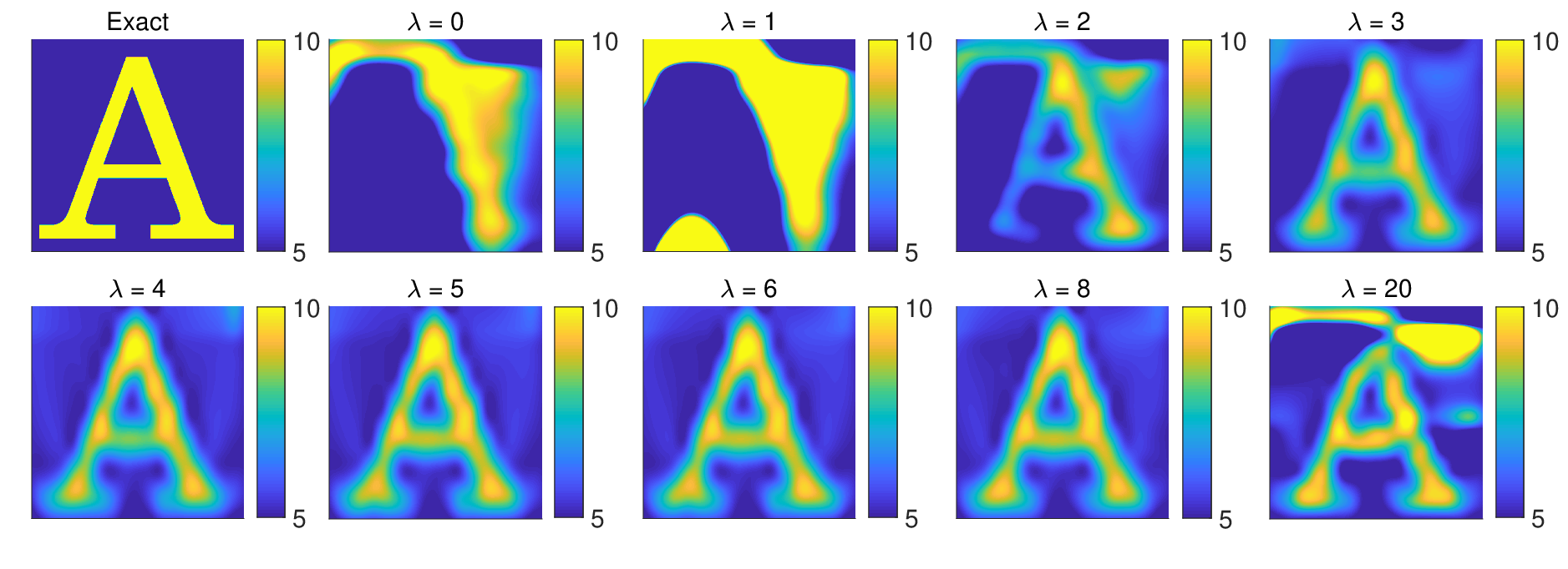
N=3,λ=5.N=3,\lambda=5.
Refer to caption
Figure 2: Test 1. The reconstructed coefficient a⁡(𝐱)a\left(\mathbf{x}\right), where the function μa​(𝐱)\mu_{a}\left(\mathbf{x}\right) is given in ( 6.8) with ca=5c_{a}=5 inside of the letter ‘A’. The goal here is to test different values of the parameter λ=0,1,2,3,4,5,6,8,20\lambda=0,1,2,3,4,5,6,8,20 for N=3N=3. The value of λ\lambda can be seen on the top side of each square. The images have a low quality for λ=0,1,2,3\lambda=0,1,2,3. Then the quality is improved and is stabilized at λ=5\lambda=5. Thus, we select λ=5\lambda=5 as an optimal value of this parameter for all follow up tests. On the other hand, the last image is for the case λ=20.\lambda=20. This image demonstrates that the quality of the reconstructions deteriorates for too large value of λ\lambda.

At last, we want to demonstrate numerically again that N=3N=3 is indeed a good choice of NN for our optimal value of λ=5.\lambda=5. Taking λ=5,\lambda=5, we test the same letter ‘A’ as above with ca=5c_{a}=5 in it, but for N=1,2,3,5,7,12.N=1,2,3,5,7,12. The results are displayed in Figure 3. One can observe that reconstructions have a low quality for N=1,2N=1,2.  Next, the reconstructions are basically the same for N=3,5,7,12.N=3,5,7,12. However, the computational cost increases very rapidly with the increase of NN. Thus, we conclude that to balance between the reconstruction accuracy and the computational cost, we should use N=3N=3, which coincides with the above choice.
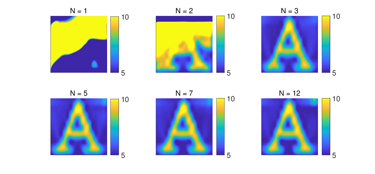
Refer to caption
Figure 3: Test 1. The reconstructed coefficient a⁡(𝐱)a\left(\mathbf{x}\right), where the function μa​(𝐱)\mu_{a}\left(\mathbf{x}\right) is given in (6.8) with ca=5c_{a}=5 inside of the letter ‘A’. We took the optimal value of the parameter λ=5\lambda=5 (see Figure 2) and have tested different values of the parameter N=1,2,3,5,7,12N=1,2,3,5,7,12. A low quality can be observed for N=1,2N=1,2. The reconstructions are basically the same for N=3,5,7,12N=3,5,7,12. However, the computational cost increases very rapidly with the increase of NN. We conclude, therefore, that to balance between the reconstruction accuracy and the computational cost, we should use N=3N=3. Thus, we use below λ=5\lambda=5 and N=3N=3.

Test 2. We test the reconstruction of the coefficient a⁡(𝐱)a(\mathbf{x}) with the shape of the letter ‘A’ where the function μa​(𝐱)\mu_{a}\left(\mathbf{x}\right) is given in (6.8). We test different values of the parameter ca=10,15,20,30c_{a}=10,15,20,30 inside of the letter ‘A’. Thus, by (6.9) the inclusion/background contrasts now are respectively 3:13:1, 4:14:1, 5:15:1 and 6:16:1. The function εr​(𝐱)=εr(1)​(𝐱)\varepsilon_{r}(\mathbf{x})=\varepsilon_{r}^{\left(1\right)}(\mathbf{x}) as in (6.11). Our computational results for this test are displayed on Figure 4. One can observe that the quality of these images is good for all four cases, although it slightly deteriorates for ca=20c_{a}=20 and ca=30c_{a}=30. The computed inclusion/background contrast is accurate, see (6.10) and compare with (6.9).

Refer to caption
Figure 4: Test 2. Exact (top) and reconstructed (bottom) coefficient a⁡(𝐱)a(\mathbf{x}) for ca=10,15,20,30c_{a}=10,15,20,30 (from left to right ) inside of the letter ‘A’ as in (6.8). Thus, by (6.9) the inclusion/background contrasts now are respectively 3:13:1, 4:14:1, 5:15:1 and 6:16:1. The image quality remains basically the same for all these values of the parameter cac_{a}, although a slight deterioration of this quality can be observed for ca=20c_{a}=20 and ca=30c_{a}=30. The computed inclusion/background contrasts (6.9) are reconstructed accurately.

Test 3. We test the reconstruction of the coefficient a⁡(𝐱)a(\mathbf{x}) with the shape of two letters ‘SZ’, where the function μa​(𝐱)\mu_{a}\left(\mathbf{x}\right) is given in (6.8) with ca=5c_{a}=5 inside of each of these two letters, and μa​(𝐱)=0\mu_{a}\left(\mathbf{x}\right)=0 outside of each of these two letters. SZ are two letters in the name of the city (Shenzhen) were the second and the fifth authors reside. The results are displayed on Figure 5.
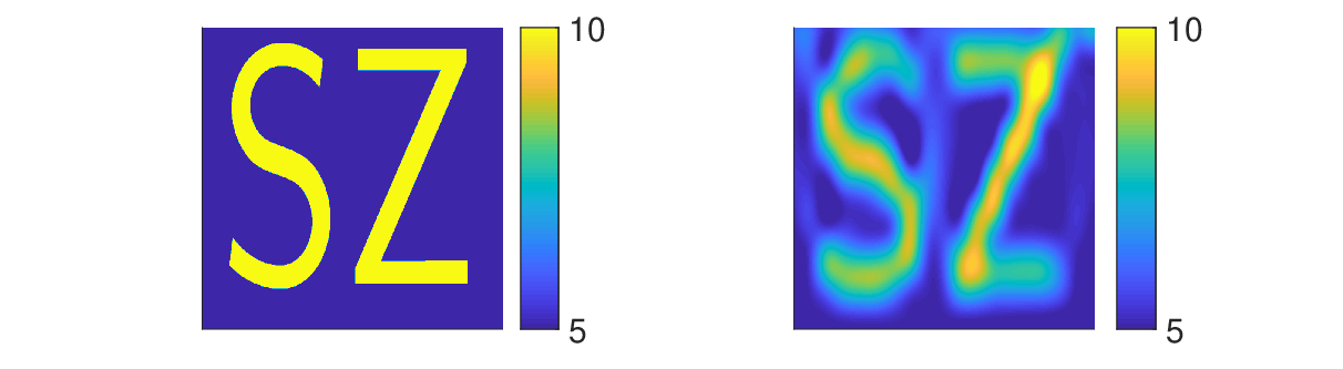
Refer to caption
Figure 5: Test 3. Exact (left) and reconstructed (right) coefficient a⁡(𝐱)a(\mathbf{x}) for the case when the function μa​(𝐱)\mu_{a}\left(\mathbf{x}\right) is given in (6.8) with ca=5c_{a}=5 with the shape of two letters ‘SZ’. In (6.8) ca=5c_{a}=5 inside of each of these two letters and μa​(𝐱)=0\mu_{a}\left(\mathbf{x}\right)=0 outside of each of these two letters. Here N=3,λ=5N=3,\lambda=5. The quality is good and the computed inclusion/background contrasts are accurately reconstructed in both letters, see (6.9) and ( 6.10).

Test 4. We now use the noisy data as in (6.12) with δ=0.03\delta=0.03 and δ=0.05\delta=0.05, i.e. with 3% and 5% noise level. We test the reconstruction of the coefficient a⁡(𝐱)a(\mathbf{x}) with the shape of either the letter ‘A’ or the letter ‘Ω\Omega’, where the function μa​(𝐱)\mu_{a}\left(\mathbf{x}\right) is given in (6.8) with ca=5c_{a}=5 inside of each of these two letters. The results are displayed on Figure 6. One can observe accurate reconstructions in all four cases. In particular, the inclusion/background contrasts are reconstructed accurately, see (6.10) and compare with (6.9).
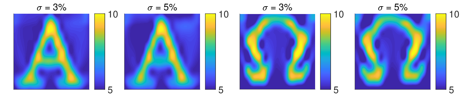
Refer to caption
Figure 6: Test 4. Reconstructed coefficient a⁡(𝐱)a(\mathbf{x}) with the shape of letters ‘A’ and ‘Ω\Omega’ with ca=5c_{a}=5 from noise polluted observation data as in (6.12) with δ=0.03\delta=0.03 and δ=0.05\delta=0.05, i.e. with 3% and 5% noise level. One can observe accurate reconstructions in all four cases. In particular, the inclusion/background contrasts are reconstructed accurately, see (6.9) and (6.10).

References

  • [1] M. Asadzadeh and L. Beilina, A stabilized P1 domain decomposition finite element method for time harmonic Maxwell’s equations, Math. Comput. Simul, 204 (2023), pp. 556–574.
  • [2] A. B. Bakushinskii, M. V. Klibanov, and N. A. Koshev, Carleman weight functions for a globally convergent numerical method for ill-posed Cauchy problems for some quasilinear PDEs, Nonlinear Anal. Real World Appl., 34 (2017), pp. 201–224.
  • [3] G. Bal, Inverse transport theory and applications, Inverse Probl., 25 (2009), p. 053001.
  • [4] G. Bal and A. Jollivet, Generalized stability estimates in inverse transport theory, Inverse Probl. Imaging, 12 (2018), pp. 59–90.
  • [5] G. Bal and A. Tamasan, Inverse source problems in transport equations, SIAM J. Math. Anal., 39 (2007), pp. 57–76.
  • [6] L. Beilina, M. G. Aram, and E. M. Karchevskii, An adaptive finite element method for solving 3D electromagnetic volume integral equation with applications in microwave thermometry, J. Comput. Phys., 459 (2022), p. 111122.
  • [7] L. Beilina and E. Lindstrom, An adaptive finite element/finite difference domain decomposition method for applications in microwave imaging, Electronics, 11 (2022), p. 1359.
  • [8] M. Bellassoued and M. Yamamoto, Carleman estimates and applications to inverse problems for hyperbolic systems, Springer, Japan, 2017.
  • [9] M. Born and E. Wolf, Principles of optics, Cambridge University Press, 7th ed., 1999.
  • [10] A. L. Bukhgeim and M. V. Klibanov, Uniqueness in the large of a class of multidimensional inverse problems, Soviet Math. Doklady, 17 (1981), pp. 244–247.
  • [11] M. Cristofol, S. Li, and Y. Shang, Carleman estimates and some inverse problems for the coupled quantitative thermoacoustic equations by partial boundary layer data. Part II: Some inverse problems, Math. Methods Appl. Sci., published online, (2023), https://doi.org/10.1002/mma.9252.
  • [12] S.-R. Fu and P.-F. Yao, Stability in inverse problem of an elastic plate with a curved middle surface, Inverse Probl., 39 (2023), p. 045003.
  • [13] H. Fujiwara, K. Sadiq, and A. Tamasan, A Fourier approach to the inverse source problem in an absorbing and anisotropic scattering medium, Inverse Probl., 36 (2020), p. 015005.
  • [14] H. Fujiwara, K. Sadiq, and A. Tamasan, Numerical reconstruction of radiative sources in an absorbing and nondiffusing scattering medium in two dimensions, SIAM J. Imaging Sci., 13 (2020), pp. 535–555.
  • [15] H. Fujiwara, K. Sadiq, and A. Tamasan, A source reconstrution method in two dimensional radiative transport using boundary data measured on an arc, Inverse Probl., 37 (2021), p. 115005.
  • [16] G. Giorgi, M. Brignone, R. Aramini, and M. Piana, Application of the inhomogeneous Lippmann–Schwinger equation to inverse scattering problems, SIAM J. Appl. Math., 73 (2013), pp. 212–231.
  • [17] F. Gölgeleyen and M. Yamamoto, Stability for some inverse problems for transport equations, SIAM J. Math. Anal., 48 (2016), pp. 2319–2344.
  • [18] A. V. Goncharsky and S. Y. Romanov, Iterative methods for solving coefficient inverse problems of wave tomography in models with attenuation, Inverse Probl., 33 (2017), p. 025003.
  • [19] A. V. Goncharsky and S. Y. Romanov, A method of solving the coefficient inverse problems of wave tomography, Comput. Math. Appl., 77 (2019), pp. 967–980.
  • [20] J. P. Guillement and R. G. Novikov, Inversion of weighted Radon transforms via finite Fourier series weight approximation, Inverse Probl. Sci. En., 22 (2013), pp. 787–802.
  • [21] E. Hassi, S.-E. Chorfi, and L. Maniar, Stable determination of coefficients in semilinear parabolic system with dynamic boundary conditions, Inverse Probl., 38 (2022), p. 115007.
  • [22] J. Heino, S. Arridge, J. Sikora, and E. Somersalo, Anisotropic effects in highly scattering media, Phys. Rev. E, 68 (2003), p. 03198.
  • [23] V. Isakov, Inverse Problems for Partial Differential Equations, Springer, New York, 2006.
  • [24] S. I. Kabanikhin, N. S. Novikov, I. V. Oseledets, and M. A. Shishlenin, Fast toeplitz linear system inversion for solving two-dimensional acoustic inverse problem, J. Inverse Ill-Posed Probl., 23 (2015), pp. 687–700.
  • [25] S. I. Kabanikhin, K. K. Sabelfeld, N. S. Novikov, and M. A. Shishlenin, Numerical solution of an inverse problem of coefficient recovering for a wave equation by a stochastic projection methods, Monte Carlo Methods Appl., 21 (2015), pp. 189–203.
  • [26] V. A. Khoa, M. V. Klibanov, and L. H. Nguyen, Convexification for a 3D inverse scattering problem with the moving point source, SIAM J. Imag. Sci., 13 (2020), pp. 871–904.
  • [27] M. Klibanov and M. Yamamoto, Exact controllability for the time dependent transport equation, SIAM J. Control Optim., 46 (2007), pp. 2071–2195.
  • [28] M. V. Klibanov, Inverse problems and Carleman estimates, Inverse Probl., 8 (1992), pp. 575–596.
  • [29] M. V. Klibanov, Global convexity in a three-dimensional inverse acoustic problem, SIAM J. Math. Anal., 28 (1997), pp. 1371–1388.
  • [30] M. V. Klibanov, Carleman estimates for global uniqueness, stability and numerical methods for coefficient inverse problems, J. Inverse Ill-Posed Probl., 21 (2013), pp. 477–510.
  • [31] M. V. Klibanov, Convexification of restricted Dirichlet to Neumann map, J. Inverse Ill-Posed Probl., 25 (2017), pp. 669–685.
  • [32] M. V. Klibanov and O. V. Ioussoupova, Uniform strict convexity of a cost functional for three-dimensional inverse scattering problem, SIAM J. Math. Anal, 26 (1995), pp. 147–179.
  • [33] M. V. Klibanov and J. Li, Inverse Problems and Carleman Estimates: Global Uniqueness, Global Convergence and Experimental Data, De Gruyter, 2021.
  • [34] M. V. Klibanov, J. Li, L. Nguyen, and Z. Yang, Convexification numerical method for a coefficient inverse problem for the radiative transport equation, SIAM J. Imag. Sci., 16 (2023), pp. 35–63, https://doi.org/10.1137/22m1509837.
  • [35] M. V. Klibanov, J. Li, and Z. Yang, Convexification for the viscocity solution for a coefficient inverse problem for the radiative transfer equation, arXiv:2302.12474, (2023).
  • [36] M. V. Klibanov and S. Pamyatnykh, Global uniqueness for a coefficient inverse problem for the non-stationary transport equation via Carleman estimate, J. Math. Anal. Appl., 343 (2008), pp. 352–365.
  • [37] M. V. Klibanov and V. G. Romanov, A hölder stability estimate for a coefficient inverse problem for the wave equation with a point source, Eurasian J. Math. Comp., 10(2) (2022), pp. 11–25.
  • [38] R. Y. Lay and Q. Li, Parameter reconstruction for general transport equation, SIAM J. Math. Anal., 52 (2020), pp. 2734–2758.
  • [39] J. Li, H. Liu, and S. Ma, Determining a random schrö dinger operator: both potential and source are random, Commun. Math. Phys., 381 (2021), pp. 527–556.
  • [40] J. Li, H. Liu, L. Rondi, and U. G., Regularized Transformation-Optics Cloaking for the Helmholtz Equation: From Partial Cloak to Full Cloak, Commun. Math. Phys., 335(2) (2015), pp. 671–712.
  • [41] S. R. McDowall, An inverse problem for the transport equation in the presence of a Riemannian metric, Pac. J. Math., 216 (2004), pp. 303–326.
  • [42] R. Novikov and M. Santacesaria, Monochromatic reconstruction algorithms for two-dimensional multi-channel inverse problems, Int. Math. Res. Not., 2013 (2012), pp. 1205–1229.
  • [43] G. Peyre, Toolbox fast marching, MATLAB Central File Exchange, (2023).
  • [44] V. G. Romanov, Inverse Problems of Mathematical Physics, VNU Press, Utrecht, The Netherlands, 1986.
  • [45] V. G. Romanov, Inverse problems for differential equations with memory, Eurasian J. Math. Comp., 2 (2014), pp. 51–80.
  • [46] J. A. Scales, M. L. Smith, and T. L. Fischer, Global optimization methods for multimodal inverse problems, J. Comp. Phys., 103 (1992), pp. 258–268.
  • [47] A. V. Smirnov, M. V. Klibanov, and L. H. Nguyen, On an inverse source problem for the full radiative transfer equation with incomplete data, SIAM J. Sci. Comput., 41 (2019), pp. B929–B952.
  • [48] A. N. Tikhonov, A. V. Goncharsky, V. V. Stepanov, and A. G. Yagola, Numerical methods for the solution of ill-posed problems, Kluwer, London, 1995.
  • [49] M. M. Vajnberg, Variational method and method of monotone operators in the theory of nonlinear equations, Israel Program for Scientific Translations, Jerusalem-London, 1973.
  • [50] M. Yamamoto, Carleman estimates for parabolic equations, Topical Review. Inverse Probl., 25 (2009), p. 123013.