Data–driven modal decomposition methods as
feature detection techniques for flow problems:
a critical assessmentJournal: Journal of LaTeX Templates

B. Begiashvili Email: beka.begiashvili@alumnos.upm.es Address: ETSI Aeronáutica y del Espacio – Universidad Politécnica de Madrid, 28040 Madrid, Spain N. Groun Email: gr.nourelhouda@alumnos.upm.es Address: ETSI Aeronáutica y del Espacio – Universidad Politécnica de Madrid, 28040 Madrid, Spain Address: ETSI Telecomunicación – Universidad Politécnica de Madrid, 28040 Madrid, Spain J. Garicano-Mena Email: jesus.garicano.mena@upm.es Address: ETSI Aeronáutica y del Espacio – Universidad Politécnica de Madrid, 28040 Madrid, Spain Address: Center for Computational Simulation (CCS), 28660 Boadilla del Monte, Spain S. Le Clainche Email: soledad.leclainche@upm.es Address: ETSI Aeronáutica y del Espacio – Universidad Politécnica de Madrid, 28040 Madrid, Spain Address: Center for Computational Simulation (CCS), 28660 Boadilla del Monte, Spain E. Valero Email: eusebio.valero@upm.es Address: ETSI Aeronáutica y del Espacio – Universidad Politécnica de Madrid, 28040 Madrid, Spain Address: Center for Computational Simulation (CCS), 28660 Boadilla del Monte, Spain

Abstract

Modal decomposition techniques are showing a fast growth in popularity for their good properties as data-driven tools. There are several modal decomposition techniques, yet Proper Orthogonal Decomposition (POD) and Dynamic Mode Decomposition (DMD) are considered the most demanded methods, especially in the field of fluid dynamics. Following their magnificent performance on various applications in several fields, numerous extensions of these techniques have been developed. In this work we present an ambitious review comparing eight different modal decomposition techniques, including most established methods: POD, DMD and Fast Fourier Trasform (FFT), extensions of these classical methods: based on time embedding systems, Spectral POD (SPOD) and Higher Order DMD (HODMD), based on scales separation, multi-scale POD (mPOD), multi-resolution DMD (mrDMD), and based on the properties of the resolvent operator, the data-driven Resolvent Analysis (RA). The performance of all these techniques will be evaluated on three different testcases: the laminar wake around cylinder, a turbulent jet flow, and the three dimensional wake around cylinder in transient regime. First, we show a comparison between the performance of the eight modal decomposition techniques when the datasets are shortened. Next, all the results obtained will be explained in details, showing both the conveniences and inconveniences of all the methods under investigation depending on the type of application and the final goal (reconstruction or identification of the flow physics). In this contribution we aim on giving a -as fair as possible- comparison of all the techniques investigated. To the authors knowledge, this is the first time a review paper gathering all this techniques have been produced, clarifying to the community what is the best technique to use for each application.

Keywords:

modal decompositions, proper orthogonal decomposition, dynamic mode decomposition, matrix factorization , turbulent flows, laminar flows , transient flows, flow reconstruction, machine learning, feature detection, low order algorithms.

1 Introduction

Nowadays, modal decomposition techniques have shown a fast growth in popularity in several fields and applications (aerospace and wind engineering, oil and gas industry, medicine…). These types of techniques have become very popular in the field of fluid dynamics, as they grant the understanding of complex flows as well as allowing the reconstruction of diverse, useful information related to the flow physics.
In fluid mechanics there are two relevant modal decomposition techniques due to their tested good performance in a wide range of applications: Proper Orthogonal Decomposition (POD) and Dynamic Mode Decomposition (DMD). Several authors put a great effort in increasing the robustness of these methods with the aim also at widening their range of applications, hence they develop new variants and extensions of DMD and POD methods. To name a few: (i) snapshot POD [1, 2], this algorithm, which is based on the use of snapshots, can be said to be an exact symmetry of classic POD [3], as it involves correlations in time and averaging in space, in contrast to the classic POD, which has correlations in space and averaging in time. When compared to classical POD, which has limitations because of computational intensiveness, snapshot POD is sufficiently fast and computationally efficient. (ii) Extended POD (EPOD) [4], which is a generalization of the standard POD, where it uses the temporal basis of one variable to find the modes of any data ensemble synchronized with the data ensemble used for the decomposition. This method have been mainly used, and found efficient in extracting information on correlated events and (iii) cross POD (CPOD)[5], a quite recent extension of the classical POD. The technique, which was developed in order to optimally decompose the trace of cross-covariances of flow fluctuations, decomposes the flow in terms of modes that are ranked according to the cross correlation they carry. This technique shows a promising direction in the application to generalized Reynolds stresses. Regarding improvements of the classical DMD, we mention the following: (i) extended DMD (EDMD)[6], which ameliorates the standard DMD by including a dictionary of observables, which spans a finite dimensional subspace on which we can approximate the Koopman operator and this will allow the method to capture more complex behavior. (ii) Sparsity promoting DMD (spDMD)[7], which uses sparse estimation and convex optimization techniques in order to end up with fewer, but more important modes and (iii) DMD with control (DMDc)[8], where this technique employs both measurements of the system and an orthogonal complement of control inputs to extract the underlying dynamics.
In this contribution we are presenting a review comparing eight modal decomposition techniques, which can be categorized into three groups: (i) classical methods including Proper Orthogonal Decomposition (POD) [1], Dynamic Mode Decomposition (DMD) [9] and Fast Fourier Transform (FFT) [10], (ii) improved methods based on time-embedding systems: Spectral Proper Orthogonal Decomposition (SPOD) [11] and Higher Order Dynamic Mode Decomposition (HODMD) [12] and (iii) multi-resolution methods capable to differentiate fast and slow scales: multi-scale POD (mPOD) [13] and multi-resolutional DMD (mrDMD) [14]. Finally we close with the latest modal decomposition technique, the Resolvent Analysis method (RA) [15], with the aim at showing the similarities between the resolvent modes and the DMD and POD modes. To the authors’ knowledge, this is the first time all these techniques have been investigated and compared in one review paper. However, our objective is not to describe all the methods in details, but to make explicit the undefined framework underlying those methods.
These methods have been selected due to their strong potential for patterns identification in a wide range of applications. For instance, the POD for example was one of the first techniques to be employed in the field of fluid mechanics, where it was introduced in the context of turbulence by Lumley in 1967 [16, 17] and continued to cover numerous application till this day. Smith et al. [18] used POD to build low-dimensional models for turbulent fluid flows. Willcox et al. [19] combined POD with concepts from balanced realization theory [20], for the reduction of high-order systems, including a CFD model that describes the unsteady linearized motion of a two-dimensional airfoil. Zhang et al. [21] leveraged POD to study the internal unsteady flow structure in a centrifugal pump for its advantages on turbulence analysis.
Another well-known technique is the DMD. Right after introducing the DMD algorithm in 2010, Schmid et al. [22] published a new work in order to demonstrate the potential of the DMD technique, where they showed the robustness of their technique on two examples: (i) the decomposition of Schlieren snapshots of a helium jet and (ii) the decomposition of time-resolved PIV-measurements of an unforced and forced jet. Rowely et al. [23] aimed to describing the global behavior of complex nonlinear flows using the spectral analysis of the Koopman operator, where they recruit the DMD to find the Koopman modes. The results demonstrated the capacity of the technique in capturing the dominant frequencies and elucidating the associated spatial structures. Kutz et al. [24] produced a detailed, information rich book on the DMD algorithm. The book developed the fundamental theoretical foundations of DMD and highlighted many of its applications. A few years earlier, Garicano-Mena et al. [25] have also used the DMD algorithm to investigate both standard and actuated turbulent channel databases generated by Direct Numerical Simulation (DNS), in order to explore the existence of flow features linked to drag reduction and the possibility of learning how those structures could be modified to better understand the efficiency of drag reduction strategies if they did exist. With a different approach, Barros et al. [26] worked on enabling DMD to extract features from observations with different mesh topologies and dimensions, such as those found in adaptive mesh refinement/coarsening (AMR/C) simulations, as well as evaluating the DMD efficiency to reconstruct the dynamics and some relevant quantities of interest.
Similarly, extensions of the previously mentioned techniques are quite popular as well. A recent extension of POD is Spectral POD (SPOD), which was developed in order to overcome the difficulties classical POD faces when the relevant coherent structures occur at low energies or at multiple frequencies, which is often the case. This algorithm, which can be applied to both spatially and temporally resolved data, has already covered several applications in fluid dynamics. Shahram et al. [27] employed SPOD to study the spatio-temporal dynamics of the coherent structures in an under-expanded supersonic impinging jet, where the SPOD decomposes the flow filed allowing the illustration of the forward and backward paths of the feedback loop, representing two things: (i) the hydrodynamic instability in the shear layer of the jet and (ii) the acoustic wave propagating in the medium. Leandra et al. [28] also used SPOD to identify energetically dominant coherent structures in turbulent pipe flows, using direct numerical simulations, performed with a high-order spectral-element method. Meanwhile Akhil et al. [29] used a large-eddy simulation data of a turbulent jet to demonstrate the applicability of the SPOD algorithm in four different application: low-rank reconstruction, denoising, frequency–time analysis and prewhitening. All the approached strategies of this work gave satisfactory results.
Higher order dynamic mode decomposition (HODMD), is also a recent extension of one of the most known modal decomposition techniques, the DMD. Even though it has been only five years since this algorithm was developed, it has covered several applications in the fluid dynamics field [30] and even reached biology [31] and the medical field [32, 33]. Le Clainche et al. [12] have demonstrated the efficiency of the HODMD algorithm on several applications including studying the flow structures of a zero-net-mass-flux (ZNMF) jet [34], analyzing turbulent flow of an elastoviscoplastic fluid [35] and to identify cross-flow instabilities [36]. Similarly, Méndez et al. [37] introduced a new data processing method, based on HODMD, to analyze actual flight test experimental data. Their proposed technique provides useful and interesting information for predicting flutter and proved to be suitable for the analysis of flight test data in real time.

Multi-scale POD (mPOD) [13] and multi-resolution DMD (mrDMD) [14] have also become very popular during the last days. Tang et al. [38] investigated the response of the large- and small-scale structures on the dynamic cylindrical element using mPOD, where after employing the mPOD for data processing, the modes obtained by the technique were used to construct the large- and small-scale structures. Procacci et al. [39] examined the flow field dynamics of bluff-body stabilized swirling and non-swirling flames using the mPOD algorithm. By applying this method, they were able to identify the main flow patterns in the velocity field and isolate coherent structures linked to various flow instabilities. Esposito et al. [40] used the mPOD technique for the analysis of cavitation instabilities in water and liquid nitrogen. In this work, the authors highlighted the advantage of the mPOD in providing band-limited modes preserving anyway a good convergence unlike standard POD. Climaco et al. [41] proposed an approach for damage detection in wind turbine gearboxes using the mrDMD technique. Gearbox vibration signals generated under varying load conditions were analyzed using mrDMD, which resulted the identification of important features related to the damage. Gonzales et al. [42] created a continuous-time model of the pressure profile over the fluttering airfoil using mrDMDin order to provide a higher temporal resolution information about the system. The mrDMD algorithm was able to isolate the behavior of an oscillating shock wave over the surface of the fluttering airfoil, as well as determine the frequency of the amplitude oscillations of the shock wave.
The last technique we discuss is the Resolvent Analysis (RA). Before developing the data-driven RA by Herrmann et al. in 2021 [43], the RA was already making an impact in the field of fluid mechanics, trying to conduct reserach towards new applications of flow control [15, 44]. Luhar et al. [45] reformulated the resolvent analysis to generate predictions for the fluctuating pressure field in turbulent pipe flow. They used their proposed approach to show how the obtained response modes reconcile many of the key relationships among the velocity field, coherent structures and high-amplitude wall-pressure events. Yeh et al. [46] employed the RA to design active control techniques for separated flows over an airfoil. They also considered the use of a temporal filter to limit the time horizon and conducted a global resolvent analysis on the baseline turbulent mean flows to identify the actuation frequency and wavenumber that provide large perturbation energy amplification (see also [47, 48]).

The rest of the work is organized as follows: Section 2 summarizes algorithms for these different techniques. Section 3 introduces and describes the test cases we are evaluating the algorithms on. A comparison to test the convergence of the method as function of the number of snapshots is presented in Section 4, followed by the main, detailed results, which are presented in Section 5. Finally, Section 6 presents main conclusions of the work.

2 Methodology

In this section we present the different data analysis methods considered in this work. Those methods can be immediately separated into two major, distinct categories: POD-related methods and DMD-related methods. Regarding the upcoming discussion, however, one should bear in mind that strong connections exist between the methods inside a given category. Moreover, links can also be established between both families of methods. These relationships are perhaps better revealed if one resorts to matrix factorization based interpretations of the algorithms, see e.g. in Refs. [9, 49].

Consider a sequence of $n_{p}$ -dimensional instantaneous flow fields $\mathbf{v}_{j}$ , (e.g., system states, snapshots or frames) indexed from $1$ to $n_{t}$ and that have been acquired at the uniform sampling rate $\Delta t^{s}=t_{j+1}-t_{j}$ . Note that $n_{p}$ accounts for the number of spatial locations $n_{s}$ (grid points, pixels) and the number of flow variables considered $n_{vars}$ (velocity components, pressure, …), so that $n_{p}=n_{s}\times n_{vars}$ ; by reshaping the snapshots as column vectors $\mathbf{v}_{j}\in\mathbb{R}^{n_{p}}$ , a data matrix is constructed:

\displaystyle\mathbf{V}_{1}^{n_{t}}=\left[\mathbf{v}_{1},\,\mathbf{v}_{2},\,\ldots,\,\mathbf{v}_{n_{t}-1},\,\mathbf{v}_{n_{t}}\right]\in\mathbb{R}^{n_{p}\times n_{t}}.

(1)

Most fluid dynamics applications, be these numerical or experimental, lead to data matrices with $n_{t}\ll n_{p}$ , termed Tall & Skinny (TS) matrices. Notation-wise, we will often omit the sub and superindexes for the data matrix whenever they are clear from the context.

It is not uncommon to consider the associated dataset obtained by subtracting from each of the temporal snapshots the temporally averaged field, this is, the mean flow, i.e. $\bar{\mathbf{v}}=\frac{1}{n_{t}}\sum\limits_{j=1}^{n_{t}}\mathbf{v}_{j}$ . Context often determines whether the original or the average-subtracted dataset are being considered, and hence we maintain the notation $\mathbf{V}_{1}^{n_{t}}$ for both.

Before dwelling into the specifics of the different methods considered, we recall that most data–driven modal analysis techniques can be interpreted as matrix factorization strategies (see [9, 49, 50], but also [13]), as in:

\displaystyle\mathbf{V}_{1}^{n_{t}}=\mathbf{A}\,\mathbf{B}\,\mathbf{C}^{H}=\sum\limits_{j=1}^{r}b_{j}\,\mathbf{a}_{j}\cdot\mathbf{c}_{j}^{H},

(2)

where $\mathbf{A}\in\mathbb{C}^{n_{p}\times r}$ ^*^* * Most POD-related methods factorize the data matrix into real factors, whereas DMD-related methods yield complex factors. Those complex factors form nevertheless balanced complex-conjugated variable pairs, so that the real data matrix $\mathbf{V}_{1}^{n_{t}}$ is recovered., $\mathbf{B}\in\mathbb{C}^{r\times r}$ , $\mathbf{C}\in\mathbb{C}^{n_{t}\times r}$ and $H$ is the complex-conjugate operator. A diagonal structure is usually enforced for $\mathbf{B}$ , and the dimension $r$ is chosen so that $1\leq r\leq\min(n_{p},\,n_{t})$ . Since $\mathbf{a}_{j}\in\mathbb{C}^{n_{p}}$ , matrix $\mathbf{A}$ is related to the spatial dimension of the dataset and thus $\mathbf{A}$ is sometimes referred as the topos matrix. In the same manner, $\mathbf{c}_{j}\in\mathbb{C}^{n_{t}}$ , and thus related to the temporal dimension; matrix $\mathbf{C}$ is called accordingly the chronos matrix.

In what follows, we review first the basic POD, DMD and FFT techniques, stressing out the connections between them. Next, we address several extensions of those methods. The first extension leverages data redundancy either in the spectral domain, by averaging spectra from shorter subsequences (in the spirit of the Welch method [51]), or in the temporal domain through time–lagging of the data snapshots; in both cases, improved analysis techniques are obtained. Spectral Proper Orthogonal Decomposition [11] and Higher Order Dynamic Mode Decomposition [12] are representatives of this approach. Next, a multi–scale approach for POD, and a multi–resolution interpretation of DMD are introduced. Finally, resorting to an input–output perspective in the space of states [52] allows to introduce the data–driven, DMD–based Resolvent Analysis (RA) technique described in [43].

Table 1 lists the different methods analyzed in this contribution. For each, one or two fundamental references are provided. The table also credits the origin of the implementations for the different methods, at least when it is available.

Table 1: Summary of the data–analysis methods considered in this work, principal references and availability.

Method Major references Available from POD [53, 54] Matlab commands svd, eig DMD [9, 55] http://www.ece.umn.edu/users/mihailo/software/dmdsp/ FFT [10, 50] Matlab native commands fft, fft2 SPOD [11, 56] https://nl.mathworks.com/matlabcentral/fileexchange/65683-spectral-proper-orthogonal-decomposition-spod HODMD [12, 57] https://short.upm.es/q8rip mPOD [13, 58] https://github.com/mendezVKI/MODULO mrDMD [14, 49] https://github.com/kdmarrett/dmd RA [43] N.A./Own implementation

2.1 The Proper Orthogonal Decomposition methods

We begin this necessarily brief review of classical Proper Orthogonal Decomposition methods by acknowledging that many related methods are referred to as POD in the bibliography. Principal Component Analysis or Karhunen-Loève decomposition are also terms applied to these techniques.

Reference [53] presents a good, integrative description of three different yet interrelated POD algorithms. We cover here two of them, as they will be useful in the posterior discussion.

A first strategy consists in the direct application of the (economy–sized) Singular Value Decomposition (SVD) to the average substracted dataset:

\displaystyle\mathbf{V}_{1}^{n_{t}}\overset{SVD}{=}\mathbf{L}_{0}\;\mathbf{S}_{0}\;\mathbf{R}_{0}^{T}=\sum\limits_{j=1}^{r}s_{0,j}\,\mathbf{l}_{0,j}\cdot\mathbf{r}_{0,j}^{T}.

(3)

Matrix $\mathbf{S_{0}}$ contains as diagonal entries the non–negative and decreasing singular values $s_{0,j}$ , whereas the real matrices $\mathbf{L}_{0}$ and $\mathbf{R}_{0}$ , which are orthogonal, have as their columns $\mathbf{l}_{0,j}$ and $\mathbf{r}_{0,j}$ the left and right singular vectors. Note that superindex $T$ stands for the transposition operator. Following Refs. [59, 9, 55, 60], the left singular vectors $\mathbf{l}_{0,j}$ are identified with the POD modes.

The second strategy, which for historical reasons is termed the method of snapshots [1], considers the temporal correlation matrix $\mathbf{K}\equiv\left(\mathbf{V}_{1}^{n_{t}}\right)^{T}\;\mathbf{V}_{1}^{n_{t}}$ , and its eigenvalue decomposition:

\displaystyle\mathbf{K}\;\mathbf{R}_{0}=\mathbf{R}_{0}\;\mathbf{D}_{s^{2}},

(4)

where the singular values are retrieved as the square root of the diagonal entries of $\mathbf{D}_{s^{2}}$ , i.e., $s_{0,j}=\sqrt{D_{s^{2},j,j}}$ , and the POD modes are given by:

\displaystyle\mathbf{L}_{0}=\mathbf{V}_{1}^{n_{t}}\,\mathbf{R}_{0}\,\mathbf{D}_{s^{2}}^{-1/2}.

(5)

Observe how the data matrix factorization given by Eq. (3) allows to somehow separate the spatial components from the temporal components of the database. Accordingly, one can define the scaled chronos matrix as:

\displaystyle\mathcal{C}_{1}^{n_{t}}\equiv\mathbf{S}_{0}\,\mathbf{R}_{0}^{T}=\sum\limits_{j=1}^{r}\,s_{0,j}\,\mathbf{e}_{j}\cdot\mathbf{r}_{0,j}^{T},

(6)

where $\mathbf{e}_{j}$ is the $j$ -th unit vector in $\mathbb{R}^{r}$ . This matrix will be useful when presenting the Higher Order DMD method in § 2.4.2.

Finally, we point out that the non–increasing singular values in $\mathbf{S}_{0}$ have a relationship with the Frobenius norm of $\mathbf{V}_{1}^{n_{t}}$ , namely $\|\mathbf{V}_{1}^{n_{t}}\|_{F}=\sqrt{\sum_{j}s_{0,j}^{2}}$ . Note also that the upper summation limit in Eq. (3) needs to be $r=\min{(n_{p},n_{t})}$ . The properties of the SVD decomposition [53], guarantee that choosing $1\leq r^{\prime}\leq r$ leads to the $r^{\prime}$ -rank optimal representation of the dataset. The $r^{\prime}$ parameter, often referred to as spatial complexity [61], can be chosen either directly (simply by specifying an integer value), or indirectly, i.e., adjusting $r^{\prime}$ in order to meet a given tolerance $\varepsilon$ , as in:

\displaystyle\frac{\|\mathbf{V}_{1}^{n_{t}}-\sum\limits_{j=1}^{r^{\prime}}s_{0,j}\,\mathbf{l}_{0,j}\cdot\mathbf{r}_{0,j}^{T}\|_{F}}{\sqrt{\sum\limits_{j=1}^{r}s_{0,j}^{2}}}=\sqrt{\frac{\sum\limits_{j=r^{\prime}}^{r}s_{0,j}^{2}}{\sum\limits_{j=1}^{r}s_{0,j}^{2}}}\leq\varepsilon.

(7)

2.2 The Dynamic Mode Decomposition method

The first implementations of the, now established, Dynamic Mode Decomposition methods can be traced back to Ref. [62] (the companion–matrix DMD of Rowley et al.) and to Refs. [9, 63] (the similarity–transformation DMD of Schmid). In this work, and for brevity, we consider mainly implementations derived from the work of Ref. [9]. The classical DMD method assumes a linear relationship between consecutive snapshots

\displaystyle\mathbf{v}_{k+1}=\mathcal{A}^{h}\,\mathbf{v}_{k},

(8)

where the linear operator $\mathcal{A}^{h}$ can be interpreted as a state transition matrix in discrete time [52]. Eq. 8 is sometimes termed the Koopman assumption [57]. Defining the partial subsequences $\mathbf{X}\equiv\mathbf{V}_{1}^{n_{t}-1}$ and $\mathbf{Y}\equiv\mathbf{V}_{2}^{n_{t}}$ , allows to write the former in compact form:

\displaystyle\mathbf{Y}=\mathcal{A}^{h}\;\mathbf{X}.

(9)

Next, SVD of the first subsequence is performed, $\mathbf{X}\overset{SVD}{=}\mathbf{L}_{0}\;\mathbf{S}_{0}\;\mathbf{R}_{0}^{T}$ , cf. Eq. (3), and recall that, at this stage, one could consider a reduced representation of the input data subsequence $\mathbf{X}$ simply by retaining $r^{\prime}\leq r=n_{t}-1$ singular values, according to Eq. (7).

Using the SVD of the $\mathbf{X}$ matrix into Eq. (9) allows to build a reduced matrix $\bar{\mathbf{A}}$ , defined as:

\bar{\mathbf{A}}\equiv\mathbf{L}_{0}^{T}\,\mathcal{A}^{h}\,\mathbf{L}_{0}=\mathbf{L}_{0}^{T}\,\mathbf{Y}\,\mathbf{R}_{0}\,\mathbf{S}_{0}^{-1}.

(10)

The reduced matrix $\bar{\mathbf{A}}$ is the projection of the matrix $\mathcal{A}^{h}$ onto the space linearly generated by the columns of $\mathbf{L}_{0}$ [9]. The DMD method operates under the assumption that the projected matrix $\bar{\mathbf{A}}$ conveys most of the information codified into operator $\mathcal{A}^{h}$ .

Once the reduced matrix $\bar{\mathbf{A}}$ has been calculated, its (right) eigenvalue decomposition:

\displaystyle\bar{\mathbf{A}}\;\boldsymbol{\Psi}=\boldsymbol{\Psi}\;\boldsymbol{\Lambda}_{\mu},

(11)

offers the reduced DMD modes $\boldsymbol{\psi}_{i}$ as the columns of $\boldsymbol{\Psi}$ ; the corresponding eigenvalues $\mu_{i}$ (the diagonal entries of $\boldsymbol{\Lambda}_{\mu}$ ) indicate the temporal growth rates ( $\sigma_{i}=\mathrm{Re}(\mu_{i})$ ) and angular pulsation ( $\omega_{i}=\mathrm{Im}(\mu_{i})$ ).

The projected eigenmodes (namely, the dynamic modes) of matrix $\mathcal{A}^{h}$ are recovered as $\boldsymbol{\Phi}=\mathbf{L}_{0}\,\boldsymbol{\Psi}$ .

Note also that the growth rates and frequencies in the complex half-plane can be recovered from the eigenvalues as:

\displaystyle\lambda_{i}=\log(\mu_{i})/\Delta t^{s}.

(12)

Finally, note that the DMD decomposition allows to reconstruct the original data sequence as:

\displaystyle\mathbf{v}(t_{j})=\sum_{i=1}^{r}\alpha_{i}\,\boldsymbol{\phi}_{i}\mu_{i}^{j\,\Delta\,t^{s}},

(13)

expression that can be recast in matrix form as:

\displaystyle\mathbf{X}=\boldsymbol{\Phi}\,\mathbf{D}_{\alpha}\,\mathbf{V}_{\mu},

(14)

where $\mathbf{V}_{\mu}$ is a Vandermonde matrix whose columns are generated by the successive powers of the column vector $\left[\mu_{1}^{j},\ldots,\mu_{r}^{j}\right]^{T}$ , with $j=0,\ldots,n_{t}-1$ ; and $\mathbf{D}_{\alpha}$ is a diagonal matrix whose non-zero entries are to be determined. There are several strategies available to identify $\mathbf{D}_{\alpha}$ ; we defer the discussion and comparison to § A. Regarding Eq. (13), note that if an upper limit $r^{\prime\prime}\leq r^{\prime}\leq r$ is considered, the original data $\mathbf{X}$ is not reconstructed, but approximated. The parameter $r^{\prime\prime}$ is termed the spectral complexity [61], and can also be tuned directly or indirectly through an $\varepsilon$ -condition similar to that in Eq. (7).

We review now an alternative definition of the DMD method that eases the connection with the Higher Order DMD method discussed in § 2.4.2. This formulation, that follows [12], establishes the Koopman assumption on subsequences built from the scaled chronos matrix, namely:

\displaystyle\mathcal{C}_{2}^{n_{t}}=\mathcal{A}_{1}^{h}\,\mathcal{C}_{1}^{n_{t}-1}.

(15)

The usual procedure is then applied, i.e., the first subsequence is decomposed as $\mathcal{C}_{1}^{n_{t}-1}\overset{SVD}{=}\mathbf{L}_{1}\,\mathbf{S}_{1}\,\mathbf{R}_{1}^{T}$ , and so on. The only difference is that the dynamic modes are now recovered as $\boldsymbol{\Phi}=\mathbf{L}_{0}\,\mathbf{L}_{1}\,\boldsymbol{\Psi}$ . This alternative formulation allows to retrieve the DMD analysis at a reduced computational cost, provided the SVD decomposition is already available, [64, 32].

At this point, we can make a first comparison between the POD and the DMD factorizations, according to the factorization model $\mathbf{V}_{1}^{n_{t}}=\mathbf{A}\,\mathbf{B}\,\mathbf{C}$ of Eq. 2. The methods differ in the nature of the respective topoi matrices: the POD modes $\mathbf{L}_{0}$ are orthogonal to each other, whereas the DMD modes $\boldsymbol{\Phi}$ are not necessarily so. The POD chronos matrix $\mathbf{R}_{0}$ contains all the range of frequencies present in the problem analyzed (i.e., frequencies are mixed), whereas each of the rows of the DMD $\mathbf{V}_{\mu}$ matrix represents a sinusoidal temporal variation at a distinct frequency $\omega_{j}$ : these rows are therefore orthogonal in time. Finally, we insist on the fact that the singular values $s_{0,j}$ are non–increasing, and have a direct relationship with the Frobenius norm of $\mathbf{V}_{1}^{n_{t}}$ , whereas the amplitudes $\alpha_{j}$ do not. In A we comment on the different strategies of computing and selecting the amplitudes.

2.3 Fourier analysis

As discussed in, e.g. Refs. [65, 50], the Discrete Fourier Transform (DFT) of the average-subtracted dataset $\mathbf{V}_{1}^{n_{t}}$ is formally computed as the matrix–matrix product:

\displaystyle\hat{\mathbf{V}}=\mathbf{V}_{1}^{n_{t}}\,\mathcal{F},

(16)

where matrix $\mathcal{F}\in\mathbb{C}^{n_{t}\times n_{t}}$ is a hermitian matrix ( $\mathcal{F}^{H}=\mathcal{F}$ ) generated from the $n_{t}$ roots of unity. Matrix $\mathcal{F}$ has a special structure that can be exploited to efficiently compute the transformation using a Fast Fourier Transform method [10, 50]. Note also that, if a SVD of the dataset is available, the FFT can be applied to the scaled chronos matrix.

In this work, we consider the Power Spectral Density (PSD) of time-resolved datasets, computed as:

\displaystyle PSD=\hat{\mathbf{V}}\odot\hat{\mathbf{V}}^{H},

(17)

where $\odot$ represents the Hadamard (elementwise) product.

The Fourier transformation of the dataset also opens the way to conduct manipulations in the spectral space, which is at the root of both Spectral POD and multi-scale POD methods: these connections will be stressed in the corresponding sections. Regarding DMD, Rowley et al. established that conducting DMD on the average-subtracted dataset is equivalent to DFT [66].

2.4 Improving accuracy through redundancy: window-shift methods

Analyzing the power spectral density of a infinitely long, periodic signal using DFT techniques becomes easier as longer and longer temporal sequences are available. In practice, however, seldom can signals be sampled for long enough. Moreover, spectral estimates do not converge as the number of samples $n_{t}$ is increased: the uncertainty of the estimate at each frequency is as large as the magnitude of the estimate itself.

One strategy to obtain converged estimates averages spectra over several realizations of the signal, using e.g. the Welch method [51]. This strategy is at the root of the Spectral Proper Orthogonal Decomposition (SPOD) method [11]. An equivalent effect can be obtained by resorting to the analysis of $d$ time-lagged snapshots, as done by the Higher Order Dynamic Mode Decomposition (HODMD) method [12, 57]. We review both methods next.

2.4.1 The Spectral Proper Orthogonal Decomposition method

Spectral Proper Orthogonal Decomposition is a spatio-temporal decomposition for statistically stationary data that relies on estimating first, and factorizing next the cross–spectral density (or CSD) tensor at different frequencies. In this work we limit ourselves to a succinct description of the SPOD method, mostly from the algorithmic point of view; Refs. [11, 56] provide a detailed account of the method and its application. As a final comment, note that other data processing strategies also termed SPOD have been described in the literature, e.g. [67, 68], but we do not cover them here.

Refer to caption — Figure 1: Schematic depiction of the method described in [11] for estimating SPOD modes.

Fig. 1 is illustrative of the SPOD algorithm. Estimates of the CSD tensor at a predefined set of frequencies $f_{k}$ can be obtained simply by subdividing the dataset into $n_{b}$ subsequences –or blocks– of temporal length $n_{t}^{\prime}$ , $\mathbf{V}^{b}=\mathbf{V}_{k}^{k+n_{t}^{\prime}}$ , with $1\leq k\leq n_{t}-n_{t}^{\prime}$ and $b=1,\ldots,n_{b}$ . Each of these blocks, which might share (overlap) with neighbouring blocks up to $n_{o}$ snapshots^†^† † Parameter $n_{o}$ is usually chosen so that a 50% overlap between consecutive subsections is attained, [56], is Fourier transformed to $\mathbf{\hat{V}}^{b}$ .

By observing that the $k$ -th column for any of the transformed blocks $\mathbf{\hat{V}}^{b}$ is related to the same frequency $f_{k}$ (see Fig. 1, it is possible to estimate the CSD tensor at $f_{k}$ simply by grouping all those columns into a matrix $\mathbf{V}_{f_{k}}$ and operating:

\mathbf{S}_{f_{k}}=\mathbf{V}_{f_{k}}^{H}\;\mathbf{W}\;\mathbf{V}_{f_{k}}.

(18)

The formulation admits a weight matrix $\mathbf{W}$ that may serve to account for mesh stretching and/or window functions [53, 11]. In this work, we use the Hamming window function [56]. Note that the frequencies $f_{k}$ are defined a priori by the choice of $n_{b}$ and $n_{o}$ , see e.g. Eq. 3.5 in [11]

The SPOD modes are obtained from the eigenvalue decomposition, cf. Eqs. (4) and (5):

\displaystyle\mathbf{S}_{f_{k}}\,\boldsymbol{\Theta}_{f_{k}}=\boldsymbol{\Theta}_{f_{k}}\,\boldsymbol{\Lambda}_{f_{k}},\mbox{ followed by }\mathbf{L}_{0,f_{k}}=\mathbf{V}_{f_{k}}\,\boldsymbol{\Theta}_{f_{k}}\,\boldsymbol{\Lambda}_{f_{k}}^{-1/2}.

(19)

Thus, the SPOD method follows the algorithmic strategy of Eq. 4. As such, the modal energies at the frequency $f_{k}$ is given by the diagonal entries of ${\Lambda}_{f_{k}}^{1/2}$ . Those modal energies are non–increasing, and thus enable sorting the contribution of the different SPOD modes.

2.4.2 The Higher Order Dynamic Mode Decomposition method

The Higher Order DMD method (HODMD) leverages also the notion of redundancy, but in time. The interested reader can consult the extensive bibliography on the topic, e.g. Refs. [12, 34] or the monograph Ref. [57].

In order to introduce the HODMD, the Koopman assumption of Eq. 8 is extended to include $d$ time--lagged snapshots^‡^‡ ‡ Subindex $1$ and superindex $h$ has been removed from the operator $\mathcal{A}^{h}_{1,j}$ to ligthen the notation.:

\displaystyle\mathbf{v}_{k+1}=\sum\limits_{j=1}^{d}\mathcal{A}_{j}\,\mathbf{v}_{k-j}.

(20)

This relation is sometimes termed the higher order Koopman assumption. For reasons of computational efficiency, it is better to write Eq. 20 in terms of the columns of the scaled chronos matrix:

\displaystyle\mathbf{c}_{k+1}=\sum\limits_{j=1}^{d}\mathcal{A}_{j}\,\mathbf{c}_{k-j}.

(21)

Note how setting $d=1$ in either Eq. 20 or (21) leads to the classical DMD method. The matrix counterpart of Eq. 21, see Fig. 2:

\mathbf{C}_{d+1}^{n_{t}}=\mathcal{A}_{1}\mathbf{C}_{1}^{n_{t}-d}+\mathcal{A}_{2}\mathbf{C}_{2}^{n_{t}-d+1}+\ldots+\mathcal{A}_{d}\mathbf{C}_{d}^{n_{t}-1},

(22)

Mathematical manipulations lead to a relation based on a companion-like block matrix:

\begin{bmatrix}\mathbf{C}_{2}^{n_{t}-d+1}\\ \mathbf{C}_{3}^{n_{t}-d+2}\\ \vdots\\ \mathbf{C}_{d}^{n_{t}-1}\\ \mathbf{C}_{d+1}^{n_{t}}\end{bmatrix}=\begin{bmatrix}0&\mathbf{I}&0&\ldots&0\\ 0&0&\mathbf{I}&\ldots&0\\ \vdots&\vdots&\vdots&\ddots&\vdots\\ 0&0&0&\ldots&\mathbf{I}\\ \mathcal{A}_{1}&\mathcal{A}_{2}&\mathcal{A}_{3}&\ldots&\mathcal{A}_{d}\end{bmatrix}\;\begin{bmatrix}\mathbf{C}_{1}^{n_{t}-d}\\ \mathbf{C}_{2}^{n_{t}-d+1}\\ \vdots\\ \mathbf{C}_{d-1}^{n_{t}-2}\\ \mathbf{C}_{d}^{n_{t}-1}\end{bmatrix},

(23)

which can be written compactly as:

\widetilde{\mathbf{C}}_{2}^{n_{t}-d+1}=\widetilde{\mathbf{A}}\;\widetilde{\mathbf{C}}_{1}^{n_{t}-d}.

(24)

Note how this last equation is formally similar to Eq. (15). Indeed, from here on the HODMD follows the classical DMD algorithm. Accordingly, matrix $\widetilde{\mathbf{A}}$ is never explicitly formed; the algorithm proceeds instead by the SVD:

\widetilde{\mathbf{C}}_{1}^{n_{t}-d}\overset{SVD}{=}\widetilde{\mathbf{L}}_{1}\,\widetilde{\mathbf{S}}_{1}\,\widetilde{\mathbf{R}}_{1}^{T}.

(25)

This in turn serves to build the projected matrix (cf. Eq. (10)):

\displaystyle\bar{\mathcal{A}}=\widetilde{\mathbf{C}}_{2}^{n_{t}-d+1}\,\widetilde{\mathbf{R}}_{1}\widetilde{\mathbf{S}}_{1}^{-1}\,\widetilde{\mathbf{L}}_{1}^{T}.

(26)

The eigenvalue decomposition of this last matrix, $\bar{\mathcal{A}}\,\mathbf{\Psi}=\mathbf{\Psi}\,\boldsymbol{\Lambda}_{\mu}$ , provides the HODMD modes $\mathbf{\Phi}=\mathbf{L}_{0}\,\widetilde{\mathbf{L}}_{1}\,\mathbf{\Psi}^{\prime}$ , where $\mathbf{\Psi}^{\prime}=\mathbf{\Psi}(1:r_{1},:)$ .

We remark that the HODMD method offers two complementary alternatives for the reduced representation of the dataset: one when building the scaled chronos matrix in Eq. (6) (associated to $r_{1}^{\prime}$ and/or $\varepsilon_{1}$ ), and the other with the SVD of matrix $\widetilde{\mathbf{C}}_{1}^{n_{t}-d}$ (through $r_{2}^{\prime}$ and/or $\varepsilon_{2}$ ).

In this respect, for a sufficiently large number of snapshots $n_{t}$ (the common situation), whenever the spatial complexity $r^{\prime}$ (the number of POD/SVD modes retained after the dimensionality reduction carried out by the method, as function of the tolerance $\varepsilon_{1}$ ) is smaller than the spectral complexity $r^{\prime\prime}$ (the number of DMD modes retained in the DMD expansion Eq. (13), for $n_{t}>r^{\prime}$ ), the high-order Koopman assumption completes the lack of spatial information (reduced from $n_{t}$ to $r^{\prime}$ ). This explains the good performance of the DMD method in highly complex databases, when the noise (experiments) and/or the small flow scales (turbulence) are removed.

2.4.3 On the common traits of SPOD and HODMD techniques

From the previous discussion, it is evident that both HODMD and SPOD methods are improved versions of DMD and the method of snapshots POD techniques, respectively. Despite obvious algorithmic differences between the HODMD and SPOD implementations presented so far, one should recognize that both methods inherit their improved capabilities from the same underlying principle, which is the exploitation of data redundancy to better identify relevant features from the available data. HODMD, on the one hand, begins with a data-dimensionality reduction step sustained on a first SVD, and exploits the redundancy through a sliding window process. This process leads to an enlarged snapshot matrix with the data clean from noise, small flow scales, spatial redundancies/degeneracies or other undesirable artefacts; application of the standard DMD algorithm (including an additional dimensionality reduction step to alleviate the computer memory requirements) allows then to identify the DMD modes, growth rates and frequencies. The SPOD method follows a different route to introduce redundancy on the frequency domain considering shorter, overlapping, Fourier-transformed window-sets that are also followed by a sliding window process. This step of the algorithm reminds the well-known Welch method [51], or, alternatively the PSD process, usually carried out when analysing experimental databases [69]. This process leads to data subsets associated to specific frequency bins (say $f_{k}$ ) that are processed through the method of snapshots POD, to yield finally a collection of SPOD modes associated to distinct frequencies, as in the DMD method [11].

In cases with simple dynamics, HODMD and SPOD should provide similar results. However, in complex flows, encompassing a large number of spatio-temporal flow scales, both methods are complementary, generally retrieving modes of similar shape that contain relevant information about the main flow instabilities leading the flow. It is remarkable that HODMD provides the DMD modes, while SPOD provides a new set of modes, which could be considered a hybrid between DMD and POD modes: indeed, Ref. [11] identifies the SPOD modes as “optimally averaged DMD modes from an ensemble DMD problem for stationary flows”. In the analysis of complex flows, both methodologies require careful calibration. As it will be presented in Section 5, the number/size of the windows selected in both methodologies is crucial to properly identify the dynamics driving the flow, i.e., using too short windows will prevent both methods to identify low frequency relevant dynamics; alternatively, for complex datasets, a too small number of windows will negatively impact both methods’ ability to filter out redundant frequencies.

One of the main advantages of HODMD is that it is a method based on DMD, which it is considered as a tool more efficient than FFT: DMD is able to identify the main dynamics of the flow using smaller datasets than FFT, which requires large databases to provide accurate results [12]. Both, FFT and DMD follow Nyquist theorem, although in complex cases, it is known that DMD identifies the main frequencies of the flow in a database containing the 75% of the period of the frequency [66]. Similarly to FFT, HODMD is able to identify the main frequencies of the flow even in databases containing limited spatial information (i.e.., experimental probes), but taking improvement from the advantages of DMD method. Also, HODMD selects the main frequencies of the flow automatically, based on the robustness of the results presented with the different calibration. Selecting specific frequencies to study the main flow dynamics enforces a prior knowledge of the flow studied, which could be a great inconvenient in the case of complex flows (i.e.., turbulent channel flows [35, 70], flutter identification in flight test [71, 37], identification of cross flow instabilities [36], predictions in lidar measurements [72] etc. Finally, the application of the HODMD method is not constrained to statistically stationary data: HODMD can be also applied to flow data acquired over transient regimes([73, 74]).

2.5 Improving spectral estimates using multiresolution analysis

2.5.1 Multi-Scale Proper Orthogonal Decomposition

Multi-scale proper orthogonal decomposition (or mPOD, introduced in Refs. [75, 13]) combines multi-resolution analysis (MRA) principles [65] with the method-of-snapshots POD technique (Eq. (4)). MRA allows to look at the correlation matrix with different levels of detail. This hierarchy of points of view allows to segregate the correlation matrix into contributions from different non-overlapping scales, whereas the POD optimality properties allow to find the optimal basis for each scale.

The mPOD technique separates the scales in Eq. (27) by the application of a filter bank $H_{\mathcal{L}_{1}},\ldots,H_{\mathcal{H}_{M}}$ (see Fig. 3a) to the Fourier–transformed temporal correlation matrix:

\hat{\mathbf{K}}=\mathcal{F}^{H}\,\mathbf{K}\,\mathcal{F}=\mathcal{F}^{H}\,(\mathbf{V}_{1}^{n_{t}})^{T}\,\mathbf{V}_{1}^{n_{t}}\,\mathcal{F}.

(27)

Fig. 3a presents a sketch of the procedure (see Ref. [13] for complete details). In this manner, the mPOD method approximates the temporal correlation matrix as the superposition of $M$ different contributions (see Fig. 3b):

\displaystyle\mathbf{K}\approx\mathbf{K}_{\mathcal{L}_{1}}+\sum\limits_{j=1}^{M-1}\mathbf{K}_{\mathcal{H}_{j}}.

(28)

Each of these contributions is, in turn, eigenfactored as $\mathbf{K}_{j}\,\mathcal{X}_{j}=\mathcal{X}_{j}\,\mathbf{D}_{s^{2}_{j}}$ , cf. Eq. (4). Next, the eigenvectors from the different scales are gathered into $\mathcal{X}_{mPOD}^{0}=[\mathcal{X}_{\mathcal{L}_{1}},\mathcal{X}_{\mathcal{H}_{1}},\ldots,\mathcal{X}_{\mathcal{H}_{m-1}}]$ . A QR factorization step is leveraged to correct eventual losses of orthogonality. Inverting the $\mathcal{R}$ factor leads to the right singular vector matrix $\mathbf{R}$ :

\displaystyle\mathcal{X}_{mPOD}^{0}\overset{QR}{=}\mathcal{Q}^{\perp}\,\mathcal{R}\Rightarrow\mathbf{R}\equiv\mathcal{Q}^{\perp}=\mathcal{X}_{mPOD}^{0}\,\mathcal{R}^{-1},

(29)

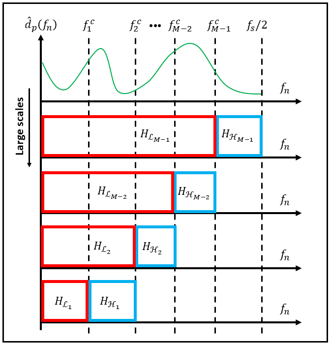
which are now guaranteed to be orthogonal. Finally, the spatial modes (the left singular vectors) are obtained as $\mathbf{L}=\mathbf{K}\,\mathbf{R}\,\mathbf{D}_{s^{2}}^{-1/2}$ , cf., Eq. 5.

The interested reader will find additional details on the mPOD method (e.g., how the filter bank is prepared) in the seminal publication [13]. One interesting property of the mPOD method is how the filter bank configuration defines the hierarchy of the scales resolved, Fig. 4 illustrates this point. The relationship of the mPODwith the DMD and RA methods is also covered in Ref. [13].

2.5.2 Multi-Resolution Dynamic Mode Decomposition

Multi-resolution strategies can also be combined with the Dynamic Mode Decomposition method: Kutz et al., in Ref. [14], proposed a reformulation of the classical DMD method capable of segregating the data into a hierarchy of multiresolution time-scale components resembling that given in Eq. (28). This reformulation, which is known as multi-resolution DMD (or mrDMD), operates as indicated in Fig. 5: if $n_{L}$ levels are to be considered, the classical DMD method of § 2.2 is applied $n_{b}\equiv 2^{n_{L}-1}$ times to the recursively halved dataset (i.e., of length $n_{t}/2^{l}$ ), with $l=0,\ldots,n_{L}-1$ . At each level, only the $r_{l}$ slowest (according to a user-specified threshold) modes are retained. The effect of this process is to recast Eq. (13) as:

\displaystyle\mathbf{v}(t_{j})=\sum_{i=1}^{r}\alpha_{i}\,\boldsymbol{\phi}_{i}\mu_{i}^{j\,\Delta\,t^{s}}=\sum_{l=1}^{n_{L}}\sum_{k=1}^{n_{b}}\sum_{i=1}^{r_{l}}\gamma^{l,k}\alpha_{i}^{l,k}\boldsymbol{\phi}_{i}^{l,k}(\mu_{i}^{l,k})^{j\,\Delta\,t^{s}},

(30)

where $n_{b}$ and $r_{l}$ are respectively the number of bins and the number of DMD modes retained at level $l$ , and $\gamma^{l,k}$ is an indicator function which equals $1$ if $t\in\left[t_{k},\,t_{k+1}\right]$ and $0$ elsewhere.

2.6 Resolvent Analysis

Let us now consider a linear(ized) dynamical system in continuous time subject to an external forcing:

\dot{\mathbf{v}}=\mathcal{A}^{c}\,\mathbf{v}+\mathbf{f}.

(31)

In equation above, $\mathcal{A}^{c}$ is the Jacobian matrix of the system, and the state $\mathbf{v}$ may represent fluctuations about a statistically stationary state; non–linearities can be included into the external forcing $\mathbf{f}$ .

It is well-known that the response of the system to harmonic excitations $\mathbf{f}=\hat{\mathbf{f}}e^{-i\,\omega\,t}$ is, invoking the linearity of the system (see e.g. Ref. [76]):

\hat{\mathbf{v}}=\underbrace{(-{i\mkern 1.0mu}\,\omega\mathbf{I}-\mathcal{A}^{c})^{-1}}_{\mathbf{H}(\omega)}\,\hat{\mathbf{f}}.

(32)

The spectral properties of the Resolvent operator $\mathbf{H}(\omega)$ defined above controls the ultimate fate of $\mathbf{v}$ , see e.g. Ref. [77]. Resolvent Analysis (RA) techniques are covered in Ref. [52], including an interpretation of Eq. (31) as the state–transition equation in a state–space representation of the system (i.e., input–output analysis, see also Refs. [77, 52]). Additionally, Towne et al. reveal in Ref. [11] the connections between the SPOD algorithm and RA techniques. However, and for brevity, in this work we focus exclusively on the data–driven formulation of the Resolvent Analysis (RA) technique recently proposed by Herrmann et al. in Ref. [43], which we discuss briefly next.

The data–driven Resolvent Analysis in Ref. [43] resorts to the exact DMD algorithm [78]. More specifically, if a certain weight matrix $\mathbf{W}$ is considered, first the transformed data sequence $\mathbf{U}_{1}^{n_{t}}=\mathbf{Q}\,\mathbf{V}_{1}^{n_{t}}$ is built; $\mathbf{Q}$ is the Cholesky factor of the weight matrix, namely $\mathbf{W}=\mathbf{Q}^{T}\,\mathbf{Q}$ . Then, partial subsequences $\mathbf{X}\equiv\mathbf{U}_{1}^{n_{t}-1}$ and $\mathbf{Y}\equiv\mathbf{U}_{2}^{n_{t}}$ are related through a variant of Eq. (9) (see also Ref. [64]), i.e.:

\displaystyle\mathbf{Y}=\underbrace{exp\left(\mathcal{A}^{c}\,\Delta t^{s}\right)}_{\mathbf{B}}\;\mathbf{X}.

(33)

Considering then a $r^{\prime}$ -rank SVD–reduced matrix $\bar{\mathbf{B}}$ , its eigenvalues $\boldsymbol{\Lambda}_{\bar{B}}$ and direct ( $\boldsymbol{\Psi}_{\bar{B}}$ ) and adjoint ( $\boldsymbol{\Psi}_{\bar{B}}^{\dagger}$ ) eigenvectors are computed. From them, an intermediate matrix and its QR decomposition: $\boldsymbol{\Psi}_{\bar{B}}^{H}\;\mathbf{W}\;\boldsymbol{\Psi}_{\bar{B}}\overset{\textbf{QR}}{=}\widetilde{\mathbf{F}}^{H}\widetilde{\mathbf{F}}$ leads to the approximated resolvent operator:

\displaystyle\widetilde{\mathbf{F}}\;\left(-\omega\,\mathbf{I}-\boldsymbol{\Lambda}_{\bar{B}}\right)\overset{\textbf{SVD}}{=}\mathbf{L}_{\bar{B}}\;\mathbf{S}_{\bar{B}}\;\mathbf{R}_{\bar{B}}^{H}.

(34)

whose complex SVD allows to obtain the forcing modes as:

\displaystyle\boldsymbol{\Phi}=\boldsymbol{\Psi}_{\bar{B}}\;\widetilde{\mathbf{F}}^{-1}\;\mathbf{R}_{\bar{B}},

(35)

whereas the response modes are given by:

\displaystyle\boldsymbol{\Psi}=\boldsymbol{\Psi}_{\bar{B}}\;\widetilde{\mathbf{F}}^{-1}\;\mathbf{L}_{\bar{B}}.

(36)

3 Numerical databases

In this work we aim at evaluating the performance of several publicly available data–driven, modal decomposition feature identification strategies. In an attempt to conduct an informative as possible comparison we will consider three different, increasingly complex flow datasets. The datasets chosen, which are also publicly available, are representative of three distinct flow regimes: laminar, turbulent and transitional.

The first testcase considered (which we term TC1) is the incompressible flow field around the mid-section of a very long cylinder. The flow dynamics of a relatively low Reynolds flow past a circular cylinder is well known, and has been studied in detail by Barkley & Henderson [79], among others. It is known that the flow bifurcation process in the wake of a circular cylinder starts at $\mathrm{Re}_{D}\simeq 48$ , where a Hopf bifurcation triggers the flow transition from symmetric, steady flow to unsteady two-dimensional flow [80]. Specifically, we consider a $\mathrm{Re}_{D}=U\,D/\nu=100$ flow, with $U$ the free stream velocity, $\nu$ the kinematic viscosity and $D$ the diameter of the cylinder. At these conditions the flow is laminar and two-dimensional. The flow shows a periodic vortex shedding with leading non-dimensional frequency Strouhal number $\mathrm{St}=f\,D/U=0.16$ , with $f$ the frequency in Hertz. All in all, this dataset is an ideal testcase to evaluate the performance of the methods considered herein.

The database employed is taken from Ref. [49]. The characteristics of this dataset (size per snapshot $n_{p}$ , number of snapshots $n_{t}$ , sampling period $\Delta\,t^{s}$ , most representative Strouhal, …) is summarized in Table 2. Figure 6 shows two representative snapshots of the stramwise velocity component in the database analysed. The figure also shows the temporal evolution of the streamwise and normal velocity components in a tracer point located at the wake: the periodic character of the velocity is evident.

The second testcase (TC2), originally described in Ref. [11], considers the pressure field in a turbulent jet flow. Although it is notorious that, in contrast to wall bounded turbulent flow [35], the frequency spectrum in jet flows presents selected high-amplitude frequencies, which are in charge of driving the flow dynamics. These high-amplitude frequencies are in many cases connected with flow instabilities occurring in the shear layer of the jet, which is in good agreement with the own nature of this type of flows.

Specifically, testcase TC2 is a turbulent jet at $\mathrm{Re}_{D}=\rho_{j}\,U_{j}\,D/\mu_{j}\approx 10^{6}$ , Mach number $\mathrm{M}=U_{j}/c_{j}=0.4$ and $T_{j}/T_{\infty}=1$ . Here $U$ is the velocity, $c$ is the speed of sound, $T$ is the temperature, $\rho$ is the density, D is the nozzle diameter, $\mu$ is the dynamic viscosity; the subscripts $j$ and $\infty$ refer respectively to the mean conditions at the nozzle exit and at the far field. At the present flow conditions, the flow is characterized by a high-amplitude frequency driving the flow dynamics at $\mathrm{St}\simeq 0.6$ (more details about this flow characterization in Ref. [11]). The high complexity and the turbulent character of this database is illustrated in Fig. 7: differences with Fig. 6) are striking, specially evident for the pressure signal behaviour.

This dataset has been derived from a Large Eddy Simulation computation, and hence contains a wide range of spatio-temporal scales interacting in complex manners. The dataset thus poses a challenge to the data analysis methods considered in this work. As before, the characteristics of this dataset are summarized in Table 2.

The third testcase (TC3) considers yet another incompressible laminar cylinder flow, but this time at $\mathrm{Re}_{D}=280$ , which is significantly more complex than TC1. As established above, beyond the first bifurcation at $\mathrm{Re}_{D}\simeq 48$ , the wake after the circular cylinder becomes unsteady, but the flow remains two–dimensional. If $\mathrm{Re}_{D}$ is further increased, a second flow bifurcation emerges at $\mathrm{Re}_{D}\simeq 190$ , and the bidimensional flow evolves into a three-dimensional flow [79]. Depending on the spanwise length of the cylinder, defined as $L_{z}=2\pi/\beta$ with $\beta$ the spanwise wavenumber, differences are found on the value for the critical Reynolds number and the system dynamics [81].

In this work, we consider $L_{z}=6.99$ , which corresponds to a periodic flow, where a three-dimensional instability is leading the flow changes driven by a mode with critical wavenumber $\beta\simeq 7.570$ (more details in Ref. [73]). Thus, at the present flow condition (i.e. $\mathrm{Re}_{D}=280$ , $L_{z}=6.99$ ), the stationary solution is periodic, with leading frequency $\mathrm{St}=0.21$ . In the transient regime of the simulation, frequency $\mathrm{St}=0.36$ is also identified with high amplitude but negative growth rate, as we shall discuss below. The latter frequency is connected to the transition to a three–dimensional quasi–periodic flow, which is a flow bifurcation that takes place at $\mathrm{Re}_{D}\simeq 380$ , see Blackburn et al. [81]. Note that this second high-amplitude frequency disappears when the analysis is carried out in the saturated flow (i.e., when the stationary state is reached).

Dataset TC3, available from Ref. [57], contains unsteady three-dimensional flow data (see Fig. 8). The database includes snapshots collected since the beginning of the numerical simulation, which allows to assess the performance of the data–driven methods also for transient solutions, thus revealing the capabilities and limitations of these tools when predicting the leading dynamics of the flow. In other words, TC3 illustrates the performance of the methods as predictive reduced order models. If the dynamics are properly identified in transient solutions, then it is possible to reduce the computational cost of numerical simulations, which could be suitable for future flow control applications. As before, the characteristics of the database are summarized in Table 2.

Table 2: Summary of the main characteristics of the three testcases.

n_{p}

and

n_{t}

represent the dimensions of the snapshot matrix (Eq. (1)) on the

X

and

Y

axis, respectively and

\Delta t^{s}

represent the sampling rate.

Testcase $[x_{min},x_{max}]\times[y_{min},y_{max}]\times[z_{min},z_{max}]$ $n_{x}\times n_{y}\times n_{z}$ Variables $n_{p}$ $n_{t}$ $\Delta t^{s}$ Target $\mathrm{St}$ TC1 (laminar, 2D) $[-1,9]\times[0,2]$ $449\times 199$ $(u_{x},u_{y})$ $1.78\times 10^{5}$ $151$ $0.2$ $0.16$ TC2 (turbulent, axisymmetric) $[0,20]\times[0,4]$ $39\times 175$ $p$ $6.83\times 10^{3}$ $5000$ $0.2$ $0.6$ TC3 (transitional, 3D) $[0,10]\times[-2,2]\times[0,6.99]$ $100\times 40\times 64$ $(u_{x},u_{y},u_{z})$ $7.68\times 10^{5}$ $599$ $1$ $0.21$ ( $0.36$ )

4 Method comparison

Section § 2 has described in, hopefully, sufficient detail the different methods considered. In This section we offers an additional comparison where we investigate whether the different techniques considered are capable of identifying the most relevant frequencies: $St\approx 0.16$ for TC1, $St\approx 0.6$ for TC2 and $St\approx 0.21$ and $St\approx 0.36$ for TC3, as the quality of the dataset is worsened by shortening (i.e., by discarding an increasing number of the latter temporal samples of the dataset). This test assesses how good the different techniques are in extracting meaningful information from partial data.

The results of the aforementioned evaluation are presented on a testcases basis. We start by considering the results for TC1, as can be seen in Fig. 9a, DMD and DMD-based methods functions very well in identifying the dominant frequency, even when the data is limited (shortened). However, if we take a look to Fig. 9b, we can see that FFT and POD-based techniques perform poorly when compared with DMD-based methods. If we consider FFT as an example, we can see that this technique only identifies the right frequencies when the number of snapshots taken is a multiple of 30, otherwise the technique is experiencing what is called "spectral leaking", which is the same case as POD, SPOD or mPOD. Hence these techniques may perform sub-optimally in cases sparse data, unlike DMD based approaches. Also, to obtain similar results, FFT requires a longer data sequence than the other methods, which can be a disadvantage for large databases. However, FFT is a robust method that always identifies the relevant dynamics, even when the spectral complexity is much larger as the spatial complexity, which is a common case in the performance of experimental sensor measurements. In TC2, The dataset describes a complex, turbulent pressure field. As it is usual in turbulent flows, a large number of temporal samples is necessary to provide a good representation of the underlying physical process. In this manner, the initial number of samples ( $n^{\prime}_{t}=5000$ ) justifies why the results provided by the different methods are reasonably good, as we can see in Figures 10a and 10b. The large number of spatio-temporal scales driving the dynamics of turbulent flows, makes it challenging to identify the most relevant dynamics. However, the present test case studied the main changes in the flow are driven by a strong global flow instability, that all the methods are capable to identify. The definition of the rest of the dynamics varies depending of the method used, consequently varying the reconstruction error of the main database. In TC3, the methods are capable to capture the main dynamics, even in the transient regime. Similarly to TC2, the flow instabilities are well defined. The method differences are found in the accuracy of the main frequencies captured and the reconstruction of the main dynamics. (as shown in Figures 11a and 11b).
Hence, regarding the achievement of the main goal, which is capturing the dominant frequencies: $St\approx 0.16$ for TC1, $St\approx 0.6$ for TC2 and $St\approx 0.21$ and $St\approx 0.36$ for TC3, all the methods were successful, especially in TC1. In the more complex cases, as in TC2 and TC3, we can notice a small fluctuation in the frequencies depending on the number of snapshots, where some methods may suffer spectral leaking and others may identify several frequencies with comparable amplitude levels. However, these results are considered reasonable because of the flow complexity, which is larger in the turbulent and transient flow. Consequently, the methods are expected to face difficulties in identifying the dominant dynamics and avoiding the components related to the small flow scales of the transient regime. Nevertheless, all the methods eventually converge and we can highlight the fact that the HODMD algorithm is the fastest to converge in all testcases.

In the following of the paper, we will try to understand the performance of all the methods studying carefully each one of the testcases.

5 Results

In this section we discuss the results obtained when applying the different data–driven modal decomposition methods to the datasets TC1–TC3. We follow the structure laid out in section 2, and begin with the results obtained with the most classical methods (POD, DMD and FFT), and continue with the improved methods that employ data redundacy (SPOD and HODMD). We follow next with multi–resolution methods (mPOD and mrDMD), and finish with data–driven resolvent analysis (RA).

All the computations have been performed on a desktop computer equipped with a $4$ -core Intel $(R)$ Core $(TM)$ i5-3570K CPU at $3.40\,GHz$ , a cache memory of $6144\,kB$ and $8.0\,GB$ of RAM.

5.1 Feature detection using classical methods: POD, DMD and FFT

This section describes the results obtained through application of the most established methods, namely POD, DMD and FFT to the datasets TC1-TC3. Figure 12-left shows the singular values obtained when POD is applied to analyse TC1, the two-dimensional cylinder wake. Observe how, the singular values are grouped in pairs of frequencies, which is a reflection of the strong periodic character of the flow [82]. Fig. 12-right shows the amplitudes of the DMD modes as function of frequency $\mathrm{St}$ , which, by a certain abuse of language, is usually termed DMD spectrum. The spectrum shows that the most relevant mode appears at the leading frequency $\mathrm{St}\approx 0.16$ ; $7$ distinctly large amplitudes also appear at integer multiples of the leading frequency: these are harmonics of the leading mode. Note that in the stationary regime, the growth rates $Re(\lambda)$ , should be zero. In noisy databases (or numerical simulations that still are not saturated in time), the growth rates are never exactly zero, since the value they take is of the same order of magnitude as the level of noise. This in turn provides an estimation of the error made in the frequency calculations (see more details in Refs. [83, 34, 74]).

Fig. 13 shows the mean flow and the most relevant POD/DMD modes. Note how the mean flow and the DMD mode at $\mathrm{St}=0$ are similar, suggesting that the steady DMD mode represents the mean flow, see Ref. [73]. Regarding the remaining modes, observe how these modes are qualitatively similar. Recall that (Sec 2) POD modes are real, whereas DMD modes appear in complex conjugate pairs; note also how the real and imaginary part of the DMD modes are phase shifted, revealing the travelling character of the modes in the wake flow.

However, note that TC1 is a dataset describing a two-dimensional, laminar, coherent and well organized motion (the wake) generated by a highly accurate numerical solver (i.e., relatively clean from noise): it should not be surprising that POD and DMD analyses provide comparable results. For example, Fig. 14 shows the frequency content of the first three dominant POD modes (calculated using FFT on the corresponding temporal POD mode $\mathbf{r}_{0,j}$ , Eq. (3)). This behaviour is tipically observed whenever both DMD and POD are applied to analyse transient data from linear solutions. In those cases, POD, DMD, but also linear global stability modes are the same (see details and more results in Ref. [84]).

In fluid dynamic applications, this SVD-enabled reduction is useful at two levels: on the one hand, since most datasets are densely discretized in space and sampled frequently in time (i.e., they are large); SVD helps to reduce the memory footprint of the DMD analysis. On the other hand, the optimal representation properties of SVD become useful to filter noise and spatial redundancies, i.e. to clean the data. At each SVD step^§^§ § There is one SVD step for classical DMD, and two for HODMD, section 2, the rank of the scaled chronos matrix $\mathcal{C}_{1}^{n_{t}-1}$ (Eq. (25)) can be controlled directly (setting $r^{\prime}$ ) or indirectly (via the tolerance $\varepsilon_{1}$ , Sec. 2.4.2). Usually, larger tolerances (i.e., more SVD modes retained) help the method to properly identify the main dynamics of the system. However, and somewhat contradictorily, complex flows datasets (i.e., multi-scale, turbulence, noise, etc.) ask for as intense dimensionality reductions as possible. The user needs thus to perform this reduction carefully, as suboptimal $\varepsilon_{1}$ values can lead even to failure of the method. This behaviour is connected to the spectral and spatial complexities introduced in sections 2.2 and 2.4.2. Similarly, the DMD frequency spectrum is also sensitive to the number of grid points composing the spatial domain. For instance, in experimental measurements, if the number of spatial points (spatial complexity) is smaller than the spectral complexity (number of frequencies retained in the DMD expansion Eq. (30)), then DMD fails. In such cases, other methods, like POD, FFT, or the more robust approaches SPOD and HODMD arise as sensible alternatives.

We present now the FFT results. Fig. 15-top shows the Fourier spectrum calculated for TC1, computed using Eq. (17). Observe how for this simple, strongly periodic flow, FFT identifies the same frequencies as POD and DMD. Fig. 15b shows the spatial distribution of the horizontal component of the FFT mode at $\mathrm{St}\approx 0.16$ , This information reveals that most energetic areas lie in the wake of the cylinder. According to the horizontal component, relevant information lies symmetrically above and below the $y=0$ line. The spatial information provided by the FFT method is not as easily interpretable as that provided by the POD/DMD methods. However, this is easy to anticipate, if one recalls that FFT operates on the temporal correlation matrix (see Sections 2.3 and 2.5), which means that spatial information is given up to a certain extent.

As we have observed so far, classical data–driven modal decomposition methods, namely POD, DMD and FFT provide comparable results whenever they are applied to flow databases describing a strongly coherent behaviour. We investigate now how these techniques perform when confronted with more complicated flows, namely the fully turbulent jet flow (TC2) and the transitional, three-dimensional cylinder flow (TC3) databases. In this last case, we consider two differentiated temporal ranges, which we respectively term transient regime $\left(t\in[300,\,420]\right)$ and saturated regime $\left(t\in[450,\,570]\right)$ , see Fig. 8-right.

Concerning TC2, Figure 16-left presents the singular values obtained with POD. Observe the radical difference in the decay rate of the singular values for TC2 with respect to the more simple TC1: whereas for TC1 (Fig. 12-left) the $s_{i}$ ’s (Eq. (3)) decay relatively fast and stabilize at around $10^{-6}$ , the $s_{i}$ ’s for TC2 decay also very fast at first, and slightly slower afterwards; however, there is not an index $i$ beyond which the singular values become negligible, or even stabilize. This behaviour is consistent with the multiscale nature of turbulence: in a turbulent flow, all the scales contribute with energy.

Figure 16-right shows the DMD spectrum: observe how relevant modes appear to be the steady component and that at $\mathrm{St}\approx 0.6$ and $St\approx 0.43$ . However, several DMD modes present amplitudes at relatively high levels, some of them comparable to the mode at $\mathrm{St}\approx 0.6$ . And in this case it is much more difficult to establish a clear amplitude-based criterion to consider or not a specific DMD mode. In this turbulent case, the overall picture is not as clear as it was for TC1.

Fig. 17 shows the mean flow and the most relevant POD/DMD modes. Again we observe the coincidence in shape of the mean flow and the DMD mode at $\mathrm{St}=0$ . Both the real POD modes and the complex DMD modes present features reminiscent of coherent wavepacket structures [11].

Fig. 18 presents the frequency content of the first three dominant POD modes. The spectral content of the POD modes is not as clean as those from TC1; rather, for each POD mode, all the frequencies are active, which is to be expected in a complex, turbulent flow. It is worth mentioning that the dominant frequencies obtained through the spectrum in Fig. 18 coincide with the dominant frequencies of DMD, Fig. 16-right. On the other hand, DMD is conceived so that DMD modes are associated with distinct, individual frequencies. However, that is of little help in this case, recall the amplitudes vs non-dimensional frequencies distribution in Fig. 16. The situation is not better for the FFT analysis, see Fig. 19. In conclusion, as soon as datasets with certain complexity, data analysis tools with better performance become necessary.

As for TC3, Figure 20-left presents the singular values obtained by POD applied to the $z$ -component of the velocity. The singular value distributions are closer to that in TC1 than that in TC2; in fact, singular values could be grouped in pairs again. Note how, beyond the index $10$ , the energy of the POD modes is comparatively larger in the transient regime, as there are several flow structures that have not yet attenuated. The DMD spectrum is also much simpler, and the modes at $\mathrm{St}\approx 0.21$ and $0.36$ are easily identified. This apparent simplicity is again a reflection of the laminarity of the dataset. However, TC3 is more complex than TC1, and this is observed in the spatial support of the POD/DMD modes shown in Fig. 21. The spanwise modulation of the modes is consistent with that of the flow solution, see Fig. 8.

Fig. 22 presents the frequency content of the first three dominant POD modes. Again, the spectral content of the POD modes is relatively simple; however, a single, distinct frequency cannot be assigned to each mode, as expected. In fact, the second POD mode is linked to a frequency approximately double of $\mathrm{St}\approx 0.21$ , but a trace of $\mathrm{St}\approx 0.36$ is also visible; the third POD mode is linked to $\mathrm{St}\approx 0.36$ and yet is also contaminated by the first harmonic.

The FFT analysis is summarized in Fig. 23. The spectrum at a tracer point reveals the components at $\mathrm{St}\approx 0.21$ and $\mathrm{St}\approx 0.36$ , but contributions at other frequencies are also appreciable. The spatial distribution of the horizontal FFT mode at $\mathrm{St}\approx 0.21$ is different from that shown in Fig. 15, e.g., it is slightly asymmetric. The spanwise modulation is specially visible in the FFT mode at $\mathrm{St}\approx 0.21$ obtained from transversal velocity component of the dataset, Fig. 23-bottom.

5.2 Improving accuracy through redundancy: SPOD and HODMD

We discuss now the results of the analysis using SPOD and HODMD methods to the datasets TC1-TC3.

Figures 24 and 25 present the SPOD (top) and HODMD (bottom) spectra. In particular, we investigate the influence of the window length (given by $n_{t}^{\prime}$ for SPOD and $d$ for HODMD) on the results obtained for TC1. In a first comparison, we set window lengths that are powers of $2$ , in order to obtain the optimal performance of the underlying FFT algorithm. Regarding the SPOD spectrum (Fig. 24-top, obtained with an overlap of $50\%$ and the Hamming window function), the first SPOD mode is most energetic at $\mathrm{St}\in\left(0.15,0.25\right)$ , depending on the choice of the parameters. This is a sign of spectral leaking [56], derived from the relatively short temporal sequence. Regarding the HODMD results, Fig. 24 shows the sensitivity of the HODMD spectrum to window length (bottom left) and the tolerance in Eq. 7: the higher the value, the less modes are retained in the reconstruction, and hence the fewer modes identified.

SPOD retrieves the correct frequencies if window lengths multiple of $15$ are employed, as these leads to a set of bins coinciding with $\mathrm{St}\approx 0.16$ . These results are also summarized in Fig. 25. The HODMD results appear also in Fig. 25. The SPOD and HODMD modes are shown in Fig. 26 and Fig. 27. They look very similar to those obtained by POD and DMD.

The spectra for the turbulent jet dataset (TC2) are summarized in Fig. 28. This dataset is much longer ( $n_{t}=5000$ ), which allows for more flexibility in the choice of the SPOD window length $n_{t}^{\prime}$ ; again we consider powers of $2$ . Fig. 28 (top) confirms that the most energetic SPOD mode is most active at $\mathrm{St}\approx 0.6$ . Fig. 29 (bottom) shows the largest amplitude HODMD modes and its sensitivity to $d$ and $\varepsilon_{1}=\varepsilon_{2}$ . In this case, the modes retrieved cover a range of $\alpha_{i}/\alpha_{max}\in\left(0.5,1\right)$ . For values of $d=128-256$ and $\varepsilon_{1}=\varepsilon_{2}\in\left(0.2,0.3\right)$ , the most relevant mode appears at the expected $\mathrm{St}\approx 0.6$ . The spatial support of both the SPOD and HODMD modes is shown in Fig. 29, which again are very similar to those obtained by POD and DMD.

Regarding the three-dimensional laminar cylinder flow (TC3), the study is conducted on sections of the dataset of $n_{t}=120$ , following [57]. In this case, the target frequency is mainly $\mathrm{St}\approx 0.21$ and $\mathrm{St}\approx 0.36$ , and thus we will consider window lengths up to $64$ snapshots, so that the resulting bins can capture that frequency. Fig. 30 (top) shows the most energetic SPOD mode. For a window length $n_{t}^{\prime}=64$ , this mode has largest energy at $\mathrm{St}\approx 0.21$ , also $\mathrm{St}\approx 0.36$ seems to be relevant. For window lengths $n_{t}^{\prime}=16$ and $32$ , the bin resolution is not enough for singling out the frequency of interest. Fig. 31 (bottom) shows again the largest amplitude HODMD modes and its sensitivity to $d$ and $\varepsilon_{1}=\varepsilon_{2}$ . In this case, the modes retrieved cover a range of $\alpha_{i}/\alpha_{max}\in\left(10^{-3},1\right)$ ; the most relevant modes appear at the frequencies $\mathrm{St}\approx 0.21$ and $0.36$ . The spatial support of both the SPOD and HODMD modes is shown in Fig. 31, which again are very similar to those obtained by POD and DMD.
The advantages of using SPOD and HODMD in complex flows compared to classical POD, DMD or FFT is clear. Both SPOD and HODMD offer cleaner and more accurate results that their standard counterparts. This is very useful to develop ROMs, capable to reconstruct the original datasets and suitable for data forecasting (see Refs. [74, 60, 72]). Finally, as we investigated the performance of these two methods on both, saturated (see Figures 30 and 31) and transient regimes (results are not included for their similarity to the saturated case, as well as for brevity) of TC3. We can conclude that the advantage of HODMD is in the two tolerances of the algorithm, which are capable to reduce the data dimensionality, to remove spatial redundancies, and then to retain the most relevant spectral modes, as well as the luck of spectral leakage which is caused by DFT in SPOD.

5.3 Feature detection based on multi-resolution analyses: mPOD and mrDMD

The multi-resolution techniques mPOD and mrDMD, extensions of POD and DMD respectively, are suitable to identify different spatio-temporal scales defining the flow dynamics. Their application should be carried out in complex flows. The window size and the frequency filter selected in both methodologies is crucial to be able to progressively differentiate fast and low frequencies, properly modelling the flow physics. These methods, and specially mrDMD, require a careful calibration, with the aim at obtaining robust results, and to be capable to differentiate the fast physical frequencies from unrealistic fast frequencies, which are erroneously captured by the method mixing chaotic dynamics with the periodic or quasi-periodic physical modes driving the flow.

Figures 32 and 33 show the three most energetic mPOD modes and their corresponding frequencies for all three testcases, as well as filter banks $\left(f_{c}\right)$ . It is worth mentioning that in order to choose a suitable filter bank, prior knowledge about the flow is necessary.

However, in the mPOD case, to properly identify the main flow dynamics, and to differentiate spurious from physical modes, it is necessary to have a prior knowledge of the frequencies driving the flow. In this way, it is possible to establish a proper low-pass or high-pass filter frequency band, which is a part of the methodology.

Using multi-resolution analyses is recommendable when the user wants to identify specific frequencies from a highly complex spatio-temporal flow. These methods will be then able to differentiate fast and low events, representing physical solutions, or connected to specific noise or input (or external known) signals that for some specific reasons, it is worth to know with detail to characterize the flow.

The mrDMD spectra are shown in Fig. 34. For TC1 and TC3 it is easy to identify dominant frequency but for TC2 we have several ranges of dominant frequency. The advantage of mrDMD is that we have information not only in frequency but also in time. Although we need to have prior knowledge of flow dynamics in order to calibrate mrDMD hyper-parameters.

The spatial modes of all testcases are visually indistinguishable of those shown in Figures 13, 17, 21, and -for the sake of brevity- are not shown here.

5.4 Beyond classical applications: resolvent analysis

In this section we explore the performance of the data-driven implementation of the Resolvent Analysis RA on the three testcases investigated in this work.

Figure. 35 shows how the RA technique is capturing the frequencies in all testcases. Regarding TC1, and as can be seen in the Fig. 35a, the RA was capable of capturing the wanted frequency (0.16), but not as the dominant frequency, as it identified two other harmonics as dominant frequencies. We can notice similar behavior in TC2 as well, where RA captures the relevant frequencies, but it also gave more importance to the smaller frequencies (see Fig. 35b), and more accurate results can be obtained only when the frequencies are re-scaled (through the multiplication by $St$ ) as shown in Fig. 35c. Same comments can also be applied to the results of TC3. Once again, the relevant frequencies are captured in both, the transient regime (Fig. 35d) and saturated regime (Fig. 35e), but other harmonics are also captured as dominant frequencies.

Figure. 36 represents the modes obtained by the RA when applied to TC1, TC2 and TC3. In the case of TC1, as we can see in Fig. 36a the forcing and response modes are similar, and that is because the flow is saturated. Meanwhile in TC2, the growth rates are continuously changing, which will lead the difference between the forcing and response modes as seen in Fig. 36b, however the response mode is similar to the DMD and POD modes.

Regarding TC3, we have applied the RA on the saturated regime, where the growth rates are also changing, hence, the forcing and response modes are different as seen in Fig. 36c, but again, the response mode is similar to the DMD mode. In this testcase in particular, we apply the RA algorithm to calculate the forcing needed to obtain the response of the DMD mode in a system.

6 Conclusions

In this work, we compare eight different modal decomposition techniques with the aim at introducing a critical assessment on what are the main benefits and constrains of each method as function of their application. This comparison involves three classical methods: Fast Fourier Transform (FFT), Proper Orthogonal Decomposition (POD) and Dynamic Mode Decomposition (DMD), four extensions of the classical methods: Spectral POD (SPOD), multi-scale POD (mPOD), Higher Order DMD (HODMD) and multi-resolution DMD (mrDMD) and finally, the Resolvent Analysis (RA). To the best of the authors’ knowledge, this is the first time a review paper have gathered and compared all these modal decomposition techniques.

In order to provide an as fair as possible comparison, all the techniques have been applied to three testcases. The testcases are coded as TC1, TC2 and TC3 and they are ordered with respect to their level of complexity. The first testcase considered was the velocity field of the laminar wake around cylinder at $Re_{D}=100$ , the second testcase is the pressure field of a turbulent jet flow at $Re_{D}=10^{6}$ and the third and final testcase is the velocity field of the three dimensional transient wake around cylinder at $Re_{D}=280$ . The first contribution in this work is a comparison between the performance of these methods in identifying the relevant frequencies when the databases are shortened. The obtained results imply the following: in cases where the data is limited, the DMD-based methods outperform FFT and POD-based methods. As DMD-based methods deliver accurate results, mostly regardless of the size of the dataset and the window length, meanwhile POD-based methods are tightened with some limitations as spectral leaking. Nevertheless, when taking larger amounts of data, all the methods deliver, in one way or another, comparable results. Furthermore, some of the methods fluctuate in frequencies based on the amount of data available, and this is linked to the flow complexity. As in these cases (TC2 and TC3), the methods are are exposed to failure in avoiding the modes connected to small flow scales.
Next,the performance of these algorithms is thoroughly assessed concerning both the accuracy of the results and how these algorithms function with limited amounts of data. The obtained results are as follow:
As for the classical methods, POD, DMD and FFT, all the methods were able to identify the dominant frequency as $\mathrm{St}\approx 0.16$ for TC1, but did not perform as good for TC2, as they all struggled in separating the relevant frequency at $\mathrm{St}\approx 0.6$ from other harmonics. For TC3, when DMD easily captured the main frequencies at $\mathrm{St}\approx 0.21$ and $\mathrm{St}\approx 0.36$ , both POD and FFT were facing some difficulties in identifying the exact frequencies. Concerning the extension of the classical methods We start with the results obtained from SPOD and HODMD. The results obtained by the HODMD algorithm were quite accurate and robust, as it was able to capture the relevant frequencies in all testcases. For SPOD, even though the techniques was able to capture the wanted frequencies, it was not an easy task. This technique, which usually deals with statistically stationary data, suffered from spectral leaking in all testcases. Regrading mPOD and mrDMD, both methods identified the main frequency in TC1 without any trouble. However, a slight error in the frequencies was noticed in TC2 and TC3. As for the modes obtained by all the previously mentioned methods, they were all visually indistinguishable and consistent with the ones of the flow solution.

Finally, the RA. When applying this technique to all testcases, the RA algorithm was able to capture the target frequencies, but not as dominant ones: there were always other modes that have been given more importance. Furthermore, the forcing and response modes are similar in TC1, because of the simplicity of the testcase, In the more complex testcases, the forcing and response mode are markedly different. Yet, the response modes are always similar to the modes obtained by the other techniques.

Acknowledgment

This work has been supported by SIMOPAIR (Project No. REF: RTI2018-097075-B-I00) funded by MCIN/AEI/10.13039/501100011033 and by the European Union’s Horizon 2020 research and innovation program under the Marie Skłodowska-Curie Agreement number 101019137— FLOWCID. S.L.C. acknowledges the grant PID2020-114173RB-I00 funded by MCIN/AEI/10.13039/501100011033. The authors also acknowledge the support provided by Grant TED2021-129774B-C21, funded by MCIN/AEI/10.13039/501100011033 and by the European Union "NextGenerationEU"/PRTR.

Appendix A On the DMD amplitudes

A.1 Computing the DMD amplitudes

Since the introduction of the DMD method, a variety of strategies have been proposed to discriminate the relative importance of the dynamic modes identified. One of the earliest approaches, applied in the context of companion-matrix DMD, simply compares the norm of the modes [62].

Other alternatives resort to the factorization model in Eq. (14); these approaches aim at identifying the amplitudes $\alpha_{i}$ . One strategy obtains the $\alpha_{i}$ by projecting the first snapshot over the DMD basis [49] through Moore-Penrose pseudoinversion, $\boldsymbol{\alpha}=\boldsymbol{\Phi}^{+}\,\mathbf{v}_{1}$ . Note that, since matrix $\mathbf{L}_{0}$ is unitary, this step can be also accomplished at a reduced computational cost using the reduced chronos matrix:

\displaystyle\boldsymbol{\alpha}=\boldsymbol{\Psi}^{+}\,\mathbf{c}_{1}.

(37)

Another alternative, rooted also on the factorization framework of Eq. (14), poses and solves a minimization problem in the Frobenius norm [55]:

\displaystyle\min\limits_{\alpha_{i}}\|\mathbf{V}_{1}^{n_{t}-1}-\boldsymbol{\Phi}\mathbf{D}_{\alpha}\mathbf{V}_{\mu}\|^{2}_{F},

(38)

Again, the fact that matrix $\mathbf{L}_{0}$ is unitary and does not affect the norm in Eq. 38, leads to the optimization problem:

\displaystyle\min\limits_{\alpha_{i}}\|\mathcal{C}_{1}^{n_{t}-1}-\boldsymbol{\Psi}\mathbf{D}_{\alpha}\mathbf{V}_{\mu}\|^{2}_{F}.

(39)

Figure 37 illustrates the concepts covered in the previous discussion using the TC1 dataset. Fig. 37a compares the relative importance of the DMD modes identified by both the companion and the similarity transformation based DMD algorithms, using either the companion DMD mode norms [62] or the amplitudes obtained using Eq. (39) [55]. In both cases, the frequency associated to the vortex shedding of the wake is clearly identified. Also, note how Fig. 37b confirms that both companion and the similarity transformation based DMD algorithms identify the same Ritz values. Finally, Fig. 37c illustrates the difference in amplitudes obtained by projecting simply on the first snapshot (Eq. (37)) or on the whole data matrix (Eq. (39)). Table 3 offers complementary information on the reconstruction error $\min\limits_{\alpha_{i}}\|\mathcal{C}_{1}^{n_{t}-1}-\boldsymbol{\Psi}\mathbf{D}_{\alpha}\mathbf{V}_{\mu}\|^{2}_{F}$ achieved and the computational effort required for each approach, averaged for three different realizations.

In view of this analysis, in this contribution we have favoured the approach given in Eq. (39) for the computation of the amplitudes.

Table 3: Two-dimensional laminar wake around cylinder at

\mathrm{Re}_{D}=100

: comparison of strategies to assess the relative importance of the different DMD modes, using different techniques.

Method	Reconstruction error	Computing time $[s]$
Companion DMD [62]	N.A.	$4.72\times 10^{-2}$
Eq. (37)	$1.64\times 10^{-6}$	$1.85$
Eq. (39)	$5.85\times 10^{-13}$	$6.53\times 10^{-4}$

A.2 Computing the HODMD amplitudes

The amplitudes identification in the HODMD method requires solving an overdetemined system of equations given by (see [34, 57]):

\displaystyle\mathbf{C}\,\boldsymbol{\alpha}=\mathbf{r},

(40)

where the coefficient matrix $\mathbf{C}$ is defined as:

\displaystyle\mathbf{C}=\begin{bmatrix}\boldsymbol{\Psi}^{\prime}\\ \boldsymbol{\Psi}^{\prime}\,\mathbf{D}_{\mu}\\ \vdots\\ \boldsymbol{\Psi}^{\prime}\,\mathbf{D}_{\mu}^{n_{t}-1}\end{bmatrix},

(41)

with $\mathbf{D}_{\mu}$ a diagonal matrix whose non-zero elements are the Ritz values $\mu_{i}$ . The forcing term $\mathbf{r}$ is given by:

\displaystyle\mathbf{r}=\begin{bmatrix}\mathbf{c}_{1}\\ \mathbf{c}_{2}\\ \vdots\\ \mathbf{c}_{n_{t}}\\ \end{bmatrix}.

(42)

This linear system is solved in the least-squares sense, which de facto implies solving:

\displaystyle\mathbf{C}^{H}\mathbf{C}\,\boldsymbol{\alpha}=\mathbf{C}^{H}\,\mathbf{r}.

(43)

This system is solved using pseudo-inversion based on SVD decomposition.

For certain large databases, the memory footprint for computing the pseudo-inverse of $\mathbf{C}$ can exceed the RAM available. In those cases, the structure of $\mathbf{C}$ can still be exploited to obtain $\boldsymbol{\alpha}$ . Indeed, matrix $\mathbf{C}^{H}\mathbf{C}$ can be recast as:

\displaystyle\mathbf{C}^{H}\mathbf{C}=\sum\limits_{k=1}^{n_{t}}(\mathbf{D}_{\mu}^{k-1})^{H}\boldsymbol{\Psi}^{\prime H}\,\boldsymbol{\Psi}^{\prime}\,\mathbf{D}_{\mu}^{k-1},

(44)

whereas the product $\mathbf{C}^{H}\mathbf{r}$ turns out to be:

\displaystyle\mathbf{C}^{H}\mathbf{r}=\sum\limits_{k=1}^{n_{t}}(\mathbf{D}_{\mu}^{k-1})^{H}\boldsymbol{\Psi}^{\prime H}\,\mathbf{c}_{k},

(45)

Fig. 38 shows the result of this alternative strategy for TC1 case, showing that both strategies give the same result.

A.3 Selecting the DMD amplitudes

In section 2 we discussed how, and differently from the eigenvalues obtained in POD-based modes (i.e., $s_{j}=\sqrt{\lambda_{j}}$ ), the DMD amplitudes do not have a direct interpretation as energies. This implies that DMD modes cannot be sorted rigourously according to moduli $\left|\alpha_{i}\right|$ : e.g., modes with large $\left|\alpha_{i}\right|$ might be decaying fast, i.e., have large decrease rate $\mathrm{Re}{(\lambda_{i})}\ll 0$ , or alternatively, modes with moderate $\left|\alpha_{i}\right|$ might be long lived ( $\mathrm{Re}{(\lambda_{i})}\approx 0$ ) or even unstable ( $\mathrm{Re}{(\lambda_{i})}>0$ ).

Several criteria have been derived to recognize such situations, see e.g. [85, 86]. In this work, we consider the criterion proposed in [87] to investigate transition in turbulent channels. The criterion sorts modes according to the following quantity:

\gamma_{i}=|\alpha_{i}|\;\frac{e^{\mathrm{Re}(\lambda_{i})\Delta t}-1}{\mathrm{Re}(\lambda_{i})}.

(46)

This criterion has been applied to the dataset TC3, for both the transient and saturated regimes. Fig. 40

References

[1] L. Sirovich, Turbulence and the dynamics of coherent structures. I. coherent structures, Q. Appl. Math. 45 (3) (1987) 561–571.
[2] L. Sirovich, M. Kirby, Low-dimensional procedure for the characterization of human faces, Josa a 4 (3) (1987) 519–524.
[3] C. Tropea, A. L. Yarin, J. F. Foss, et al., Springer handbook of experimental fluid mechanics, Vol. 1, Springer, 2007.
[4] J. Borée, Extended proper orthogonal decomposition: a tool to analyse correlated events in turbulent flows, Experiments in fluids 35 (2) (2003) 188–192.
[5] A. V. Cavalieri, A. F. da Silva, Cross proper orthogonal decomposition, Physical Review Fluids 6 (1) (2021) 014602.
[6] M. O. Williams, I. G. Kevrekidis, C. W. Rowley, A data–driven approximation of the koopman operator: Extending dynamic mode decomposition, Journal of Nonlinear Science 25 (6) (2015) 1307–1346.
[7] M. R. Jovanović, P. J. Schmid, J. W. Nichols, Sparsity-promoting dynamic mode decomposition, Physics of Fluids 26 (2) (2014) 024103.
[8] J. L. Proctor, S. L. Brunton, J. N. Kutz, Dynamic mode decomposition with control, SIAM Journal on Applied Dynamical Systems 15 (1) (2016) 142–161.
[9] P. Schmid, J. Sesterhenn, Dynamic mode decomposition of numerical and experimental data, J. Fluid Mech. 656 (11 2008). doi:10.1017/S0022112010001217.
[10] J. W. Cooley, J. W. Tukey, An algorithm for the machine calculation of complex Fourier series, Math. Comput. 19 (2) (1965) 297–301. arXiv:https://doi.org/10.1137/15M1054924, doi:10.1090/S0025-5718-1965-0178586-1.
URL https://doi.org/10.1090/S0025-5718-1965-0178586-1
[11] A. Towne, O. Schmidt, T. Colonius, Spectral proper orthogonal decomposition and its relationship to dynamic mode decomposition and resolvent analysis, J. Fluid Mech. 847 (2018) 821–867. doi:10.1017/jfm.2018.283.
[12] S. Le Clainche, J. M. Vega, Higher Order Dynamic Mode Decomposition, SIAM J. Appl. Dyn. Syst. 16 (2) (2017) 882–925. arXiv:https://doi.org/10.1137/15M1054924, doi:10.1137/15M1054924.
URL https://doi.org/10.1137/15M1054924
[13] M. A. Mendez, M. Balabane, J.-M. Buchlin, Multi-scale proper orthogonal decomposition of complex fluid flows, J. Fluid Mech. 870 (2019) 988–1036. doi:10.1017/jfm.2019.212.
[14] J. N. Kutz, X. Fu, S. L. Brunton, Multi-resolution dynamic mode decomposition, SIAM J. Appl. Dyn. Syst. 15 (2) (2016) 713–735.
[15] M. R. Jovanović, B. Bamieh, Componentwise energy amplification in channel flows, J. Fluid Mech. 534 (2005) 145–183.
[16] J. L. Lumley, The structure of inhomogeneous turbulent flows, Atmospheric Turbulence and Radio Wave Propagation (1967) 166–177.
[17] J. L. Lumley, Coherent structures in turbulence, in: Transition and Turbulence, Academic Press, 1981, pp. 215–242. doi:https://doi.org/10.1016/B978-0-12-493240-1.50017-X.
URL https://www.sciencedirect.com/science/article/pii/B978012493240150017X
[18] T. R. Smith, J. Moehlis, P. Holmes, Low-dimensional modelling of turbulence using the proper orthogonal decomposition: a tutorial, Nonlinear Dyn. 41 (1) (2005) 275–307.
[19] K. Willcox, J. Peraire, Balanced Model Reduction via the Proper Orthogonal Decomposition, AIAA J. 40 (11) (2002) 2323–2330. arXiv:https://doi.org/10.2514/2.1570.
URL https://doi.org/10.2514/2.1570
[20] B. Moore, Principal component analysis in linear systems: Controllability, observability, and model reduction, IEEE Trans. Autom. Control 26 (1) (1981) 17–32. doi:10.1109/TAC.1981.1102568.
[21] Z. Zhang, H. Chen, J. Yin, Z. Ma, Q. Gu, J. Lu, H. Liu, Unsteady flow characteristics in centrifugal pump based on proper orthogonal decomposition method, Phys. Fluids 33 (7) (2021) 075122.
[22] P. J. Schmid, L. Li, M. P. Juniper, O. Pust, Applications of the dynamic mode decomposition, Theor. Comput. Fluid Dyn. 25 (1) (2011) 249–259.
[23] C. W. Rowley, I. Mezić, S. Bagheri, P. Schlatter, D. S. Henningson, Spectral analysis of nonlinear flows, Journal of fluid mechanics 641 (2009) 115–127.
[24] J. N. Kutz, S. L. Brunton, B. W. Brunton, J. L. Proctor, Dynamic mode decomposition: data-driven modeling of complex systems, SIAM, 2016.
[25] J. Garicano-Mena, B. Li, E. Ferrer, E. Valero, A composite dynamic mode decomposition analysis of turbulent channel flows, Phys. Fluids 31 (11) (2019) 115102. doi:10.1063/1.5119342.
[26] G. F. Barros, M. Grave, A. Viguerie, A. Reali, A. L. Coutinho, Dynamic mode decomposition in adaptive mesh refinement and coarsening simulations, Eng. Comput. 38 (5) (2022) 4241–4268.
[27] S. Karami, J. Soria, Analysis of Coherent Structures in an Under-Expanded Supersonic Impinging Jet Using Spectral Proper Orthogonal Decomposition (SPOD), Aerospace 5 (3) (2018) 73.
[28] L. I. Abreu, A. V. Cavalieri, P. Schlatter, R. Vinuesa, D. S. Henningson, Spectral proper orthogonal decomposition and resolvent analysis of near-wall coherent structures in turbulent pipe flows, J. Fluid Mech. 900 (2020).
[29] A. Nekkanti, O. T. Schmidt, Frequency–time analysis, low-rank reconstruction and denoising of turbulent flows using SPOD, J. Fluid Mech. 926 (2021).
[30] L. Zhou, K. Tse, G. Hu, Y. Li, Higher order dynamic mode decomposition of wind pressures on square buildings, J. Wind Eng. Ind. Aerodyn. 211 (2021) 104545. doi:https://doi.org/10.1016/j.jweia.2021.104545.
URL https://www.sciencedirect.com/science/article/pii/S0167610521000313
[31] S. Le Clainche, Prediction of the optimal vortex in synthetic jets, Energies 12 (9) (2019) 1635.
[32] N. Groun, M. Villalba-Orero, E. Lara-Pezzi, E. Valero, J. Garicano-Mena, S. Le Clainche, Higher order dynamic mode decomposition: From fluid dynamics to heart disease analysis, Comput. Biol. Med. 144 (2022) 105384.
[33] N. Groun, M. Villalba-Orero, E. Lara-Pezzi, E. Valero, J. Garicano-Mena, S. Le Clainche, A novel data-driven method for the analysis and reconstruction of cardiac cine MRI, Comput. Biol. Med. 151 (2022) 106317.
[34] S. Le Clainche, J. M. Vega, J. Soria, Higher order dynamic mode decomposition of noisy experimental data: The flow structure of a zero-net-mass-flux jet, Exp. Therm. Fluid Sci. 88 (2017) 336–353.
[35] S. Le Clainche, D. Izbassarov, M. Rosti, L. Brandt, O. Tammisola, Coherent structures in the turbulent channel flow of an elastoviscoplastic fluid, J. Fluid Mech. 888 (2020) A5. doi:10.1017/jfm.2020.31.
[36] S. Le Clainche, Z. Han, E. Ferrer, An alternative method to study cross-flow instabilities based on high order dynamic mode decomposition, Phys. Fluids 31 (9) (2019) 094101.
[37] C. Mendez, S. Le Clainche, R. Moreno, J. Vega, A new automatic, very efficient method for the analysis of flight flutter testing data, Aerosp. Sci. Tech. 114 (2021) 106749.
[38] Z. Tang, Z. Fan, X. Ma, N. Jiang, B. Wang, Y. Huang, X. Qiu, Q. Zhou, Z. Lu, Y. Liu, Tomographic particle image velocimetry flow structures downstream of a dynamic cylindrical element in a turbulent boundary layer by multi-scale proper orthogonal decomposition, Phys. Fluids 32 (12) (2020) 125109.
[39] A. Procacci, M. M. Kamal, M. A. Mendez, S. Hochgreb, A. Coussement, A. Parente, Multi-scale proper orthogonal decomposition analysis of instabilities in swirled and stratified flames, Phys. Fluids (2022).
[40] C. Esposito, M. A. Mendez, J. Steelant, M. R. Vetrano, Multi-scale proper orthogonal decomposition for cavitating flows: Applications to isothermal and thermosensitive cavitation.
[41] P. Climaco, J. Garcke, R. Iza-Teran, Multi-resolution Dynamic Mode Decomposition for Early Damage Detection in Wind Turbine Gearboxes, arXiv preprint arXiv:2110.04103 (2021).
[42] J. Gonzales, H. Sakaue, A. Jemcov, Multi-Resolution Dynamic Mode Decomposition Analysis of the Pressure Profile Over a Fluttering Wing, in: AIAA SCITECH 2022 Forum, 2022, p. 1661.
[43] B. Herrmann, P. J. Baddoo, R. Semaan, S. L. Brunton, B. J. McKeon, Data-driven resolvent analysis, J. Fluid Mech. 918 (2021) A10. doi:10.1017/jfm.2021.337.
[44] M. Luhar, A. S. Sharma, B. J. McKeon, Opposition control within the resolvent analysis framework, Journal of Fluid Mechanics 749 (2014) 597–626.
[45] M. Luhar, A. Sharma, B. McKeon, On the structure and origin of pressure fluctuations in wall turbulence: predictions based on the resolvent analysis, J. Fluid Mech. 751 (2014) 38–70.
[46] C.-A. Yeh, K. Taira, Resolvent-analysis-based design of airfoil separation control, J. Fluid Mech. 867 (2019) 572–610.
[47] A. Sharma, B. McKeon, Perturbation energy production in pipe flow over a range of reynolds numbers using resolvent analysis, in: 47th AIAA Aerospace Sciences Meeting including The New Horizons Forum and Aerospace Exposition, 2009, p. 1513.
[48] A. Chavarin, M. Luhar, Resolvent Analysis for Turbulent Channel Flow with Riblets, AIAA J. 58 (2) (2020) 589–599.
[49] J. N. Kutz, S. L. Brunton, B. W. Brunton, J. L. Proctor, Dynamic Mode Decomposition: data-driven modeling of complex systems, SIAM–Society for Industrial and Applied Mathematics, 2016.
[50] S. L. Brunton, J. Kutz, Data–Driven Science and Engineering: Machine Learning, Dynamical Systems, and Control, Cambridge University Press, 2019. doi:10.1017/9781108380690.
[51] P. Welch, The use of fast Fourier transform for the estimation of power spectra: A method based on time averaging over short, modified periodograms, IEEE Trans. Audio Electroacoust. 15 (2) (1967) 70–73. doi:10.1109/TAU.1967.1161901.
[52] M. R. Jovanović, From Bypass Transition to Flow Control and Data-Driven Turbulence Modeling: An Input–Output Viewpoint, Annu. Rev. Fluid Mech. 53 (1) (2021) 311–345. arXiv:https://doi.org/10.1146/annurev-fluid-010719-060244, doi:10.1146/annurev-fluid-010719-060244.
URL https://doi.org/10.1146/annurev-fluid-010719-060244
[53] S. Volkwein, Proper Orthogonal Decomposition: Theory and Reduced-Order Modelling, Lecture Notes, University of Konstanz (01 2012).
[54] G. Berkooz, P. Holmes, J. Lumley, The Proper Orthogonal Decomposition in the Analysis of Turbulent Flows, Annu. Rev. Fluid Mech. 25 (1) (1993) 539–575.
[55] M. R. Jovanović, P. J. Schmid, J. W. Nichols, Sparsity-promoting Dynamic Mode Decomposition, Phys. Fluids 26 (2) (2014). doi:10.1063/1.4863670.
[56] O. Schmidt, T. Colonius, Guide to Spectral proper orthogonal decomposition, AIAA J. 58 (2020) 1–11. doi:10.2514/1.J058809.
[57] J. M. Vega, S. Le Clainche, Higher Order Dynamic Mode Decomposition and Its Applications, Elsevier, Manchester, 2020.
[58] M. Mendez, A. Gosset, J.-M. Buchlin, Experimental analysis of the stability of the jet wiping process, part II: Multiscale modal analysis of the gas jet-liquid film interaction, Exp. Therm. Fluid Sci. 106 (2019) 48–67.
[59] C. Rowley, S. Dawson, Model Reduction for Flow Analysis and Control, Annu. Rev. Fluid Mech. 49 (1) (2017) 387–417.
[60] J. Kou, S. Le Clainche, W. Zhang, A reduced-order model for compressible flows with buffeting condition using higher order dynamic mode decomposition with a mode selection criterion, Phys. Fluids 30 (1) (2018) 016103.
[61] S. Le Clainche, J. M. Vega, Spatio-Temporal Koopman Decomposition, J. Nonlin. Sci. 28 (3) (2018) 1–50.
[62] C. Rowley, I. Mezić, S. Bagheri, P. Schlatter, D. Henningson, Spectral analysis of nonlinear flows, J. Fluid Mech. 641 (2009) 115–127. doi:10.1017/S0022112009992059.
[63] P. Schmid, J. Sesterhenn, Dynamic mode decomposition of numerical and experimental data, Bulletin of the American Physical Society 53 (2008).
[64] B. Li, J. Garicano-Mena, E. Valero, A dynamic mode decomposition technique for the analysis of non–uniformly sampled flow data, J. Comp. Physics (2022) 111495.
[65] G. Strang, Introduction to Applied Mathematics, Wellesley–Cambridge Press, Manchester, 1986.
[66] K. Chen, J. Tu, C. Rowley, Variants of Dynamic Mode Decomposition: boundary condition, Koopman, and Fourier analyses, J. Nonlinear Sci. 22 (6) (2012) 887–915.
[67] M. Sieber, C. O. Paschereit, K. Oberleithner, Spectral proper orthogonal decomposition, J. Fluid Mech. 792 (2016) 798–828. doi:10.1017/jfm.2016.103.
[68] S. Derebail Muralidhar, B. Podvin, L. Mathelin, Y. Fraigneau, Spatio-temporal proper orthogonal decomposition of turbulent channel flow, J. Fluid Mech. 864 (2019) 614–639.
[69] S. Le Clainche, I. Li, V. Theofilis, J. Soria, Time-resolved Particle Image Velocimetry and Structural Analysis on An Hemisphere-Cylinder at Low Reynolds Numbers and Large Angle of Incidence, 2012. doi:10.2514/6.2012-3275.
[70] S. Le Clainche, M. Rosti, L. Brandt, Flow structures and shear-stress predictions in the turbulent channel flow over an anisotropic porous wall, J. Phys. Conf. Ser. 1522 (1) (2020) 012016.
[71] S. Le Clainche, R. Moreno-Ramos, P. Taylor, J. M. Vega, New Robust Method to Study Flight Flutter Testing, J. Aircr. 56 (1) (2019) 336–343. doi:10.2514/1.C034863.
[72] S. Le Clainche, L. S. Lorente, J. M. Vega, Wind predictions upstream wind turbines from a lidar database, Energies 11 (3) (2018) 543.
[73] S. Le Clainche, J. M. Pérez, J. M. Vega, Spatio-temporal flow structures in the three-dimensional wake of a circular cylinder, Fluid Dyn. Res. 50(5) (2018) 051406.
[74] S. Le Clainche, J. M. Vega, Higher order dynamic mode decomposition to identify and extrapolate flow patterns, Phys. Fluids 29 (8) (2017) 084102.
[75] M. Mendez, M. Scelzo, J.-M. Buchlin, Multiscale modal analysis of an oscillating impinging gas jet, Exp. Therm. Fluid Sci. 91 (2018) 256–276. doi:https://doi.org/10.1016/j.expthermflusci.2017.10.032.
URL https://www.sciencedirect.com/science/article/pii/S0894177717303370
[76] W. Boyce, R. DiPrima, D. Meade, Boyce’s Elementary Differential Equations and Boundary Value Problems, Wiley, 2017.
URL https://books.google.it/books?id=pi1EDwAAQBAJ
[77] B. J. McKeon, A. S. Sharma, A critical-layer framework for turbulent pipe flow, J. Fluid Mech. 658 (2010) 336–382. doi:10.1017/S002211201000176X.
[78] J. Tu, C. Rowley, D. Luchtenburg, S. Brunton, J. Kutz, On dynamic mode decomposition: Theory and applications, J. Computational Dynamics 1 (2) (2014) 391–421.
[79] D. Barkley, R. Henderson, Three-dimensional Floquet stability analysis of the wake of a circular cylinder, J. Fluid Mech. 322 (1996) 215–241.
[80] C. P. Jackson, A finite-element study of the onset of vortex shedding in flow past variously shaped bodies, J. Fluid Mech. 182 (1987) 23–45.
[81] H. Blackburn, F. Marques, J. Lopez, Symmetry breaking of two-dimensional time–periodic wakes, J. Fluid Mech. 522 (2005) 395–411.
[82] K. Oberleithner, M. Sieber, C. N. Nayeri, C. O. Paschereit, C. Petz, H. Hege, B. R. Noack, L. Wygnanski, Three-dimensional coherent structures in a swirling jet undergoing vortex breakdown: stability analysis and empirical mode construction, J. Fluid Mech. 679 (2011) 383–414. doi:10.1017/jfm.2011.141.
[83] D. Duke, J. Soria, D. Honnery, An error analysis of the dynamic mode decomposition, Exp. Fluids 52(2) (2012).
[84] F. Gómez, S. Le Clainche, P. Paredes, M. Hermanns, V. Theofilis, Four Decades of Studying Global Linear Instability: Progress and Challenges, AIAA J. 50(12) (2012) 2731–2743.
[85] T. Sayadi, P. J. Schmid, F. Richecoeur, D. Durox, Parametrized data-driven decomposition for bifurcation analysis, with application to thermo-acoustically unstable systems, Phys. Fluids 27 (3) (2015) 037102. arXiv:https://doi.org/10.1063/1.4913868, doi:10.1063/1.4913868.
URL https://doi.org/10.1063/1.4913868
[86] J. Kou, W. Zhang, An improved criterion to select dominant modes from Dynamic Mode Decomposition, Eur. J. Mech. B. Fluids" 62 (2017) 109 – 129. doi:https://doi.org/10.1016/j.euromechflu.2016.11.015.
URL http://www.sciencedirect.com/science/article/pii/S0997754616302990
[87] A. Mateo-Gabín, M. Chávez, J. Garicano-Mena, E. Valero, Wavy Walls, a Passive Way to Control the Transition to Turbulence. Detailed Simulation and Physical Explanation, Energies 14 (13) (2021). doi:10.3390/en14133937.
URL https://www.mdpi.com/1996-1073/14/13/3937

Data–driven modal decomposition methods as feature detection techniques for flow problems: a critical assessmentJournal: Journal of LaTeX Templates