Star Formation and Chemical Enrichment in Protoclusters2023Star Formation and Chemical Enrichment in Protoclusters–20
Abstract
We examine star formation and chemical enrichment in protoclusters (PCs) using cosmological zoom-in hydrodynamic simulations. We find that the total star formation rate (SFR) in all PC ( M⊙) reaches at , equivalent to the observed PCs. The SFR in the Core region accounts for about of the total star formation in the PC at , suggesting the importance of the outer regions to reveal the evolution of galaxy clusters. We find that the total SFR of PC is dominated by galaxies with stellar masses , while more massive galaxies dominate the SFR in the Core. For the chemical abundance evolution, we find that the higher-density region has a higher metallicity and faster evolution. We show that the [O/Fe] vs. [Fe/H] relation turns down in the Core at due to the enrichment of Fe by Type Ia supernovae. We find no environmental effects for the mass–metallicity relations (MZR) or (N/O) vs. (O/H) for galaxies. We find that the chemical enrichment in galaxy clusters proceeds faster in the high-redshift universe (). Our work will benefit future tomographic observations, particularly using PCs as unique probes of accelerated structure formation and evolution in high-density regions of the universe.
Keywords:
hydrodynamics – galaxies: formation – galaxies: abundances – galaxies: evolution – galaxies: ISM – galaxies: clusters: general1 Introduction
In a cold dark matter (CDM) universe (Gunn & Tinsley 1975; Efstathiou et al. 1990; Ostriker & Steinhardt 1995; Turner & White 1997; Boylan-Kolchin et al. 2009), small-scale structures are formed first and eventually grow into larger structures such as galaxy clusters at redshift . Protoclusters are high-density regions at higher redshift () that will eventually grow into galaxy clusters at (Overzier 2016; Chiang et al. 2013). A PC consists of numerous dark matter halos (the median at for the (Chiang et al. 2013)), and it is a site where hierarchical structure formation takes place faster than in the field. In terms of its temporal evolution, the PC region extends over several tens of Mpc at high redshift, collapses rapidly after , and grows into a galaxy cluster of several Mpc in size (Contini et al. 2016; Chiang et al. 2017). Thus, we can use PCs to test cosmological structure formation scenarios. Cosmological numerical simulation can clarify how PCs evolve by examining the evolution of PC into galaxy clusters continuously from high redshifts to the present.
With the recent discovery of many PC candidates (Overzier 2016; Toshikawa et al. 2018; Li et al. 2022; Gao et al. 2022; Alberts & Noble 2022, e.g.,), it is now possible to discuss the evolution from PC to present-day galaxy clusters. For example, Toshikawa et al. 2018 found 179 unique PC candidates at within the Hyper Suprime-Cam Subaru strategic program (HSC-SSP), and their correlation length is cMpc (cMpc comoving Mpc). The relation of this correlation length and the number density are similar to those of the local galaxy clusters, suggesting that those PCs eventually evolve into similar systems as the local galaxy clusters as long as PCs do not collide with each other as they evolve towards .
When examining the evolution from PCs into galaxy clusters, it is crucial to focus on the entire PC and the ‘Core’ region. Following Chiang et al. 2017, we define the PC region as the entire region that becomes a galaxy cluster by , while the Core is the most massive progenitor halo of the galaxy cluster halo. The Core is the densest area of the PC and therefore has a significant impact on galaxy evolution. We define the remaining region of the PC as the Outside-core. Theoretically, the PC region at occupies a large comoving volume of cMpc, and only of galaxies in a PC is the member of the Core (Muldrew et al. 2015).
Since the intracluster medium (ICM) has information on the interactions with galaxies and gas inflows in clusters, the evolutionary history of a galaxy cluster can be determined by examining ICM. Star formation increases metallicity, and the chemical abundance changes with star formation history (SFH). The inflow of primordial gas into the Core decreases the metallicity. The star formation in the PCs produces metals at an earlier stage than in the field region (Kulas et al. 2013). Observations by Hitomi (Hitomi Collaboration et al. 2017) and XMM-Newton (Mernier et al. 2018) revealed the chemical abundance of the intracluster medium, showing that the nearby galaxy clusters, including the Perseus cluster and the cool-core system, have abundance patterns close to that of the Sun. Some theoretical works (Biffi et al. 2017; Vogelsberger et al. 2018) show that the metallicity of the galaxy cluster’s center does not change, but C-EAGLE simulation shows a decreasing trend (Pearce et al. 2021). Observationally, however, there is a positive trend between the metallicity of the center of the galaxy cluster and redshift (Ettori et al. 2015; McDonald et al. 2016; Mantz et al. 2017). Outskirts have also been well observed (Reiprich et al. 2013), and the radial distribution of metallicity and chemical abundance has also been investigated observationally (Leccardi & Molendi 2008b; Ettori et al. 2015; Mernier et al. 2017) and theoretically (Vogelsberger et al. 2018; Pearce et al. 2021). The difference in the central metallicity with and without cool-core has also attracted attention to discuss the effect of AGN feedback or mergers (De Grandi & Molendi 2001; De Grandi et al. 2004; Baldi et al. 2007; Leccardi & Molendi 2008b; Johnson et al. 2011; Elkholy et al. 2015).
The SFH of PC and Core, which determines the chemical composition of the ICM, is important from the perspective of studying the cosmic SFR. The time evolution of the SFR density (SFRD) of the universe shows that the SFRD is higher at higher redshift (Madau & Dickinson 2014; Khusanova et al. 2021). It has also been shown observationally that galaxies have higher SFRs and stellar masses in higher density regions (Casey 2016; Shimakawa et al. 2018; Lemaux et al. 2022). Shimakawa et al. 2018 observed 107 H emitters and found 4 Core regions at with enhanced SFRs and higher stellar masses than in the outer regions. Lemaux et al. 2022 showed that galaxies have high SFRs and stellar masses in the overdense regions and at high redshift. Therefore, intense star formation is expected to be occurring in PCs, especially in the Core. Higuchi et al. 2019 found 14 and 26 PC candidates in 14 and 16 deg2 fields using Ly emitter (LAEs) at and , and argued that these PC candidates will grow into galaxy clusters with at . They showed that the LAEs in high-density regions have higher Ly equivalent width, suggesting higher star formation activity. Chiang et al. 2017 investigated the SFH of PCs by combining -body simulations with a semi-analytic model. They found that the SFR of PCs significantly contributes to the average SFRD of the universe at high redshift, accounting for more than of the average SFRD in the universe at , and reaches at . This suggests that PCs, although small in number, are likely to be the main driving force behind star formation at high redshift. The fraction of Core’s SFR to PC’s SFR is high at , decreases to nearly at , increases at , and reaches at . The cluster formation proceeds in three phases: at , the galaxies evolve in an inside–out scenario, and the Core is the most active region in the universe; at , the active star formation proceeds in the PC; at the massive halos in the Outside-core and Core merge by gravitational collapse.
The PC is a site where galactic evolution is progressing rapidly. At high redshifts, starburst galaxies have been found in overdensity regions. Moreover, at , denser regions such as galaxy clusters are known to have more quenched galaxies in star formation (Dressler 1980; Bamford et al. 2009). There are two different processes for this star formation quenching: mass quenching and environmental quenching (Peng et al. 2010). By studying the evolution of galaxies in PCs, especially Core, we can examine starburst to quenching and elucidate the quenching process. The Core region is the earliest and most active star-forming region, and is thought to contain the precursor of red, massive galaxies. Some environments have been found where the total SFR exceeds at (Marrone et al. 2018), as well as an environment of 14 galaxies with a total SFR of at in diameter at (Miller et al. 2018). Glazebrook et al. 2017 found the distant starburst-suppressed galaxy, with a stellar mass of at . This galaxy is thought to have formed rapidly in a starburst-like manner, with many stars forming in a short period of time. Several such high-, quiescent galaxies have been found in recent years (Valentino et al. 2020; D’Eugenio et al. 2020; D’Eugenio et al. 2021). Thus, PCs are high-density regions that play an important role in the star formation.
As has been known for low-redshift galaxies, the MZR is also known to exist for high-redshift galaxies as well. In addition, supernovae and active galactic nuclei (AGN) cause the outflow of interstellar matter containing heavy elements. The lower mass galaxies have shallower potential well, therefore most of the gas containing heavy elements flows out, and the low-metallicity gas that is accreted later can decrease the metallicity of a galaxy (Kobayashi et al. 2007). The metal abundance of massive galaxies does not increase at and tends to remain constant regardless of mass (Tremonti et al. 2004). Sanders et al. 2021 found the redshift evolution of MZR for stacked field galaxies at and using the MOSDEF survey with MOSFIRE on the Keck telescope. However, the environmental effects of MZR at high- are still under discussion. There are mixed results: some show small or negligible environmental effects (Kacprzak et al. 2015; Namiki et al. 2019; Calabrò et al. 2022), some show higher metallicity for low stellar masses in high-density environments (Kulas et al. 2013), and others show higher metallicity in high-density environments (Valentino et al. 2015). It has also been reported that the slope of the MZR is shallower in high-density regions (Wang et al. 2022). It is, therefore, theoretically necessary to elucidate the metal enrichment of galaxies in high-density regions.
Furthermore, the ratio of each element, i.e., the chemical abundance pattern, is a powerful probe for understanding baryonic processes in galaxies. Each metal element is formed by various processes: elements from core-collapse supernovae (Type II SNe; SN II) (Woosley & Weaver 1995; Nomoto et al. 2013), heavier elements than iron from Type Ia supernovae (SN Ia) (the binary system of a white dwarf and a white dwarf or a giant star) (Iwamoto et al. 1999; Kobayashi & Nomoto 2009), the light elements such as nitrogen and carbon from the asymptotic giant branch (AGB) stars (Karakas 2010), neutron star mergers, etc. Each of these different processes requires different timescales to evolve from its formation epoch to the final evolutionary phase. Therefore, we can study the evolution of galaxies by examining their chemical abundance (McWilliam 1997; Kobayashi et al. 2020).
If we want to understand how galaxy clusters evolve, we need to cover a large volume, because PCs are large and their number density is low. Simulations of PCs with masses larger than have not been possible because a large box size such as 1 Gpc will be required to reproduce even just one such system (Euclid Collaboration et al. 2023). Recently, however, simulations of massive PCs with a box size of have become possible due to improvements in computing power; for example, Bahé et al. 2017 spent more than 10 million CPU hours to simulate a massive PC on a Cray XC40 system with a resolution of and .
The Cluster–EAGLE simulation examined the metallicity evolution in the ICM (Pearce et al. 2021), and showed that it reaches at and decreases after in the central region. Vogelsberger et al. 2018 used a TNG100 simulation of IllustrisTNG to reproduce the observed radial metallicity distribution of a cluster of galaxies at , although the mass of their simulated sample is smaller than (Pillepich et al. 2018b). They also showed that of the metal mass in the ICM is accreted from the PC and that the Core metal enrichment has already progressed to at . However, in both simulations, the radial distributions of chemical abundances, such as Si/Fe, were too high relative to observations (Mernier et al. 2017; Sato et al. 2008; Sakuma et al. 2011; Matsushita et al. 2013). The reason for this offset is underestimating Fe abundance — usage of a different Fe yield model instead of changing a relative number of SN II and SN Ia, because C-EAGLE simulation can reproduce the slope of this radial profile. Remus et al. 2023 also studied the SFR of the PCs at using hydrodynamical cosmological simulation and showed that the SFR of the brightest cluster galaxies (BCGs) is consistent with observations, but the total SFR of the Core is below the observed values. Yajima et al. 2022 also showed that the total SFR of the Core is below the observed values, suggesting that the simulation does not reproduce the concentrated starburst galaxies. See Sec 3.1.4 for a more detailed comparison.
In this paper, we examine the SFH and chemical enrichment in PCs and Cores, highlighting the contrast between the PC and Core regions using large box zoom-in cosmological hydrodynamic simulations. In our simulations, we employ kinetic and thermal SN feedback, which is determined by the Sedov–Taylor self-similar solution. We also adopted a cooling shutdown mechanism to enhance the effectiveness of thermal feedback (Shimizu et al. 2019), as opposed to using stochastic thermal feedback (Schaye et al. 2015) or a wind model (Pillepich et al. 2018a). Furthermore, we utilize a new chemical evolution model that incorporates the yields of hypernovae (HNe) in SN II (Nomoto et al. 2013), metallicity-dependent yields of SN Ia based on 3D simulations (Seitenzahl et al. 2013), yields of low- and intermediate-mass AGB stars (Karakas 2010), and yields of high-mass AGB stars (Doherty et al. 2014). Our work will help reveal the chemical enrichment in the universe using PCs as unique probes and constrain the details of simulation feedback models.
The outline of this paper is as follows. We first describe the details of our cosmological simulations in Section 2.1 and how we determine the PC regions in Section 2.3. Our simulation results about PC and Core are presented in Section 3.1, and our results for galaxies in the PC are presented in Section 3.2 and discussed in Section 4. Finally, Section 5 provides a conclusion. We adopt the following standard cosmological parameters from Planck Collaboration et al. 2016: and .
2 Methods
2.1 Cosmological Zoom-in Hydrodynamic Simulations
We use the GADGET3-Osaka (Shimizu et al. 2019; Nagamine et al. 2021) cosmological N-body/smoothed particle hydrodynamics (SPH) code. It incorporates star formation, SN feedback, ultraviolet background radiation, and metal cooling into GADGET-3, an updated version of GADGET-2 (Springel 2005). The photo-heating and photo-ionization under the UV background and the radiative cooling are calculated by the Grackle-3 chemistry and cooling library (Smith et al. 2017). This library solves the primordial chemical reaction between atomic H, D, He, and the molecules H2 and HD (setting primordial_chemistry = 3; 12 species), and incorporates photo-heating and photo-ionization from UV background. The uniform UV radiation background model (Haardt & Madau 2012) is used and it starts at . The chemical evolution is treated using the CELib code (Saitoh 2016; Saitoh 2017), which incorporates the effects of SN II, SN Ia, and AGB stars (see also Section 2.2). We use the Osaka SN feedback model (Shimizu et al. 2019), which employs both thermal and kinetic feedback. In our simulation, we use the fiducial model of Shimizu et al. 2019, where of the SN energy goes to the thermal component, and is injected as kinetic energy.


2.2 Chemical Evolution Model
In our simulations, we use a simple stellar population (SSP) approximation that treats each star particle as a stellar cluster following an initial mass function (IMF) with the same age and same metallicity. The evolution of a star depends on its mass. The massive stars eject heavy elements into the interstellar medium (ISM) and inter-galactic medium (IGM) as SN II, and intermediate- and low-mass stars eject heavy elements during SN Ia and AGB phase. Therefore, each stellar phase has different types of ejected elements and ejection times. Using the CELib library (Saitoh 2016; Saitoh 2017), we can follow the mass loss from stellar particles by SN II, SN Ia, and AGB stars for a given IMF, stellar age, and metallicity-dependent yield.
We calculate the yield tables of SSPs for different metallicities () as a function of time since its formation considering the contributions by SN II, SN Ia, and AGB stars. We adopt the Chabrier 2003 IMF with the stellar mass range of . The SN II occurs for stars at , SN Ia in , and AGB stars in . The SN II yield of Nomoto et al. 2013 was used, and the HNe blending fraction was adopted, which is the number fraction of HNe. The IMF mass range for considering HNe is at , and at . In Kobayashi et al. 2020, was changed from to depending on the stellar metallicity. In this work, we keep constant for the stellar metallicity and choose because is too high compared to Podsiadlowski et al. 2004 and Guetta & Della Valle 2007.
The SN Ia yields of N100 model from Seitenzahl et al. 2013 and the AGB-stars yields of Karakas 2010 and Doherty et al. 2014 were used. Seitenzahl et al. 2013 used 14 3-dimensional hydrodynamic simulations and assumed a delayed detonation model for single-degenerate scenario (Whelan & Iben 1973; Nomoto et al. 1984). A delay–time distribution (DTD) function with a power law of was employed for the SN Ia event rate (Totani et al. 2008; Maoz & Mannucci 2012; Maoz et al. 2014). We set the offset of the DTD function to for all simulations except for the M14.4-SNIa1e8 run, which is almost identical to the timescale when the white dwarfs start to form in the SSP for stars with . For the M14.4-SNIa1e8 run, we set the DTD offset to to evaluate the effect of this parameter. We have not considered the cutoff from a few years to years for single-degenerate DTD. This cutoff depends on the stellar lifetime of the minimum mass () companion that can stably supply gas to the white dwarf.
We treat the star particles with as Pop III. We adopt the following for the Pop III stars: the SN II yield of Nomoto et al. 2013, the AGB stars yield of Campbell & Lattanzio 2008 and Gil-Pons et al. 2013, and the top-heavy IMF from Susa et al. 2014.
The energy per normal supernova is , and that of each Pop III SN and HNe is depending on their stellar mass. Figure 1 shows the time evolution of the ejected energy by SN II and SN Ia, the ejected mass from SSP particles with different metallicities in the range of , and the ejected mass of each element for . The ejected energy and mass are normalized by the mass of SSP particles. This diagram is the same as Fig. 1 in Shimizu et al. 2019, but the SN Ia energy and ejecta yield were overestimated by a factor of three in their plot, and we have corrected it here. The red lines in the top and middle panels show the SSP particles with , which is the evolution of the Pop III cluster with higher ejected energy and mass than the Chabrier IMF. The release rate of each heavy element depends on the age and the metallicity of the star cluster.

| Parameter | Units | L1Gpc-N | L100Mpc-N | M15-N | M15-Gas | M14.9-Gas | M14.7-Gas | M14.4-Gas | M14.4-SNIa1e8 |
|---|---|---|---|---|---|---|---|---|---|
| Box size | cGpc | 1.00 | 0.10 | 1.00 | 1.00 | 0.10 | 0.10 | 0.10 | 0.10 |
| Zoom volume | cMpc3 | – | – | ||||||
| – | 0.0 | 0.0 | 0.0 | 0.9 | 0.0 | 0.0 | 0.0 | 0.0 | |
| Softening length | ckpc | ||||||||
| DM mass | |||||||||
| Gas mass | – | – | – | ||||||
| Stellar mass | – | – | – | ||||||
| – | 2 | 99 | 0.1 | 0.1 | 0.2 | 0.2 | 0.2 | 0.5 | |
| SNIa DTD offset | year | – | – | – | |||||
| – | – | – | – | 1 | 2 | 2 | 2 | 2 |
2.3 Simulation Sets and Determining the PC and its Core Region
The number density of the massive galaxy clusters are low (Press & Schechter 1974; Sheth & Tormen 2002; Tinker et al. 2008). A box size of is required to find such massive galaxy clusters in a simulation, but the computational cost of performing high-resolution calculations with a large box size is very high. To avoid this problem, we use the zoom-in technique (Katz & White 1993) to simulate massive PC regions. To identify the zoom target region, we first run an -body simulation with a comoving volume of cGpc)3 and dark matter (DM) particles (the ‘L1Gpc-N’ run in Table 1), where the mass of each DM particle is . We also performed simulations for the lower mass PC sample using a box size of cMpc)3 and a DM mass resolution of (’L100Mpc-N’) to compare with the observed low-mass galaxy clusters. The initial condition was produced by the MUSIC code (Hahn & Abel 2011) with a periodic boundary condition at .
Using a Friends-of-Friends (FOF) method (Davis et al. 1985), we identify the DM halos in L1Gpc-N at and . We find that the most massive halo at with a mass of grows into a massive cluster halo with at in the L1Gpc-N run. In addition, we selected the first (), second (), and seventh () most massive samples from the L100Mpc-N run to study a wider PC mass range. The particles of these massive clusters at are traced back to the initial condition, and the zoom-in region is determined.
The volume of the zoom-in region is cMpc, the DM particle mass is , and the gravitational softening length is ckpc. In the outside of the zoom-in region, the mass resolution is (same as the initial -body simulation). We then performed zoom-in simulations with increased particle numbers in the zoom-in region of -body only (M15-N) and -body + hydrodynamics simultaneously (M15-Gas). M15-Gas was stopped at due to its heavy computational load. Consequently, identifying a galaxy cluster at with M15-Gas was not possible. To address this issue, we employed M15-N to identify the galaxy cluster at with a mass of and determine the corresponding PC region. In the M15-Gas case, the difference between M15-Gas and M15-N should be negligible. Therefore, we use M15-N to identify the PC. Table 1 shows the simulation parameters of our simulations. is the time interval of the output snapshot files, and is the number of stellar particles that are spawned from a single SPH particle. We used a DTD function to model SN Ia event rates, setting the offset to or as shown in Table 1.
We follow Chiang et al. 2017 for the definition of PC radius, which is the distance where the membership probability decreases to . The membership probability is the fraction of galaxies in the shell that enter the cluster at . The shell is the region from the center of the Core at a distance to , where . In other words, if a test galaxy is placed at this radius, it becomes a member of the cluster halo at with a probability of . Our membership probability shows a smooth change, similar to Chiang et al. 2017.
In the following, we describe how we compute the membership probability. First, we use the SUBFIND method (Springel et al. 2001) to identify subhalos at each redshift, track them down to , and see if they end up in the most massive halo at . Within each spherical shell around the halo center at each redshift, we compute the number ratio of subhalos that ended up in the most massive galaxy cluster halo at and the total number of subhalos in each shell, which gives the membership probability of each shell at each redshift.
The Core is defined by the internal region within the virial radius (), calculated by the FOF method at each redshift. We define the most massive halo in the PC at as the Core, and the progenitor of this halo was used as the Core for each redshift. To trace the same halo, we trace back the DM particles from using particle IDs and identify the Core at . When a merger occurs, the more massive halo is used as the precursor of the Core.
Hereafter, the term "Outside-core" refers to the region that remains after removing the core from the PC, while the term "Outside-PC" denotes the region outside of the PC. Figure 2 shows a schematic figure of the PC region. The green color indicates the DM distribution. The red dashed circle indicates the virial radius of the most massive halo at the PC center. Colored circles are star-forming (blue) and quiescent (red) galaxies that enter the galaxy cluster at , and gray circles are those that do not. The black dashed circle indicates the shell with a membership probability of , with an equal number of blue and gray galaxies.
2.4 Visualizations of the simulated PC
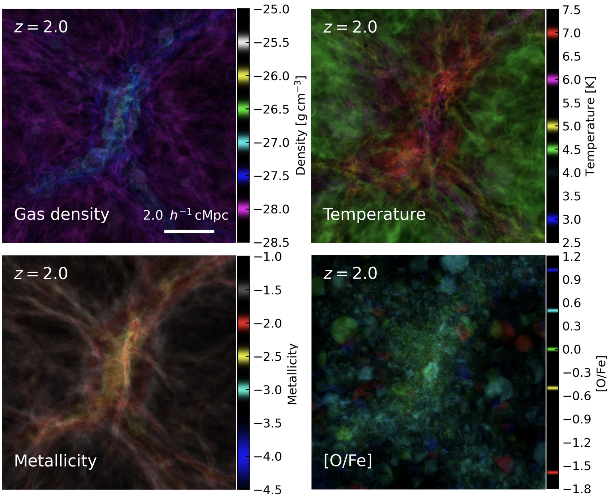
Figure 3 shows the volume rendering image of the simulated PC region () at in the M15-Gas run. These figures show the gas density, the gas temperature, the gas-phase chemical abundance [O/Fe], and the gas-phase metallicity, clockwise from the top left panel, respectively. Green, cyan, blue, and magenta colors in the gas isodensity surface indicate and , respectively. In the top right figure, the gases with gas temperatures of and are colored red, magenta, green, yellow, and blue, respectively. In the bottom left figure, the gases with gas-phase metallicity of and are colored red, yellow, cyan, and blue, respectively. In the bottom right figure, the gases with and are colored red, yellow, green, cyan, and blue, respectively.
The SPH particles are smoothed into cubic pixels using a quintic spline kernel (Morris 1996) before ray-tracing radiative transfer calculations are performed. The transfer functions for each figure are adapted by hand. The depth in each figure is also , and the transparency (alpha channel) is determined using the gas density.
3 RESULTS
3.1 Evolution of PC and Core
3.1.1 Evolution of Mass and Radius
Figure 4 shows the redshift evolution of the radius (in comoving Mpc) and mass () of the PC (dashed line), Core region (solid line) and Outside-core region (dotted line) in our zoom-in simulation (Thick red: M15-Gas, blue: M14.9-Gas, green: M14.7-Gas, purple: M14.4-Gas). The PC’s comoving radius from M15-Gas keeps getting shorter and shorter with redshift, but it always exceeds comoving Mpc until . All PCs have a radius of at least 10 cMpc at . On the other hand, the radius of the Core is monotonically increasing. The sharp increase of M15-Gas at and is due to the effect of the major mergers. At , the Core represents only of the entire volume of the PC. Thus, to examine the entire massive PC region, it is necessary to examine a wide area of more than , and it is not possible to reveal the entire picture by only examining the Core region. These results are consistent with those of Chiang et al. 2017.
The PC’s total mass was about in the M15-Gas run and it hardly changed over time. Other samples also show a similar trend. The definition of PC region, which utilizes the membership probability, presumes the tracking of the Lagrangian volume and affirms that the PC is successfully traced.
The mass in PC includes the mass in the Core region. The Core mass increased sharply from high- to low- due to the gas inflow into the Core and mergers, and it reached at for the M15-Gas run. The mass of M15-Gas at is slightly smaller than the mass of SPT2349–56 (Hill et al. 2020). Similarly to the radius evolution, the Core mass of M15-Gas shows a sharp increase at , 4.6, & 8.3, because of the major mergers with haloes of similar mass to the Core. The mass of the Outside-core for M15-Gas is higher than the Core even at , and the Core mass is less than half of the total PC mass. The Core reached at , and it represents of the total PC mass at . The Core mass of M14.9-Gas, M14.7-Gas, and M14.4-Gas reach half of the PC’s total mass at , , and , respectively. Also, the Core masses of the M14 sample are not always in the same order at each redshift, which shows the complex effect of gas inflow and mergers on Core growth.


3.1.2 Evolution of SFR
Figure 5 shows the redshift evolution of the total SFR (top panel) and metallicity (bottom) for the PC (dashed), Core region (solid), and Outside-core region (dotted) in our zoom-in simulations (Thick red: M15-Gas, blue: M14.9-Gas, green: M14.7-Gas, purple: M14.4-Gas). The SFR and metallicity in PC include the contribution of the Core region. In Lacaille et al. 2019, SFRs were derived for the two PCs in both the PC and Core regions. The Core value, representing the smaller value at each redshift, was obtained. The observed SFR values of Mitsuhashi et al. 2021; Kubo et al. 2019 are indicated for the PC with error bars. Additionally, the SFR from Lacaille et al. 2019 is shown for both PC and Core. Kubo et al. 2019’s study offers two estimates for the SFR: based on a pure star-forming model, and another at derived from the AGN/SFG composite model. In the study by Lacaille et al. 2019, SFRs were determined for the two PCs in both the PC and Core regions. The total SFR of Core corresponds to the smaller value at each redshift. The grey dotted curve shows the cosmic SFRD of Madau & Dickinson 2014 multiplied by the PC volume of M15-Gas. In the bottom panel, the triangle symbols correspond to the center of galaxy clusters (Balestra et al. 2007), and square symbols to IGM (Aguirre et al. 2008; Simcoe 2011; Simcoe et al. 2011).
The total SFR in the PC of M15-Gas continues to increase and reaches yr-1 at , and then decreases towards . The SFR in the Core region of M15-Gas increases sharply at , then after some ups and downs, it reaches a peak at with yr-1. At , the SFR of the cluster is , comparable to observations of nearby clusters(Kesebonye et al. 2023). The Outside-core region has a similar SFR to that of the PC up to , and the Core’s SFR reaches only of that of the PC. This fraction is higher than the result from Chiang et al. 2017 (). This discrepancy can be attributed to differences between the semi-analytic model and hydrodynamic simulations. In particular, our simulation does not account for AGN feedback, while their semi-analytic model incorporates an increased quiescent fraction for more massive galaxies by considering the influence of AGN feedback. This disparity in modeling approaches may lead to potential discrepancies in the SFR between the Core and PC regions. This suggests that it is necessary to study the entire PC and not just the Core to obtain a full SF history of PCs, which is consistent with the findings by Chiang et al. 2017. The PCs have 10 times higher SFR than expected from the cosmic mean (grey dotted line) inferred from Madau & Dickinson 2014.
The SFR of our PC is 0.92-2.4 (0.50-–1.21) times larger than that of Lacaille et al. 2019 at (), aligning with the observations. The SFR in our PC is also 0.44-0.92 times higher than the PC SFR determined by Kubo et al. 2019’s pure star-forming model, and it is 3.4-7.2 times higher than that estimated by their AGN/SFG composite model. We note that our simulations do not include AGN feedback, hence our results show a reasonable agreement with Kubo et al. 2019’s pure star–forming model. Our PC’s SFR is 2.6-5.5 times larger than that of Mitsuhashi et al. 2021’s result. This discrepancy might be attributed to the fact that our plotted data excludes contributions from galaxies other than SMGs. In the case of the Core, its SFR is 0.39-0.057 times lower than that of Lacaille et al. 2019 at and 0.71–0.20 times lower at . In section 3.1.4, we explore the reasons for the Core’s lower SFR in our simulations.

3.1.3 Evolution of Metallicity
The bottom panel of Fig. 5 and Figure 6 show that the PC’s metallicity continues to increase from high- to low-. The bottom figure represents the same figure as the middle panel, but with a focus on lower redshifts. Additionally, we have included the evolution of metallicity in the central region (). The square symbols show the observational result of IGM (Aguirre et al. 2008; Simcoe 2011; Simcoe et al. 2011), which might be closer to the mean metallicity of the universe at each redshift. Compared to the IGM metallicity, our simulated PCs have higher metallicities by more than .
The Core region’s metallicity of M15-Gas reaches higher than already at due to the star formation at . The Core’s metallicity of the M14 sample is also very high even at , because the Core at those redshifts is basically just one halo with a mass of enriched by the central galaxy to . This metallicity is consistent with observations (Curti et al. 2023) and simulations from IllustrisTNG (Nelson et al. 2019) and EAGLE (Schaye et al. 2015).
Core’s metallicity slowly decreases from to , which is due to the accretion of pristine gas (see also Appendix B). The result of high metallicity at early times in the Core region is consistent with observations (Baldi et al. 2007; Ettori et al. 2015; McDonald et al. 2016; Mantz et al. 2017). Some simulations (GADGET-3 and IllustrisTNG) found no time evolution of the central metallicity of PC (Biffi et al. 2017; Vogelsberger et al. 2018), while the Cluster-EAGLE simulation shows a decreasing metallicity similar to our simulations (Pearce et al. 2021).
The triangle symbols at represent the observed result of the cluster center (Balestra et al. 2007). In our simulation, the metallicity in the center of the Core is approximately 0.4 dex higher than in observation and simulations. We discuss the high metallicity in the center in Sec. 3.1.5. Observations show that the evolution of metallicity is not so rapid at (Baldi et al. 2012; Ettori et al. 2015; McDonald et al. 2016; Mantz et al. 2017).
Some simulations (GADGET-3 and IllustrisTNG) found no time evolution of the central metallicity of PC (Biffi et al. 2017; Vogelsberger et al. 2018), while the Cluster-EAGLE simulation shows a decreasing metallicity similar to our simulations (Pearce et al. 2021).
The observations (Yates et al. 2017) and other simulation results (Truong et al. 2019; Pearce et al. 2021) indicate that the metallicity in the center of the Core is lower for lower-mass clusters at . However, our results do not exhibit a clear trend, which could be attributed to the limited sample size.
Since the PC region is a Lagrangian volume, the PC mass is constant, as seen in Fig. 4. Therefore, the metallicity of the PC region can also be interpreted as the total mass of heavy elements if gas inflow/outflow is not significant in the Lagrangian volume. In addition, the stellar mass of the entire PC is almost constant at in our simulations. For these reasons, the heavy element mass has not increased much since , supporting early enrichment in the PC region (Ettori et al. 2015; McDonald et al. 2016; Biffi et al. 2018; Pearce et al. 2021). The metallicity of the PC at is mainly dominated by gas whose temperature is , which we show in Sec. 3.1.7.
3.1.4 Concentration of star formation
Figure 7 shows the total SFR in certain sky-area (top left: , top right: , bottom left: ). The bottom right panel shows the results of all three redshifts simultaneously. The ordinate indicates the total SFR within (on-sky area) within distance from the center using radial bins of size . The abscissa shows the sky area (in proper units). The thicker and darker lines indicate the M15-Gas run, and the thinner and lighter lines indicate M14.9-Gas, M14.7-Gas, and M14.4-Gas, respectively. The gray dashed lines and star symbols show the observed values (Hill et al. 2020). In the bottom right panel, purple, green, and red lines indicate and 2.0, respectively. The vertical lines in the each panel show the Core radius of M15-Gas at the indicated redshift.
The cumulative SFR is proportional to the area if galaxies are distributed uniformly. There is a plateau of SFR in the central region indicating the concentrated SFR in the center, more than expected from the extrapolation of an outer power-law distribution. There is no clear evolution in the cumulative SFR during . However, for all PCs, the increase in the cumulative SFR with increasing radius is slower at than at at larger radii ( pMpc2). This is an indication that the centralization of SFR is more advanced at . The cumulative SFR in the Outside-core region is consistent with the observed value at each redshift. Compared to the simulated cluster sample in Yajima et al. 2022, our sample seems to have a slightly higher SFR on large scales, although the central region has comparable SFR values.
Our simulations do not reproduce the Cores with very high SFRs at and 4.30 (Miller et al. 2018). This may be because the star formation is underestimated in our simulations due to insufficient resolution to resolve dense molecular gas where starbursts occur. Therefore, the region with a dense concentration of starburst galaxies in the Core center is not reproduced well, while the outer regions, dominated by main sequence galaxies, align with the observations.


|


|
3.1.5 Radial distribution
Galaxy clusters can be classified into two categories: those with a cool core, which contains cold gas in their central regions, and those without a cool core, known as non-cool core clusters. To clarify whether our cluster has a cool core or not, we examine the entropy of our simulated clusters at , where is Boltzmann’s constant, is the temperature of the gas, and is the number density of electrons. The lower left panel of Fig. 8 shows the radial profile of entropy normalized by and . Red, green, and blue lines are the results of the M14.9-Gas, M14.7-Gas, and M14.4-Gas at , respectively. The gray solid, dashed, and dotted lines are the median of the 31 clusters observed (Pratt et al. 2010), the EAGLE-like simulation results for massive clusters (their high-resolution run) (Altamura et al. 2023), and the entropy baseline profile from non-radiative simulations (Voit et al. 2005). All of our galaxy clusters have a cool-core with at which is below the observed data (Pratt et al. 2010) and the EAGLE-like simulation. Our slope is slightly shallower than Voit et al. 2005 model.
In our PC, cool cores exist even though a major merger has occurred at in M15-Gas. This merger is an event between a high-density, low-temperature massive halo and a cold, low-density central halo. Therefore, after the merger, there is a low-temperature, high-density Core, and the entropy of the Core is low. Note that this is just an example and further analysis is needed.
The top left panel of Figure 9 shows the radial profile of the mass-weighted temperature as a function of PC-centric radius normalized by . The purple (solid), blue (dashed), red (dotted), green (dash-dot), and black (dash-dot-dot) lines show the mean value from our PC sample at & , respectively. Star-shaped symbols are observed values by XMM–Newton at (Leccardi & Molendi 2008a). The mean temperatures ( mass average at ) of the most massive M15-Gas are and at and 1, respectively. For the least massive M14.4-Gas, at . Because of different masses, there is a large variation in the average temperature values, but the normalized temperature distribution does not show much difference.
At each redshift, the central temperature is lower than the peak temperature of each profile, reflecting the existence of cool-cores of the simulated clusters, which is observed for nearby galaxy clusters (Baldi et al. 2007; De Grandi & Molendi 2001; Leccardi et al. 2010). This trend did not change when plotting each cluster profile individually. However, while this trend qualitatively aligns, there remains a quantitative discrepancy as the simulated central temperature is approximately 1.5-2 dex as high as the observed temperature. Our simulation result of the mean temperature is dominated by the gas around , which is not measured in the observations. Therefore, shows a higher than observation. The M15-Gas cluster experiences a major merger at with another comparable cluster, but it still maintains a cool-core even after experiencing the major merger.
The upper right panel of Fig. 9 shows the radial profile of metallicity, specifically the Fe abundance normalized by solar Fe abundance . The purple, blue, red, green, and black lines show the average results of our simulated PCs at & 6, respectively. Star-shaped symbols are the observed values by XMM–Newton at (Leccardi & Molendi 2008b). The metallicity increases towards the PC center, and peaks at the center when the sample average is taken. This trend is consistent with the observed one in galaxy clusters with cool-cores (De Grandi & Molendi 2001; De Grandi et al. 2004; Baldi et al. 2007; Leccardi & Molendi 2008b; Johnson et al. 2011; Elkholy et al. 2015).
In clusters with cool-cores, the metallicity peak is at the center because heavy elements are trapped in a deep gravitational potential well, while in clusters with non-cool-cores, heavy elements are more widely distributed by the effects of a major merger and AGN feedback with off-center metallicity peak. The trend of the metallicity profile of clusters with the cool-core is consistent with other numerical results (Biffi et al. 2017). Some numerical simulations with AGN feedback show lower metallicity at the center and higher metallicity at the outside compared to the simulations with only SN feedback (Biffi et al. 2017; Choi et al. 2020). The reason for the steep slope in our simulation can be the lack of AGN feedback implementation.
The bottom two panels of Fig. 9 show the radial profile of O/Fe (left) and Si/Fe (right). The orange and green lines show the radial profile of O/Fe and Si/Fe in our simulation at . The differences in the line style show the different mass samples in our simulations. The solid, dashed, and dotted gray lines show the result from TNG100, TNG300 (Vogelsberger et al. 2018), and EAGLE (Pearce et al. 2021) simulations at , respectively. The darker gray lines show O/Fe, and weaker gray lines show Si/Fe in both TNG and EAGLE simulations. The black square and circle points show the observational results of O/Fe and Si/Fe from observation of AWM7 (Sato et al. 2008), Centaurus (Sakuma et al. 2011), and Coma (only Si/Fe) (Matsushita et al. 2013), respectively. We use following values of and to scale observed data and simulated data: (Sato et al. 2008) and (Pinto et al. 2015) for AWM7; (Markevitch et al. 1998; Furusho et al. 2001) and (Pratt et al. 2010; Pointecouteau et al. 2005; Walker et al. 2013) for Centaurus cluster; (Evrard et al. 1996; Markevitch et al. 1998) and (Planck Collaboration et al. 2013; Matsushita et al. 2013) for Coma cluster.
Our chemical abundance profile is almost constant, which is in good agreement with observations and EAGLE simulation. The TNG simulation showed a slightly increasing trend with radius. Our [Si/Fe] profile shows consistency with observed values, but [O/Fe] is 0.3 dex smaller than observed values. The difference in this trend is influenced by the specific methods and parameters used to treat feedback processes, such as AGN feedback and kinetic SN feedback. These feedback mechanisms can impact the rate of gas outflow from galaxies, and the SFR of galaxies. Ultimately, they can modify the abundance ratio of alpha/Fe in the intracluster medium.


3.1.6 Different phases of gas
The top panel in Figure 10 is the phase diagram of M15-Gas run weighted by gas mass at , showing how much gas mass is in which phase. Since the M15-Gas run is a zoom-in simulation, it shows mainly the gas in the PC region. We define four gas phases of ‘Hot’, warm-hot intergalactic medium (WHIM), ‘Diffuse’, and ‘Condensed’. The Hot phase is the gas with temperatures K, which includes the gas that has been heated by the SN feedback and those that reached a high virial temperature in the Core region. We define the WHIM phase as the gas with K (Shull et al. 2012, c.f.), and the Diffuse phase by K and gas densities g cm-3. The Condensed phase is defined by K and g cm-3.
The bottom panel is a visual image of the M15-Gas run at , with red, magenta, green, and blue colors indicating the Hot, WHIM, Diffuse, and Condensed phases, respectively. The Hot phase exists in the Core, and WHIM is distributed along the filaments. The Diffuse phase is spread over the low-density region, and the Condensed phase is too small to be seen in this figure.
Nelson et al. 2018 examined the oxygen ion emission using IllustrisTNG simulations and found that the lowest observed O vi column density of cm-2 (Danforth & Shull 2008; Danforth et al. 2016) corresponds to Mpc (physical) based on the simulated density profile (their Fig. 9). This corresponds to comoving 30 Mpc at , covering the entire PC region of our simulation. Given that we are also interested in probing denser gas in the Condensed phase, here we choose to analyze all the gas in the entire PC region of comoving Mpc as shown in Figure 10.
3.1.7 Chemical abundance evolution in PC and Core
Figure 11 shows the redshift evolution of chemical abundance ([Fe/H] and [O/Fe]) in the PC for four gas phases of ‘Hot’ (red), warm-hot intergalactic medium (WHIM; purple), ‘Diffuse’ (green), and ‘Condensed’ (blue). The median of the entire sample is shown as a dashed line, and the variance is shown by a shade, using M15-Gas, M14.9-Gas, M14.7-Gas, and M14.4-Gas run at , and M14.9-Gas, M14.7-Gas and M14.4-Gas for .
In the top panel of Figure 11, the metallicity (as represented by [Fe/H]) increases with decreasing redshift, consistently with increasing star formation from high- to low-. The gray line is the same as the average metallicity of the PC region in the lower panel of Fig. 5. At , the metallicity of the hot phase coincides with the total metallicity; at , of the heavy elements and of the total gas mass are present in the Hot phase. The Hot phase is heated by both the virial shock in massive systems and SN feedback, and its metallicity is roughly constant at even at high redshift. The Hot and WHIM phases in the PC are already highly enriched even at due to SN feedback. The red dashed line for the Hot phase is discontinuous at , which is due to the lack of this phase at this high-. The Condensed phase catches up with the WHIM at and with the Hot phase at . The Diffuse component has the lowest [Fe/H] among all phases as it corresponds to unenriched IGM. However, at , its [Fe/H] experiences a significant increase. This rise can be attributed to the Condensed phase gas being heated and contaminated by metals due to feedback processes. As the gas passes through the Diffuse phase, it eventually reaches the WHIM phase.
The bottom panel of Figure 11 shows that [O/Fe] decreases from at high– to at . This is because SN II is associated with massive star explosions and therefore occurs earlier than SN Ia, which leads to more abundant oxygen than iron at the PC and Core in the early universe. In other words, [O/Fe] decreases with time.

Figure 12 shows [O/Fe] vs. [Fe/H] for different gas phases in the Core and Outside-core. The color of each line is the same as in Fig. 11. The metallicities of Condensed and WHIM phases are higher in the Core region than in the Outside-core at the same [O/Fe]. This is because the star formation is more active in the Core than in the Outside-core, which is consistent with Fig. 5, with the exception of the Hot phase, which is enriched by the early SN feedback events at high-. The timing at which the slope changes in Fig. 12 is when the ratio of SN Ia to SN II changes. As SN Ia begins to enrich the Core region’s Condensed phase at , [O/Fe] sharply drops towards .


3.1.8 Chemical pattern
Figure 13 shows the evolution of the chemical pattern of Cores in our simulations. The shade indicates the sample variance (). The chemical abundance of the observed Perseus clusters (Hitomi Collaboration et al. 2017) and 44 systems (cluster, group, ellipticals) (Mernier et al. 2018) is consistent with the solar abundance. Each point is shifted slightly in the x-axis direction to avoid overlap. The oxygen and -element such as Ne and Mg are ejected from SN II, Ni and Fe are from SN Ia, and Si, S, and Ca are from both. When stars are young, more -elements are produced than Fe, but as the stars become older, more Fe are produced by SN Ia, and /Fe decreases as we can see in the evolution from to for O, Ne, Mg, Si, S, and Ca.
Similarly, the abundance evolution of any -element reaches solar abundance at and does not evolve much from to . The [X/Fe] ratios for alpha elements originating from SN II are lower compared to observations, while the [Ni/Fe] ratio for Ni originating from SN Ia is higher. This suggests that the contribution of SN Ia to Fe may be overestimated in our calculation, as Fe is predominantly sourced from SN Ia with a smaller contribution from SN II. The DTD offset of SN Ia is , and if the offset is set to or so, the produced Fe abundance may decrease and meet the observation. However, SN Ia and galaxy clusters observations and the theory of binary population synthesis should determine this offset (Maoz et al. 2014). Also, since Fe is more easily incorporated into dust than -elements, combining realistic dust handling in our simulations may lead to a better agreement on -element abundance.
As for the elements of SN Ia origin, especially Ni, it is difficult to see any difference or evolution because Fe also has the same origin. However, it is still not very consistent with solar abundance as observed. Introducing a yield table for SN Ia or dust model may be necessary.
Other observations show that [O/Fe], [Ne/Fe], and [Mg/Fe] in the Centaurus cluster are below the solar abundance (0.4 dex) as in our results, but [Si/Fe], [S/Fe], and [Ca/Fe] are almost at the solar abundance (Fukushima et al. 2022). They also show [Ni/Fe] , which is consistent with our results. They also show [Ni/Fe] , which is consistent with our results. They used an SN nucleosynthesis model and showed that the low [/Fe] could be reproduced, but high [Ni/Fe] could not be reproduced from the linear combination of SN II and SN Ia, but our calculation does. Therefore, we argue that it is necessary to consider the contribution of gas dynamics in galaxy clusters to the chemical abundance ratios and realistic star formation histories.
Most Observational data are obtained near the center of galaxy clusters, whereas our simulation results are based on data from the entire Core. Observations suggest that the chemical abundance is relatively constant from the center to the outskirts of galaxy clusters or groups (Tokoi et al. 2008; Komiyama et al. 2009; Sasaki et al. 2014; Mernier et al. 2017). Therefore, the difference in the region used for taking the data is unlikely to be the main reason for the discrepancies.
3.2 Galaxies in PC
We now shift our attention from the gas to the galaxies in our simulated PCs.
3.2.1 MZR
Figure 14 shows the stellar mass—metallicity relation (MZR) at . Our simulation results (M14.9-Gas, M14.7-Gas, M14.4-Gas) are plotted as a scatter plot, and the observational data are plotted as a scatter plot with errors (Sanders et al. 2021, with a median of ) and the shaded region (Strom et al. 2022, with a mean of ). These two observations differ in the estimation method of metallicities from emission lines. The gas metallicity and stellar masses are determined from the SPH and stellar particles within twice the half-stellar mass radius of each galaxy.
Our results show a steeper or comparable slope compared to the observations of Strom et al. 2022 and Sanders et al. 2021, respectively. Different colors of data points show different regions of PCs, but those data points all overlap with each other, suggesting that the environmental differences in MZR are not seen in our simulated PC regions. Our results are consistent with several observations showing no environmental effects on the MZR (Kacprzak et al. 2015; Namiki et al. 2019; Calabrò et al. 2022).

3.2.2 Chemical abundance evolution in galaxies
Figure 15 shows (N/O) versus (O/H) of galaxies at . Red, blue, and black points indicate galaxies in different regions of the Core, Outside-core, and Outside-PC, respectively. Each chemical abundance is determined from the SPH particles that are within twice the half-stellar mass radius of each galaxy. The cyan square symbols with errors are from Steidel et al. 2016, and the magenta star-shaped symbols are from Kojima et al. 2017 observations. The vertical and horizontal black dotted lines indicate the solar values. As we saw in Section 3.2.1, massive galaxies have higher metallicity, so the horizontal axis correlates with the stellar mass of galaxies. Low-metallicity galaxies tend to have more O than N, i.e., lower N/O. As we see in Fig 19 in Appendix A, N is the AGB star origin, and O is the SN II origin; therefore, young galaxies or galaxies with increasing SFR are expected to have low (N/O), while older galaxies or galaxies with decreasing SFR are expected to have high (N/O). In our simulation, galaxies with higher N/O are older when stellar mass is fixed. Details are discussed in Sec. 4.4.
There is not much difference in the values of (N/O) according to the environment that the galaxies live in. The observed value of (N/O) in the field (Steidel et al. 2016; Kojima et al. 2017) is almost the same as that of our simulations.

4 Discussions
4.1 The origin of the peak in total star formation
We saw in Figure 5 that the SFR peaks at different redshifts for the Core region () and the PC region (). To understand what causes this difference, we investigate the contribution to global star formation by galaxies with different stellar masses.
The top panel of Figure 16 shows the time evolution of the number of galaxies in each stellar mass range in M15-Gas. The solid and dashed lines indicate the galaxies in the PC and Core, respectively. Note that the PC line includes the contribution from the Core. In our PC, the number of galaxies with continues to increase from high- to , but then slightly decreases at . At high redshifts (, the slope of the stellar mass function for low-mass galaxies is steeper than at (Genel et al. 2014; Furlong et al. 2015; Pillepich et al. 2018b). In particular, the FIRE simulation demonstrates that the stellar mass function at is higher than that at for galaxies with stellar masses less than (Feldmann et al. 2023). These findings align with a decrease in the number density of lower stellar masses. In the Core, the number of galaxies in any mass range does not decrease. The discussion of the effect of tidal disruption is a topic for future research.
The bottom panel in Fig. 16 shows the redshift evolution of the ratio of the sum of the SFR of galaxies in each stellar mass range to the total SFR of Core and PC, respectively. The different colors indicate different stellar mass ranges of the galaxy at each redshift as indicated in the legend, divided by . We find that the lower mass galaxies dominate the total SFR at earlier times, because they form first in the CDM universe. Our simulation shows that low-mass galaxies with account for of the total SFR in the PC at . When the total SFR of the PC is highest (), galaxies with account for over half of the PC’s SFR (). In contrast, at , where the total SFR of the Core is highest, the SFR of galaxies with accounts for of the total SFR. The peak of the SFR for PC and Core is caused by the quenching of star formation in low-mass galaxies, and the SFR peak for the Core region is delayed compared to the PC, because the Core is relatively more affected by the massive galaxies’ star formation. In our simulation, we observe a delay in the quenching of lower stellar mass galaxies in the PC compared to the Core, indicating the occurrence of environmental quenching. This quenching in low-mass galaxies may be caused by SN feedback, tidal effect (Moore et al. 1996), ram pressure stripping (Gunn & Gott 1972), and/or strangulation (Larson et al. 1980).


4.2 Comparison with other simulations
Pearce et al. 2021 find that the metallicity in galaxy clusters decreases with redshift at using the Cluster-EAGLE simulations (Bahé et al. 2017; Barnes et al. 2017). They also used a large cosmological box (), and found massive galaxy clusters with . The lower limit of the mass range is similar to ours, and the upper limit is more massive than ours owing to their larger box size. They found that the metallicity decreases with redshift, which agrees well with our result of the Core region Fig. 5. The metal abundance of the Core region in our simulations also decreases from high- to low- due to primordial gas inflow.
As seen in the bottom panel of Fig. 9, the slope of the Si/Fe and O/Fe radius profiles in our simulations agree with observations and Cluster-EAGLE simulations. Our galaxy clusters show low slope values for [O/Fe], ranging from 0.06 to 0.12, while the TNG simulations exhibit slopes of approximately 0.27 to 0.4. The EAGLE simulations, on the other hand, display a slope of 0.1. Mernier’s study reports a slope of around -0.002. In the case of [Si/Fe], our samples exhibit slopes ranging from 0.09 to 0.13, while the TNG simulations display slopes between 0.23 and 0.35. The EAGLE simulations show a slope of 0.10, while Mernier’s observation reports a slope of -0.16. The different slope from TNG100 might be due to the absence of AGN feedback or differences in the SN feedback model. It is possible that SN Ia occurs more effectively in the Outside-core region of our simulation than in TNG100. The normalization of fitting function for Si/Fe of our simulation, TNG100, Cluster-EAGLE, and Mernier’s observation are 1.25, 2.0, 2.13, and 0.64. Our simulations reproduce the observed Si/Fe better than TNG100 and Cluster-EAGLE simulations. For O/Fe, there is an excess of Fe relative to O, although our results are consistent with observations within the errors. It is possible that more SN Ia is occurring relative to SN II, and further analysis is needed.
As we saw in the Fig. 8, all of our galaxy clusters have a cool-core with at which is below the observed data (Pratt et al. 2010) and the EAGLE-like simulation (Altamura et al. 2023). Our slope is slightly shallower than Voit et al. 2005 model. According to Altamura et al. 2023, the presence or absence of AGN feedback changes the entropy profile only slightly. Altamura et al. 2023 uses SPHENIX SPH (Borrow et al. 2022) as their SPH scheme, and we use the density–independent formulation of SPH (DISPH) (Saitoh & Makino 2013), which may cause the discrepancy. The Santa Barbara Cluster Comparison Project (Frenk et al. 1999) showed that the SPH code does not generate an entropy core, and there is a systematic discrepancy with the mesh code. However, in the idealized simulation of Saitoh 2016, DISPH can generate an entropy core similar to quasi-Lagrangian schemes such as moving-mesh and mesh-free methods. Therefore, it is possible that the cool-cores in our simulations are due to SN feedback or the formation process of galaxy clusters rather than numerical methods. To address this issue, it is necessary to simulate the same cluster using the same physics model but with a different numerical scheme. Additionally, the effects of thermal and kinetic SN feedback on star formation and the physical properties of the intracluster medium should be considered carefully, and we need to perform additional simulations with different feedback models. These simulations will be part of our future work.
4.3 MZR as a test of the model
Figure 17 shows the MZR of galaxies at in M14.4-Gas (solid line) and M14.4-SNIa1e8 (dashed line) for the elements O, Fe, and N in blue, red, and green, respectively. We fit our MZR using the following equation from Curti et al. 2020:
| (1) |
Equation (1) approaches for , and for , the power-law slope becomes . If is large, the bend is sharper. Table 2 shows the coefficients and their errors when a non-linear fit is performed using the least squares method. The observation by Strom et al. 2022 is shown by the dotted line and the shade; the slope and dispersion for O and Fe are almost identical, indicating that the origin of Fe in high- galaxies is SN II and that alpha enhancement is seen. Due to the low gas fractions in our samples, the metallicity is higher compared to the observations.
The difference between the O–MZR and Fe–MZR slopes at lower stellar mass depends on the SFH, galaxy ages, and the timescale on which SN Ia occurs. When the galaxy has an increasing SFH or is young, SN II becomes more effective, and the O- and Fe–MZR slopes are almost identical. Increasing the timescale of SN Ia reduces Fe contamination from older stars and makes the Fe–MZR slope shallower; therefore, we expect M14.4-SNIa1e8 run to have a shallower slope than M14.4-Gas. Our results exhibit higher values than the observations in Strom et al. 2022. Furthermore, the observed slopes are shallower in comparison. This discrepancy can be attributed to the inefficiency of SN feedback, particularly for massive galaxies in our simulations. As a result, our simulation tends to overproduce stellar mass, leading to a lower gas fraction in galaxies. This imbalance contributes to higher metallicity levels than observed galaxies. In addition, the Fe–MZR has a steeper slope than the O–MZR, which might be because the galaxies in our sample are older and have decreasing SFHs at . The M14.4-SNIa1e8 result also shows a steep slope of Fe–MZR, which is against our original expectations. The increase in SN II-derived Fe relative to SN Ia-derived Fe brings the slope of the Fe–MZR closer to that of the O–MZR. Thus, the uncertainty of DTD offset should be considered in any future discussion of chemical evolution using MZR of Fe or other elements.
From the O- and Fe–MZRs of M14.4-Gas and M14.4-SNIa1e8 at , we estimate and , respectively. This corresponds to and times the , respectively. This is lower than the Strom et al. 2022 result ( for ) but higher than the solar abundance. This may be because enhancement occurs at higher redshifts for high-density galaxies and gradually approaches the solar abundance at .
In Table 2, we see that the dispersion for N/H and Fe/H are larger than O/H, which could be due to the contribution by AGB and SN Ia to N and Fe, respectively, consistent with Strom et al. 2022.

| Element | |||||
|---|---|---|---|---|---|
| M14.4-Gas | |||||
| M14.4-SNIa1e8 | |||||
4.4 Dispersion in the N/O–metallicity diagram
The gas phase chemical abundances of galaxies are important to understand galaxy evolution and gas dynamics. Galaxy metallicity correlates with gas inflow, outflow, and metal enrichment from stars, while chemical abundance correlates with the ratio of SN II, SN Ia, and AGB, i.e., SFH. For example, in a simple one-zone closed box model, N/O has a low abundance in the low-metallicity galaxy and a high abundance in the high-metallicity galaxy. This is because oxygen is the primary element and nitrogen is the almost secondary element. However, observationally, it is known that the relation between (N/O) and metallicity have a large scatter at low metallicities. The MaNGA (Mapping Nearby Galaxies at APO) survey, which studies the gas inside nearby galaxies using large integral field spectroscopy, shows similar results (Belfiore et al. 2015). These results indicate that the dispersion of N/O in low-metallicity galaxies may be a tracer of gas inflow. Luo et al. 2021 suggested that the inflow of metal-poor gas into the disk with high metallicity and high N/O can create large dispersions. Berg et al. 2020 suggested that differences in SFH change the evolution of N/O and that the low metallicity regions have lower abundances for galaxies with higher past star formation efficiency.
To investigate the origin of the large N/O dispersion in low-metallicity galaxies at (see Fig.15), we divide the galaxies in the range of and into the following three subsamples and examine their respective SFH: high (), medium (), and low (). Figure 18 shows SFHs for the high (red), medium (black), and low (blue) N/O galaxies. The solid line shows the median value for each subsample, and the dashed line shows the mean value. The colored data points at show the observational results of log(N/O) for each SFR bin from Hayden-Pawson et al. 2022. Galaxies with high N/O at have low SFRs, consistent with observations. The galaxies with low N/O have continuously increasing SFH, while those with high N/O have a peak in SFR at . This contradicts the results of Berg et al. 2020 that galaxies with higher past SFR have lower N/O. Luo et al. 2021 argued that the inflowing gas reduces O/H while keeping N/O roughly the same. Then the SFR would be higher in galaxies with high N/O if inflow induces further star formation. However, our simulations show the opposite, suggesting that SFH is a more dominant cause for large N/O dispersion than gas inflow.

Some observations found that galaxies have a different distribution from local galaxies (Shapley et al. 2005; Erb et al. 2006; Steidel et al. 2014; Kojima et al. 2017, e.g.,) in the BPT diagram (Baldwin et al. 1981), i.e., the so-called BPT offset. Kojima et al. 2017 provided two possible reasons that can explain the BPT offset between high- and low- populations. First, if galaxies have higher , they would have higher and lower , i.e., occupying the upper left side of the BPT diagram. Second, galaxies with high N/O would have higher and occupy the right-hand-side of the BPT diagram. Those in the middle can result from the combined effect of both N/O and .
In our simulations, the galaxies with low N/O in Fig. 18 have high SFRs at and thus high . In our simulations, the galaxies with low N/O in Fig. 18 have high SFRs and high density at and thus galaxies could have high . The SED calculation of stars or radiative transfer calculation of ionizing photons from massive stars is our future project. The simulated galaxies with high N/O had active star formation in the past, but their star formation declines from toward (Fig. 18).
4.5 Effects of AGN and dust
The galaxies in our simulation do not show signs of strong quenching of star formation, in contradiction to some observations of post-starburst galaxies (Gobat et al. 2012; Glazebrook et al. 2017; Schreiber et al. 2018; D’Eugenio et al. 2020; Valentino et al. 2020; Forrest et al. 2020a; Forrest et al. 2020b; Saracco et al. 2020; Kalita et al. 2021). This may be because our simulation does not include AGN feedback, which will be our future work. The introduction of AGN feedback is expected to alter the MZR of massive galaxies, and this may resolve the discrepancy with observations in Figs. 14 and 17.
Heavy elements are incorporated into dust, but we have not included any dust models this time. Incorporating a dust model into our simulations could change the amount of metal. In addition, each element has a different rate of incorporation into dust. For example, Calura et al. 2008 showed that Fe is incorporated into dust more than O and other elements. This effect increases the enhancement of our high- galaxies and may make the absolute value of Fe–MZR consistent with observations. We plan to investigate the effect of dust on the metallicity and the spatial distribution of dust using Gadget4-Osaka (Romano et al. 2022b; Romano et al. 2022a) in the future.
5 Conclusions
We examined the star formation and chemical enrichment in PCs using cosmological zoom-in hydrodynamic simulations by GADGET3-Osaka (Shimizu et al. 2019; Nagamine et al. 2021), including box size to reproduce a massive PC. We examined the chemical abundance and SFRs in PC and Core regions (see Sec 2.3 for their definitions). Our main results are summarized as follows:
- •
We defined the Lagrangian volume of galaxy clusters as the PC region and the massive central halo as the Core. The radius of all PC reaches at , covering a significant fraction of cosmological volume. In particular, M15-Gas have a radius up to until . The total mass (including both dark matter and gas) of the Core of M15-Gas is at , which corresponds to of the PC, and becomes at . For M14.9-Gas, M14.7-Gas, and M14.4-Gas, our results show that the most massive galaxy cluster at is not always the most massive Core at high- (Fig. 4).
- •
The total SFR in the simulated PC reaches at , with the Core region accounting for about half of the star formation in the PC at (top panel of Fig. 5). We find that the galaxies with at contributes about 50% of the total SFR of PC, while massive galaxies () dominate the total SFR of the Core at . The peak of total SFR for the PC and the Core is at different redshifts for galaxies with different masses (bottom panel of Fig. 16); lower mass galaxy sample peaks earlier.
- •
The cumulative SFR of Outside-core is consistent with the observed values at each redshift and is more centrally concentrated at than at (Fig. 7). However, there is no central concentration of very high SFR in the Core, as seen in the observations. This is because our simulation cannot reproduce starburst galaxies with extremely high SFR. This could be attributed to either insufficient resolution in our simulations or an inadequate understanding of the mechanisms governing star formation processes.
- •
- •
We divided the gas in the Lagrangian volume of PC into Hot, WHIM, Diffuse, and Condensed phases, and studied the chemical abundance evolution in each phase. The Hot and WHIM phases have high Fe/H even at . The Diffuse phase (i.e., the IGM) has lower Fe/H until than other phases, after which it catches up quickly and even supersedes that of Hot and WHIM at (Fig. 11).
- •
- •
The radial profile at reproduces the observations well in terms of temperature, metallicity, and Si/Fe, except for the inner profile of temperature. Our simulated clusters have cool-cores in the entropy profile. The flat slope of O/Fe agrees with the observations. Still, it is quantitatively slightly below (consistent within the errors), so future tests with different SN Ia/SN II ratios and yields are needed (Fig. 9).
- •
We compare the chemical abundance in individual galaxies with observations and find that the MZR shows a steeper or similar slope compared to observations. This is because the SN feedback is not effectively suppressing star formation in our simulations, leading to excessive star formation and a low gas fraction. Furthermore, our simulations do not show any environmental effects on MZR (Fig. 14). The N/O of the galaxies is consistent with observations and does not show any environmental variations (Fig. 15). An examination of the origin of the N/O dispersion revealed that galaxies with high N/O had active star formation in the past, while galaxies with low N/O had ongoing active star formation (Fig. 18).
- •
We changed the DTD offset of SN Ia to assess the sensitivity of the chemical enrichment result to this parameter. The slope of Fe–MZR did not change, but the metallicities decreased with a longer DTD offset in our M14.4-SNIa1e8. The [O/Fe] values of yr and yr for the DTD offset are 0.14 and 0.2, suggesting that the longer DTD offset is more consistent with the observation, although it does not reach the observed value of 0.35. Still, the Fe–MZR also depends on the SFH and age of the galaxy; therefore, we plan to study this dependency using simulations with different SN feedback models in the future. (Fig. 17).
Future missions will be able to observe protoclusters and obtain the corresponding data presented in this paper. For example, X-Ray Imaging and Spectroscopy Mission (XRISM) will be able to observe clusters at intermediate redshifts with sufficiently long observation times ( ksec). In galaxy clusters up to , XRISM can measure the Fe abundance with a significance of . It might be possible to observe the Si abundance up to and O abundance up to in some galaxy clusters (Kitayama et al. 2014; XRISM Science Team 2020). The X-ray Integral Field Unit (Barret et al. 2018, X-IFU;) onboard Athena (Nandra et al. 2013) will be able to observe spatially resolved chemical abundances in galaxy clusters and measure radial profiles, thereby providing constraints on the feedback effects (Simionescu et al. 2019).
Spectroscopic observations by the Subaru Prime Focus Spectrograph (PFS) will begin in (Greene et al. 2022), and many PCs will be identified spectroscopically. Metal absorption lines of various elements will also be observed, from which we can further understand the environmental effect of SFH at high redshift and the chemical evolution of the universe. By comparing the results of cosmological hydrodynamic simulations and observations, we can constrain the details of SN feedback model and chemical yield model. Our work will help reveal the chemical enrichment in the Universe, particularly using PCs as unique probes of accelerated structure formation and evolution.
Acknowledgements
We are grateful to Volker Springel for providing the original version of GADGET-3, on which the GADGET3-Osaka code is based. We also thank Takayuki Saitoh and Yutaka Hirai for the useful discussion on the CELib output. Numerical computations were carried out on the Cray XC50 at the Center for Computational Astrophysics, National Astronomical Observatory of Japan, and the OCTOPUS and SQUID at the Cybermedia Center, Osaka University, and the OakForest-PACS as part of the HPCI system Research Project (hp190050, hp200041, hp220044). This work is supported in part by the MEXT/JSPS KAKENHI grant numbers 19H05810, 20H00180, 22K21349 (K.N.). This work was supported by JST SPRING, grant number JPMJSP2138 (K.F.). K.N. acknowledges the travel support from the Kavli IPMU, World Premier Research Center Initiative (WPI), where part of this work was conducted.
DATA AVAILABILITY
Data related to this publication and its figures are available on request from the corresponding author.
References
- Aguirre et al. (2008) Aguirre A., Dow-Hygelund C., Schaye J., Theuns T., 2008, ApJ, 689, 851
- Alberts & Noble (2022) Alberts S., Noble A., 2022, Universe, 8, 554
- Altamura et al. (2023) Altamura E., Kay S. T., Bower R. G., Schaller M., Bahé Y. M., Schaye J., Borrow J., Towler I., 2023, MNRAS, 520, 3164
- Bahé et al. (2017) Bahé Y. M., et al., 2017, MNRAS, 470, 4186
- Baldi et al. (2007) Baldi A., Ettori S., Mazzotta P., Tozzi P., Borgani S., 2007, ApJ, 666, 835
- Baldi et al. (2012) Baldi A., Ettori S., Molendi S., Balestra I., Gastaldello F., Tozzi P., 2012, A&A, 537, A142
- Baldwin et al. (1981) Baldwin J. A., Phillips M. M., Terlevich R., 1981, PASP, 93, 5
- Balestra et al. (2007) Balestra I., Tozzi P., Ettori S., Rosati P., Borgani S., Mainieri V., Norman C., Viola M., 2007, A&A, 462, 429
- Bamford et al. (2009) Bamford S. P., et al., 2009, MNRAS, 393, 1324
- Barnes et al. (2017) Barnes D. J., et al., 2017, MNRAS, 471, 1088
- Barret et al. (2018) Barret D., et al., 2018, in den Herder J.-W. A., Nikzad S., Nakazawa K., eds, Society of Photo-Optical Instrumentation Engineers (SPIE) Conference Series Vol. 10699, Space Telescopes and Instrumentation 2018: Ultraviolet to Gamma Ray. p. 106991G (arXiv:1807.06092), doi:10.1117/12.2312409
- Belfiore et al. (2015) Belfiore F., et al., 2015, MNRAS, 449, 867
- Berg et al. (2020) Berg D. A., Pogge R. W., Skillman E. D., Croxall K. V., Moustakas J., Rogers N. S. J., Sun J., 2020, ApJ, 893, 96
- Biffi et al. (2017) Biffi V., et al., 2017, MNRAS, 468, 531
- Biffi et al. (2018) Biffi V., Mernier F., Medvedev P., 2018, Space Sci. Rev., 214, 123
- Borrow et al. (2022) Borrow J., Schaller M., Bower R. G., Schaye J., 2022, MNRAS, 511, 2367
- Boylan-Kolchin et al. (2009) Boylan-Kolchin M., Springel V., White S. D. M., Jenkins A., Lemson G., 2009, MNRAS, 398, 1150
- Calabrò et al. (2022) Calabrò A., et al., 2022, A&A, 664, A75
- Calura et al. (2008) Calura F., Pipino A., Matteucci F., 2008, A&A, 479, 669
- Campbell & Lattanzio (2008) Campbell S. W., Lattanzio J. C., 2008, A&A, 490, 769
- Casey (2016) Casey C. M., 2016, ApJ, 824, 36
- Chabrier (2003) Chabrier G., 2003, PASP, 115, 763
- Chiang et al. (2013) Chiang Y.-K., Overzier R., Gebhardt K., 2013, ApJ, 779, 127
- Chiang et al. (2017) Chiang Y.-K., Overzier R. A., Gebhardt K., Henriques B., 2017, ApJ, 844, L23
- Choi et al. (2020) Choi E., Brennan R., Somerville R. S., Ostriker J. P., Hirschmann M., Naab T., 2020, ApJ, 904, 8
- Contini et al. (2016) Contini E., De Lucia G., Hatch N., Borgani S., Kang X., 2016, MNRAS, 456, 1924
- Curti et al. (2020) Curti M., Mannucci F., Cresci G., Maiolino R., 2020, MNRAS, 491, 944
- Curti et al. (2023) Curti M., et al., 2023, MNRAS, 518, 425
- D’Eugenio et al. (2020) D’Eugenio C., et al., 2020, ApJ, 892, L2
- D’Eugenio et al. (2021) D’Eugenio C., et al., 2021, A&A, 653, A32
- Danforth & Shull (2008) Danforth C. W., Shull J. M., 2008, ApJ, 679, 194
- Danforth et al. (2016) Danforth C. W., et al., 2016, ApJ, 817, 111
- Davis et al. (1985) Davis M., Efstathiou G., Frenk C. S., White S. D. M., 1985, ApJ, 292, 371
- De Grandi & Molendi (2001) De Grandi S., Molendi S., 2001, ApJ, 551, 153
- De Grandi et al. (2004) De Grandi S., Ettori S., Longhetti M., Molendi S., 2004, A&A, 419, 7
- Doherty et al. (2014) Doherty C. L., Gil-Pons P., Lau H. H. B., Lattanzio J. C., Siess L., 2014, MNRAS, 437, 195
- Dressler (1980) Dressler A., 1980, ApJ, 236, 351
- Efstathiou et al. (1990) Efstathiou G., Sutherland W. J., Maddox S. J., 1990, Nature, 348, 705
- Elkholy et al. (2015) Elkholy T. Y., Bautz M. W., Canizares C. R., 2015, ApJ, 805, 3
- Erb et al. (2006) Erb D. K., Shapley A. E., Pettini M., Steidel C. C., Reddy N. A., Adelberger K. L., 2006, ApJ, 644, 813
- Ettori et al. (2015) Ettori S., Baldi A., Balestra I., Gastaldello F., Molendi S., Tozzi P., 2015, A&A, 578, A46
- Euclid Collaboration et al. (2023) Euclid Collaboration et al., 2023, A&A, 671, A100
- Evrard et al. (1996) Evrard A. E., Metzler C. A., Navarro J. F., 1996, ApJ, 469, 494
- Feldmann et al. (2023) Feldmann R., et al., 2023, MNRAS, 522, 3831
- Forrest et al. (2020a) Forrest B., et al., 2020a, ApJ, 890, L1
- Forrest et al. (2020b) Forrest B., et al., 2020b, ApJ, 903, 47
- Frenk et al. (1999) Frenk C. S., et al., 1999, ApJ, 525, 554
- Fukushima et al. (2022) Fukushima K., Kobayashi S. B., Matsushita K., 2022, MNRAS, 514, 4222
- Furlong et al. (2015) Furlong M., et al., 2015, MNRAS, 450, 4486
- Furusho et al. (2001) Furusho T., et al., 2001, PASJ, 53, 421
- Gao et al. (2022) Gao F., Wang L., Ramos Padilla A. F., Clements D., Farrah D., Huang T., 2022, A&A, 668, A54
- Genel et al. (2014) Genel S., et al., 2014, MNRAS, 445, 175
- Gil-Pons et al. (2013) Gil-Pons P., Doherty C. L., Lau H., Campbell S. W., Suda T., Guilani S., Gutiérrez J., Lattanzio J. C., 2013, A&A, 557, A106
- Glazebrook et al. (2017) Glazebrook K., et al., 2017, Nature, 544, 71
- Gobat et al. (2012) Gobat R., et al., 2012, ApJ, 759, L44
- Greene et al. (2022) Greene J., Bezanson R., Ouchi M., Silverman J., the PFS Galaxy Evolution Working Group 2022, arXiv e-prints, p. arXiv:2206.14908
- Guetta & Della Valle (2007) Guetta D., Della Valle M., 2007, ApJ, 657, L73
- Gunn & Gott (1972) Gunn J. E., Gott J. Richard I., 1972, ApJ, 176, 1
- Gunn & Tinsley (1975) Gunn J. E., Tinsley B. M., 1975, Nature, 257, 454
- Haardt & Madau (2012) Haardt F., Madau P., 2012, ApJ, 746, 125
- Hahn & Abel (2011) Hahn O., Abel T., 2011, MNRAS, 415, 2101
- Hayden-Pawson et al. (2022) Hayden-Pawson C., et al., 2022, MNRAS, 512, 2867
- Higuchi et al. (2019) Higuchi R., et al., 2019, ApJ, 879, 28
- Hill et al. (2020) Hill R., et al., 2020, MNRAS, 495, 3124
- Hitomi Collaboration et al. (2017) Hitomi Collaboration et al., 2017, Nature, 551, 478
- Iwamoto et al. (1999) Iwamoto K., Brachwitz F., Nomoto K., Kishimoto N., Umeda H., Hix W. R., Thielemann F.-K., 1999, ApJS, 125, 439
- Johnson et al. (2011) Johnson R., Finoguenov A., Ponman T. J., Rasmussen J., Sanderson A. J. R., 2011, MNRAS, 413, 2467
- Kacprzak et al. (2015) Kacprzak G. G., et al., 2015, ApJ, 802, L26
- Kalita et al. (2021) Kalita B. S., et al., 2021, ApJ, 917, L17
- Karakas (2010) Karakas A. I., 2010, MNRAS, 403, 1413
- Katz & White (1993) Katz N., White S. D. M., 1993, ApJ, 412, 455
- Kesebonye et al. (2023) Kesebonye K. C., Hilton M., Knowles K., Cotton W. D., Clarke T. E., Loubser S. I., Moodley K., Sikhosana S. P., 2023, MNRAS, 518, 3004
- Khusanova et al. (2021) Khusanova Y., et al., 2021, A&A, 649, A152
- Kitayama et al. (2014) Kitayama T., et al., 2014, arXiv e-prints, p. arXiv:1412.1176
- Kobayashi & Nomoto (2009) Kobayashi C., Nomoto K., 2009, ApJ, 707, 1466
- Kobayashi et al. (2007) Kobayashi C., Springel V., White S. D. M., 2007, MNRAS, 376, 1465
- Kobayashi et al. (2020) Kobayashi C., Karakas A. I., Lugaro M., 2020, ApJ, 900, 179
- Kojima et al. (2017) Kojima T., Ouchi M., Nakajima K., Shibuya T., Harikane Y., Ono Y., 2017, PASJ, 69, 44
- Komiyama et al. (2009) Komiyama M., Sato K., Nagino R., Ohashi T., Matsushita K., 2009, PASJ, 61, S337
- Kubo et al. (2019) Kubo M., et al., 2019, ApJ, 887, 214
- Kulas et al. (2013) Kulas K. R., et al., 2013, ApJ, 774, 130
- Lacaille et al. (2019) Lacaille K. M., et al., 2019, MNRAS, 488, 1790
- Larson et al. (1980) Larson R. B., Tinsley B. M., Caldwell C. N., 1980, ApJ, 237, 692
- Leccardi & Molendi (2008a) Leccardi A., Molendi S., 2008a, A&A, 486, 359
- Leccardi & Molendi (2008b) Leccardi A., Molendi S., 2008b, A&A, 487, 461
- Leccardi et al. (2010) Leccardi A., Rossetti M., Molendi S., 2010, A&A, 510, A82
- Lemaux et al. (2022) Lemaux B. C., et al., 2022, A&A, 662, A33
- Li et al. (2022) Li Q., et al., 2022, ApJ, 933, 9
- Luo et al. (2021) Luo Y., et al., 2021, ApJ, 908, 183
- Madau & Dickinson (2014) Madau P., Dickinson M., 2014, ARA&A, 52, 415
- Mantz et al. (2017) Mantz A. B., Allen S. W., Morris R. G., Simionescu A., Urban O., Werner N., Zhuravleva I., 2017, MNRAS, 472, 2877
- Maoz & Mannucci (2012) Maoz D., Mannucci F., 2012, Publ. Astron. Soc. Australia, 29, 447
- Maoz et al. (2014) Maoz D., Mannucci F., Nelemans G., 2014, ARA&A, 52, 107
- Markevitch et al. (1998) Markevitch M., Forman W. R., Sarazin C. L., Vikhlinin A., 1998, ApJ, 503, 77
- Marrone et al. (2018) Marrone D. P., et al., 2018, Nature, 553, 51
- Matsushita et al. (2013) Matsushita K., Sato T., Sakuma E., Sato K., 2013, PASJ, 65, 10
- McDonald et al. (2016) McDonald M., et al., 2016, ApJ, 826, 124
- McWilliam (1997) McWilliam A., 1997, ARA&A, 35, 503
- Mernier et al. (2017) Mernier F., et al., 2017, A&A, 603, A80
- Mernier et al. (2018) Mernier F., et al., 2018, MNRAS, 480, L95
- Miller et al. (2018) Miller T. B., et al., 2018, Nature, 556, 469
- Mitsuhashi et al. (2021) Mitsuhashi I., et al., 2021, ApJ, 907, 122
- Moore et al. (1996) Moore B., Katz N., Lake G., Dressler A., Oemler A., 1996, Nature, 379, 613
- Morris (1996) Morris J. P., 1996, Publ. Astron. Soc. Australia, 13, 97
- Muldrew et al. (2015) Muldrew S. I., Hatch N. A., Cooke E. A., 2015, MNRAS, 452, 2528
- Nagamine et al. (2021) Nagamine K., et al., 2021, ApJ, 914, 66
- Namiki et al. (2019) Namiki S. V., et al., 2019, ApJ, 877, 118
- Nandra et al. (2013) Nandra K., et al., 2013, arXiv e-prints, p. arXiv:1306.2307
- Nelson et al. (2018) Nelson D., et al., 2018, MNRAS, 477, 450
- Nelson et al. (2019) Nelson D., et al., 2019, Computational Astrophysics and Cosmology, 6, 2
- Nomoto et al. (1984) Nomoto K., Thielemann F. K., Yokoi K., 1984, ApJ, 286, 644
- Nomoto et al. (2013) Nomoto K., Kobayashi C., Tominaga N., 2013, ARA&A, 51, 457
- Ostriker & Steinhardt (1995) Ostriker J. P., Steinhardt P. J., 1995, Nature, 377, 600
- Overzier (2016) Overzier R. A., 2016, A&ARv, 24, 14
- Pearce et al. (2021) Pearce F. A., Kay S. T., Barnes D. J., Bahé Y. M., Bower R. G., 2021, MNRAS, 507, 1606
- Peng et al. (2010) Peng Y.-j., et al., 2010, ApJ, 721, 193
- Pillepich et al. (2018a) Pillepich A., et al., 2018a, MNRAS, 473, 4077
- Pillepich et al. (2018b) Pillepich A., et al., 2018b, MNRAS, 475, 648
- Pinto et al. (2015) Pinto C., et al., 2015, A&A, 575, A38
- Planck Collaboration et al. (2013) Planck Collaboration et al., 2013, A&A, 554, A140
- Planck Collaboration et al. (2016) Planck Collaboration et al., 2016, A&A, 594, A13
- Podsiadlowski et al. (2004) Podsiadlowski P., Mazzali P. A., Nomoto K., Lazzati D., Cappellaro E., 2004, ApJ, 607, L17
- Pointecouteau et al. (2005) Pointecouteau E., Arnaud M., Pratt G. W., 2005, A&A, 435, 1
- Pratt et al. (2010) Pratt G. W., et al., 2010, A&A, 511, A85
- Press & Schechter (1974) Press W. H., Schechter P., 1974, ApJ, 187, 425
- Reiprich et al. (2013) Reiprich T. H., Basu K., Ettori S., Israel H., Lovisari L., Molendi S., Pointecouteau E., Roncarelli M., 2013, Space Sci. Rev., 177, 195
- Remus et al. (2023) Remus R.-S., Dolag K., Dannerbauer H., 2023, ApJ, 950, 191
- Romano et al. (2022a) Romano L. E. C., Nagamine K., Hirashita H., 2022a, MNRAS, 514, 1441
- Romano et al. (2022b) Romano L. E. C., Nagamine K., Hirashita H., 2022b, MNRAS, 514, 1461
- Saitoh (2016) Saitoh T. R., 2016, CELib: Software library for simulations of chemical evolution (ascl:1612.016)
- Saitoh (2017) Saitoh T. R., 2017, AJ, 153, 85
- Saitoh & Makino (2013) Saitoh T. R., Makino J., 2013, ApJ, 768, 44
- Sakuma et al. (2011) Sakuma E., Ota N., Sato K., Sato T., Matsushita K., 2011, PASJ, 63, S979
- Sanders et al. (2021) Sanders R. L., et al., 2021, ApJ, 914, 19
- Saracco et al. (2020) Saracco P., et al., 2020, ApJ, 905, 40
- Sasaki et al. (2014) Sasaki T., Matsushita K., Sato K., 2014, ApJ, 781, 36
- Sato et al. (2008) Sato K., Matsushita K., Ishisaki Y., Yamasaki N. Y., Ishida M., Sasaki S., Ohashi T., 2008, PASJ, 60, S333
- Schaye et al. (2015) Schaye J., et al., 2015, MNRAS, 446, 521
- Schreiber et al. (2018) Schreiber C., et al., 2018, A&A, 618, A85
- Seitenzahl et al. (2013) Seitenzahl I. R., et al., 2013, MNRAS, 429, 1156
- Shapley et al. (2005) Shapley A. E., Coil A. L., Ma C.-P., Bundy K., 2005, ApJ, 635, 1006
- Sheth & Tormen (2002) Sheth R. K., Tormen G., 2002, MNRAS, 329, 61
- Shimakawa et al. (2018) Shimakawa R., et al., 2018, MNRAS, 473, 1977
- Shimizu et al. (2019) Shimizu I., Todoroki K., Yajima H., Nagamine K., 2019, MNRAS, 484, 2632
- Shull et al. (2012) Shull J. M., Smith B. D., Danforth C. W., 2012, ApJ, 759, 23
- Simcoe (2011) Simcoe R. A., 2011, ApJ, 738, 159
- Simcoe et al. (2011) Simcoe R. A., et al., 2011, ApJ, 743, 21
- Simionescu et al. (2019) Simionescu A., et al., 2019, MNRAS, 483, 1701
- Smith et al. (2017) Smith B. D., et al., 2017, MNRAS, 466, 2217
- Springel (2005) Springel V., 2005, MNRAS, 364, 1105
- Springel et al. (2001) Springel V., White S. D. M., Tormen G., Kauffmann G., 2001, MNRAS, 328, 726
- Steidel et al. (2014) Steidel C. C., et al., 2014, ApJ, 795, 165
- Steidel et al. (2016) Steidel C. C., Strom A. L., Pettini M., Rudie G. C., Reddy N. A., Trainor R. F., 2016, ApJ, 826, 159
- Strom et al. (2022) Strom A. L., Rudie G. C., Steidel C. C., Trainor R. F., 2022, ApJ, 925, 116
- Susa et al. (2014) Susa H., Hasegawa K., Tominaga N., 2014, ApJ, 792, 32
- Tinker et al. (2008) Tinker J., Kravtsov A. V., Klypin A., Abazajian K., Warren M., Yepes G., Gottlöber S., Holz D. E., 2008, ApJ, 688, 709
- Tokoi et al. (2008) Tokoi K., et al., 2008, PASJ, 60, S317
- Toshikawa et al. (2018) Toshikawa J., et al., 2018, PASJ, 70, S12
- Totani et al. (2008) Totani T., Morokuma T., Oda T., Doi M., Yasuda N., 2008, PASJ, 60, 1327
- Tremonti et al. (2004) Tremonti C. A., et al., 2004, ApJ, 613, 898
- Truong et al. (2019) Truong N., et al., 2019, MNRAS, 484, 2896
- Turner & White (1997) Turner M. S., White M., 1997, Phys. Rev. D, 56, R4439
- Valentino et al. (2015) Valentino F., et al., 2015, ApJ, 801, 132
- Valentino et al. (2020) Valentino F., et al., 2020, ApJ, 889, 93
- Vogelsberger et al. (2018) Vogelsberger M., et al., 2018, MNRAS, 474, 2073
- Voit et al. (2005) Voit G. M., Kay S. T., Bryan G. L., 2005, MNRAS, 364, 909
- Walker et al. (2013) Walker S. A., Fabian A. C., Sanders J. S., Simionescu A., Tawara Y., 2013, MNRAS, 432, 554
- Wang et al. (2022) Wang X., et al., 2022, ApJ, 926, 70
- Whelan & Iben (1973) Whelan J., Iben Icko J., 1973, ApJ, 186, 1007
- Woosley & Weaver (1995) Woosley S. E., Weaver T. A., 1995, ApJS, 101, 181
- XRISM Science Team (2020) XRISM Science Team 2020, arXiv e-prints, p. arXiv:2003.04962
- Yajima et al. (2022) Yajima H., et al., 2022, MNRAS, 509, 4037
- Yates et al. (2017) Yates R. M., Thomas P. A., Henriques B. M. B., 2017, MNRAS, 464, 3169
Appendix A CELib yield
Figure 19 shows the cumulative yield of oxygen (left), nitrogen (center), and iron (right) by SN II, SN Ia, and AGB stars. The abscissa is the time since the formation of an SSP particle. The ordinate is the integrated ejected element masses per SSP particle with . Oxygen is mainly released by SN II. AGB and SN Ia occur later than SN II, but do not contribute much to the release of oxygen. Nitrogen is released by SN II from Myr, and released by AGB stars from Gyr. Iron is released by SN II from a few times Myr. However, after around Myr, the main release is from SN Ia. These properties allow us to use oxygen as a tracer for SN II, nitrogen as a tracer for AGB stars, and iron as a tracer for SN Ia.


Appendix B Correlation between gas accretion and Core metallicity
Figure 20 shows the mass-weighted probability distribution function (PDF) of metallicity in the Core at (top) and (bottom). Following the methodology of Pearce et al. 2021, we examine the temporal changes of the PDF, and investigate the relationship between gas accretion and metallicity evolution.
To examine the evolution of the metallicity PDF for individual gas particles within the Core at and , we identify all gas particles present in the Core at both redshifts. We categorize these gas particles into five groups: those that are accreted into the Core (green), those that remain in the Core (blue), those that are ejected from the Core (red), those within the Core at and form stars (black), and those outside of the Core at but later form stars within the Core at .
Although the last group does not directly impact the PDF of the gas phase metallicity, it accounts for the majority of the mass among the five groups ( in M15-Gas). The metallicity PDF in the core at consists of the combined blue, red, and black lines, while at it comprises green and blue lines. The thickest and darkest lines represent the Core of M15-Gas, while the lighter mass Cores are depicted with thinner lines and lighter colors.
Moving forward, we will specifically focus on M15-Gas; however, it is important to note that other clusters exhibit similar trends. The gas mass within the Core at is , with of the gas remaining in the Core until (blue). At , the metallicity of M15-Gas’s Core is , and of the metal mass within the Core is contained in the gas forming stars (black).
At , the total gas mass within the Core is , with of the gas mass attributed to accreted gas (green). The accreted gas accounts for of the metal mass within the Core. Furthermore, of the accreted gas shows metallicity lower than , corresponding to a metallicity of . Therefore, the declining trend in metallicity can be attributed to the accretion of low metallicity gas.

