State-resolved ionization dynamics of neon atom induced by x-ray free-electron-laser pulses
Abstract
We present a theoretical framework to describe state-resolved ionization dynamics of neon atoms driven by ultraintense x-ray free-electron-laser pulses. In general, x-ray multiphoton ionization dynamics of atoms have been described by time-dependent populations of the electronic configurations visited during the ionization dynamics, neglecting individual state-to-state transition rates and energies. Combining a state-resolved electronic-structure calculation, based on first-order many-body perturbation theory, with a Monte Carlo rate-equation method, enables us to study state-resolved dynamics based on time-dependent state populations. Our results demonstrate that configuration-based and state-resolved calculations provide similar charge-state distributions, but the differences are visible when resonant excitations are involved, which are also reflected in calculated time-integrated electron and photon spectra. In addition, time-resolved spectra of ions, electrons, and photons are analyzed for different pulse durations to explore how frustrated absorption manifests itself during the ionization dynamics of neon atoms.
I Introduction
X-ray free-electron lasers (XFELs) Emma et al. 2010; Ishikawa et al. 2012; Decking et al. 2020; Kang et al. 2017; Prat et al. 2020 provide x-ray radiation with extremely high intensity and ultrashort pulse durations ranging from a few to a hundred femtoseconds Pellegrini et al. 2016. Interaction with these ultraintense XFEL pulses can induce x-ray multiphoton ionization dynamics in matter Santra and Young 2016. Enabled by the high intensity and, thus, the extremely large number of x-ray photons in a single pulse, multiple sequences of one-photon ionization accompanied by decay processes (Auger-Meitner decay and fluorescence), refilling inner-shell vacancies, can take place. Consequently, atoms or molecules may become highly ionized during interaction with XFEL pulses Young et al. 2010; Fukuzawa et al. 2013; Rudek et al. 2012; Rudek et al. 2018; Rudenko et al. 2017. Such x-ray multiphoton ionization dynamics can be simulated by a rate-equation approach Young et al. 2010; Rohringer and Santra 2007; Makris et al. 2009 and were first investigated both experimentally and theoretically in neon atoms Young et al. 2010. Further studies for neon have revealed the relevance of direct nonsequential two-photon ionization in excited neon ions Doumy et al. 2011 and resonant excitations at a specific photon energy Xiang et al. 2012. Moreover, x-ray multiphoton ionization dynamics in heavier atoms Fukuzawa et al. 2013; Rudek et al. 2018; Rudek et al. 2012; Rudek et al. 2013; Motomura et al. 2013 and molecules Rudenko et al. 2017; Berrah et al. 2019; Murphy et al. 2014; Hoener et al. 2010 have been examined in various ways, including resonant effects Toyota et al. 2017; Son et al. 2020; Ho et al. 2015; Ho et al. 2014. Typically, the ionization dynamics of atoms and molecules have been examined with measurement of ions generated after interacting with an intense XFEL pulse, but electron spectra Mazza et al. 2020; Son and Santra 2012; Schäfer et al. 2018 and photon spectra Rudek et al. 2018; Son and Santra 2012; Buth et al. 2018; Schäfer et al. 2018 are complementary to ion spectroscopy. Deepening our understanding of multiphoton ionization dynamics and the accompanying electronic damage Lorenz et al. 2012; Quiney and Nugent 2011; Son et al. 2011 is relevant for applications of XFELs, like serial femtosecond crystallography Chapman et al. 2011; Coe and Fromme 2016 and single particle experiments Sobolev et al. 2020; Seibert et al. 2011, which are limited by electronic damage and structural disintegration of the sample Nass 2019.
Most of the theoretical treatments of x-ray multiphoton ionization dynamics are limited in the way that the states visited during the ionization dynamics are described only by electronic configurations in the rate-equation approach. In this way, transition energies and rates are averaged over individual electronic states for a given electron configuration. As will be discussed in detail in Sec. II.3, this configuration-based approach already demands to solve a large set of coupled rate equations and the number of rate equations explodes when resonant excitations are included Ho et al. 2015; Ho et al. 2014; Toyota et al. 2017; Rudek et al. 2018. The configuration-based rate-equation approach has been widely used and successfully applied for interpreting and designing many XFEL experiments Young et al. 2010; Fukuzawa et al. 2013; Rudek et al. 2018; Rudek et al. 2012; Rudenko et al. 2017; Rohringer and Santra 2007; Makris et al. 2009; Doumy et al. 2011; Xiang et al. 2012; Rudek et al. 2013; Motomura et al. 2013; Berrah et al. 2019; Murphy et al. 2014; Hoener et al. 2010; Toyota et al. 2017; Son et al. 2020; Ho et al. 2015; Ho et al. 2014; Son and Santra 2012; Schäfer et al. 2018; Buth et al. 2018; Lorenz et al. 2012; Ciricosta et al. 2011; Buth et al. 2012; Liu et al. 2016. However, it can neither treat individual state-to-state transitions nor detailed state-resolved ionization dynamics.
In this work, we investigate x-ray multiphoton ionization dynamics of neon atoms based on individual electronic states by extending the ab initio electronic-structure and ionization-dynamics toolkit xatom Jurek et al. 2016; Son et al. 2011; Son et al.. Recently, a state-resolved electronic-structure framework, based on first-order many-body perturbation theory, has been introduced in xatom Budewig et al. 2022. As a follow-up study, we here embed these improved electronic-structure calculations into the Monte Carlo on-the-fly rate-equation method for describing ionization dynamics Son and Santra 2012; Fukuzawa et al. 2013. This implementation permits us to perform huge-size rate-equation calculations that are inevitable for state-resolved ionization dynamics calculations. We compare both configuration-based and state-resolved approaches for x-ray multiphoton ionization of Ne. It can be expected that resonant excitations and spectra should in general profit from our state-resolved implementation for two reasons. First, as shown in Ref. Budewig et al. 2022, the first-order-corrected energies, delivered by the improved electronic-structure calculations, often provide better transition energies. Second, individual states associated with a configuration generally do not behave the same during ionization dynamics. Based on the state-resolved approach, we will also investigate the time evolution of charge-state distributions (CSDs) and photoelectron, Auger-Meitner electron, and fluorescence spectra during an XFEL pulse.
The paper is organized as follows. In Sec. II, we present our state-resolved Monte Carlo on-the-fly implementation in xatom. Additionally, individual state-to-state resonant photoabsorption cross sections, which are missing in Ref. Budewig et al. 2022, are addressed. A comparison with a configuration-based Monte Carlo calculation is the topic of Sec. III, while in Sec. IV, we study the time evolution of ion, electron, and photon spectra for neon for different pulse durations. We summarize our findings and discuss future perspectives in Sec. V.
II Theoretical details
II.1 Improved electronic-structure calculations
Here, we briefly summarize the formalism underlying the improved electronic-structure calculations, implemented in xatom. For more details, the reader is referred to Ref. Budewig et al. 2022. xatom is based on the Hartree-Fock-Slater (HFS) approach Slater 1951; Son et al. 2011, in order to keep the calculations feasible and efficient also for heavy atoms and the inclusion of resonant excitations (see Sec. II.3). The HFS calculations can be improved through first-order many-body perturbation theory Griffiths 2017; Sakurai and Napolitano 2014 for the full -electronic Hamiltonian Griffiths 2017
| (1) |
Here, is the position of an electron in the atom of nuclear charge and atomic units are used.
In this approach, for an electronic configuration of interest, the matrix representation of is created in the set of electronic Fock states. The Fock states are antisymmetrized products of spin orbitals that are eigenstates of the HFS Hamiltonian Gottfried and Yan 2003.
The eigenstates of this matrix provide zeroth-order eigenstates with first-order-corrected energies , given by the eigenvalues. An important feature of the new states is that they are also eigenstates of the total orbital angular momentum and of total spin. Therefore, they can be labeled by the and quantum numbers and their projections and , respectively. Since the set of (,,,) does not always uniquely define the state, we need an additional integer index . Note that the states within a term share the same first-order-corrected energy .
II.2 Individual state-to-state resonant photoabsorption cross sections
Having at hand first-order-corrected energies and zeroth-order eigenstates, we can perform further state-resolved calculations, e.g., cross sections and transition rates. A detailed description of state-to-state photoionization cross sections, Auger-Meitner decay rates, and fluorescence rates can be found in Ref. Budewig et al. 2022.
Previous studies of x-ray multiphoton ionization dynamics have demonstrated the importance of resonant excitations at certain photon energies for neon Young et al. 2010; Xiang et al. 2012, krypton Rudek et al. 2013; Ho et al. 2014; Ho et al. 2015, and xenon Rudek et al. 2018; Rudek et al. 2012; Ho et al. 2015; Ho et al. 2014. Therefore, we present a calculation of individual state-to-state resonant photoabsorption cross sections, based on our improved electronic-structure framework. It can be performed in a similar way as the calculation of individual state-to-state photoionization cross sections (see Ref. Budewig et al. 2022).
Let us consider a bound-to-bound resonant transition of an electron in the subshell with quantum numbers to a higher-lying -subshell by absorbing a linearly polarized photon with a photon energy . The associated initial zeroth-order LS eigenstate is with first-order-corrected energy and the accessible final target state is with (here, and are omitted for simplicity). Then, the state-to-state resonant photoabsorption cross section can be written as
| (2) |
In this expression, represents a Clebsch-Gordan coefficient Racah 1942; Judd 1963 and . The indices and denote the involved spin orbitals in the - and -subshells, respectively, between which the electron is transferred. They have orbital energies and , and quantum numbers and , respectively. The relation between their quantum numbers can be attributed to the selection rules for a dipole transition with linearly polarized photons Hertel and Schulz 2015. Creation and annihilation operators and can be associated with the spin orbitals Santra 2009. Since the interaction Hamiltonian corresponding to one-photon absorption Santra 2009 does not affect the spin and its projection, the cross section is independent of the initial and final spin projections.
According to the energy conservation law, the transition energy, , equals the photon energy ,
| (3) |
Therefore, it is critical to take into account that the pulse has some energy distribution around a given peak photon energy . Let us assume a Gaussian pulse profile Toyota et al. 2017
| (4) |
where is the full width at half maximum (FWHM) of the bandwidth of the photon energy distribution. After employing convolution with the pulse profile, the individual state-to-state resonant photoabsorption cross section for a peak photon energy is
| (5) |
Here, is given by Eq. (2), but without the delta distribution that vanishes due to integration over .
It is also worthwhile to mention that calculating resonant photoexcitation cross sections requires additional computational parameters. First, in order to keep the calculation feasible, the number of allowed -subshells that can be resonantly excited has to be restricted and to be checked for computational convergence. In Sec. III, we have used a maximal quantum number of and a maximal quantum number of for Ne calculation at a photon energy of 1050 eV. Second, in order to guarantee an accurate description of higher- states the maximum radius employed in the numerical calculation of orbital and orbital energies Son et al. 2011; Jurek et al. 2016 has to be sufficiently large for both bound and continuum states. We used =100 a.u. for both in the following resonance-related calculations. Third, due to the convolution procedure, it is necessary to scan the transition energy to search for all accessible resonant bound-to-bound transitions. However, the state-resolved calculation of first-order-corrected transition energies costs a considerable amount of computational time, when a lot of open subshells are included. For instance, calculating all cross sections for initial Ne3+ () costs roughly two minutes in CPU time, due to the scanning of all resonant excitations with and (for comparison the nonresonant calculation of photoionization cross sections takes less than three seconds). Therefore, when we search for accessible resonant states, we employ an energy scan criterion based on the zeroth-order transition energies, instead of the first-order-corrected values. In our calculation for Ne at 1050 eV, a bandwidth of 1% of the photon energy was considered. Then, we scan 157.5 eV (15% of the photon energy) to pick up resonant transitions based on the zeroth-order transition energy. Only for these resonant transitions we consider whether the first-order transition energy lies within the photon energy bandwidth. This reduces the computational time for the upper example to thirty seconds. Note that the differences between zeroth- and first-order transition energies are less than 50 eV in our calculations (see Table 4).
II.3 State-resolved ionization dynamics calculations
X-ray multiphoton ionization dynamics can be described by a rate equation approach Young et al. 2010; Rohringer and Santra 2007; Makris et al. 2009. In this approach, the time evolution of the population of a state is given by a set of coupled rate equations,
| (6) |
for all possible states . In this expression, is the rate for a transition from the state to the state via either photoionization, photoexcitation, or relaxation (i.e., Auger-Meitner decay or fluorescence). In a configuration-based approach are defined by all possible electronic configurations, whereas in our state-resolved approach are defined by the electronic configurations together with additional quantum numbers needed for specifying zeroth-order eigenstates (, , , , ).
There are two ways for solving the set of coupled rate equations of Eq. (6): either directly with precalculated rates and cross sections Son et al. 2011 or via a Monte Carlo method Son and Santra 2012. The latter has been extended to a more efficient on-the-fly approach Fukuzawa et al. 2013, i.e., quantities are only calculated when needed, which will be further explained in the following subsection. The Monte Carlo on-the-fly method is especially crucial for heavy atoms, for which the number of coupled rate equations to be solved becomes extremely large. The number of coupled rate equations is equivalent to the number of all possible states or all possible configurations, depending on the definition of .
For the configuration-based approach, an estimate of this number can be found in Ref. Toyota et al. 2017 (also see Ref. Ho et al. 2015 for the case of resonant excitations). Let us consider an initial electronic configuration, , where the number of electrons is given by . During x-ray multiphoton ionization dynamics, different electronic configurations can be constructed by adding zero, one, or up to electrons for each th subshell. Here, the index labels all subshells that can be ionized by the given photon energy via one-photon ionization and no resonant excitation is assumed. The number of all possible configurations is then evaluated by
| (7) |
For example, Ne has and if all subshells are accessible for one-photon ionization.
For the state-resolved approach, the number of possible zeroth-order eigenstates (equal to the number of electronic Fock states) can be estimated as follows. For each th subshell with , there are spin orbitals with different and , which equals the maximum occupancy. By adding zero, one, or up to electrons in the th subshell, the number of possible states is given by the sum of the numbers of possibilities to distribute added electrons into spin orbitals (each spin orbital has a maximal occupation number of one),
| (8) |
where is a binomial coefficient. Then, the number of all possible states is given by multiplying the for all (no resonant excitation is considered),
| (9) |
If we consider the ground-state configuration, all subshells are fully occupied (), except for the outermost shell (index in what follows), which may be partially occupied. For a closed subshell (), . Thus, the number of all possible states is written as
| (10) |
If the system has no partially occupied subshells initially and all the subshells are accessible for one-photon ionization, then it is further simplified to . For example, Ne has 10 electrons and .
If resonant excitations are taken into account, a similar expression to Eq. (8) can be directly used. Let be the number of available spin orbitals given by computational parameters and , and be the number of accessible electrons for one-photon ionization or resonant excitation. Then, the number of states is given by
| (11) |
Figure 1 shows the number of configurations and states as a function of the nuclear charge for the nonresonant cases. The ground-state electronic configurations are constructed by the Aufbau principle. For all the photon energy is assumed to be large enough to ionize all subshells including the subshell. Both and grow exponentially, but is much larger than for a given . For the resonant case, this number explodes even for a low- system like Ne with limited computational parameters (=7 and =2; =100). With them, , which is marked in Fig. 1. Therefore, even for low it is inevitable to employ a Monte Carlo on-the-fly scheme for state-resolved ionization dynamics when including resonant excitations.
II.4 State-resolved Monte Carlo implementation
In the state-resolved approach, the number of coupled rate equations [Eq. (6)] that have to be solved is equal to the number of states [Eq. (10)], as depicted in Fig. 1. We implement a state-resolved Monte Carlo on-the-fly algorithm within xatom Son et al.. This allows us to apply our state-resolved ionization dynamics framework to heavier atoms, like argon () or xenon (), and to the resonant case.
In general, in a Monte Carlo approach for ionization dynamics, we stochastically consider many trajectories for possible ionization pathways, i.e., sequences of repeated one-photon ionization and inner-shell relaxation events. The populations of entities, such as charge state, electronic configuration, or electronic state, are then obtained by averaging over an ensemble of trajectories. A detailed description of the configuration-based Monte Carlo method can be found in Ref. Son and Santra 2012. Extending it to a state-resolved Monte Carlo algorithm basically requires to replace a configuration index with a combination of configuration and state indexes through the whole algorithm, i.e., . Here, indicates an electronic configuration and indicates the additional quantum numbers needed for specifying a zeroth-order eigenstate. Note that we do not include in the spin projection and, hence, do not distinguish between states with different spin projection. Because of a lack of spin coupling for all involved interaction Hamiltonians, states with different spin projections always have the same transition probabilities and, consequently, behave exactly the same during the ionization dynamics. Thus, can be neglected in the description of the individual states. Moreover, cross sections and rates based on configurations need to be replaced by individual state-to-state cross sections and rates Budewig et al. 2022.
For the sake of completeness, we sketch our state-resolved Monte Carlo on-the-fly implementation:
(a) Start with the initial electronic configuration , i.e., that for the neutral atom, and calculate all zeroth-order eigenstates for the initial configuration via the improved electronic-structure implementation (see Sec. II.1 and Ref. Budewig et al. 2022). If there is more than one eigenstate, the state with the minimal first-order-corrected energy is selected. If , the projection quantum number is randomly chosen as an initial condition for each trajectory. If , then the maximal spin projection is chosen for convenience (it does not influence the ionization dynamics). In this way we set up the initial state . In order to reduce the computational effort, store the information about the electronic structure, so that it can be directly reused for further trajectories.
(b) Set up an initial value for the time and the time step .
(c) Calculate all individual state-to-state cross sections and transition rates for all transitions from the current state to the accessible final state . Transition energies are also calculated based on the first-order-corrected energies for the current state, i.e., , and the final state, i.e., . Note that we employ the same orbital set optimized for the current (initial) state to evaluate the final state energy Budewig et al. 2022. Here, is used as a label for one of the processes, running from 1 to the number of all possible individual state-resolved transitions. The index in , , etc. indicates that the new state is reached via the th process. Also the information about the possible processes is stored for later use.
(d) Cross sections and rates determine the transition probability at time for the th process via
| (12) |
with being the time-dependent photon flux.
(e) Select a process randomly, taking into consideration the different transition probabilities of all possible processes (for more details, see Ref. Son and Santra 2012).
(f) Counters for the time-dependent charge-state distribution (CSD) and time-resolved spectra are considered as follows. The time- and energy-bin counter for the photoelectron, the Auger-Meitner electron, or the fluorescence photon is increased by one, according to the electron kinetic energy or emitted photon energy of the selected th process at a given time . This counter will be used for generating time-resolved spectra in Sec. IV.2. Integrating this counter over time corresponds to the spectra after time evolution shown in Sec. III.2. Regarding time-dependent CSDs in Sec. IV.1, the charge state of the given is examined at every time step of time bins and the corresponding counter is increased by one.
(g) Continue by proceeding to the th process. Set up the new electronic configuration, i.e, , and the new zeroth-order eigenstate , i.e., . To get proper first-order-corrected energies, a new electronic-structure calculation has to be performed and stored.
(h) Set up a new based on the total transition probability, i.e., the sum over all ’s. The new is smaller than or equal to the initial chosen in (b). The updated should guarantee that the total transition probability stays significantly smaller than unity when the updated is used. Then go to the next time step .
(i) Repeat the time evolution [(c)–(h)], until the total transition probability is zero. When no process is available any longer, the Monte Carlo trajectory ends. The counter for the final charge is increased by one, which will produce asymptotic CSDs in Sec. III.1.
(j) Run many more trajectories [(a)–(i)] and at every 100 trajectories, or in principle any other step size, check whether the final CSD is converged. If this is the case, stop the Monte Carlo iteration.
(k) Results for ensemble-averaged CSDs and spectra are obtained by dividing the corresponding counters by the total number of trajectories.
In what follows, we employ a maximal number of Monte Carlo trajectories of 100000 and a minimal CSD convergence of for asymptotic results in Sec. III and for time-resolved results in Sec. IV, respectively. The actual numbers of Monte Carlo trajectories, being necessary to achieve the demanded convergence, range from 12500 to 50300. For time-independent spectra, 1-eV bins are used, whereas 2-eV bins are used for the time-resolved spectra. For the time-resolved CSD and spectra, fixed temporal bins are chosen according to the pulse duration.
III Asymptotic results
We first contrast the configuration-based and state-resolved Monte Carlo methods regarding temporally asymptotic results for neon, i.e., CSDs (Sec. III.1) and electron and photon spectra (Sec. III.2) at the end of time evolution when the pulse is over and all decay processes are completed. The state-resolved calculation is performed with the present implementation, whereas for the configuration-based calculation, we employ the original version of xatom. We do not include direct nonsequential two-photon absorption Doumy et al. 2011; Sytcheva et al. 2012 because its contribution is much smaller than one-photon absorption if the latter is available (for example, inner-shell nonsequential two-photon absorption vs. valence one-photon absorption). Above-threshold ionization in the x-ray regime Tilley et al. 2015 is also negligible in the range of intensities that current XFEL facilities can produce. For simplicity, we also do not include higher-order many-body processes such as double photoionization Schneider et al. 2002 and double Auger-Meitner decay Kolorenč et al. 2016 via shakeoff and knockout mechanisms. Note that the branching ratio of double photoionization after Ne -shell photoabsorption is about and that of double Auger-Meitner decay is about Saito and Suzuki 1994. Including shakeoff processes in the rate-equation approach markedly improves comparison with experimental CSDs Doumy et al. 2011; Buth et al. 2018, especially regarding the odd-even charge-state relation. Finally, the rate-equation approach employed here does not capture coherent effects such as Rabi flopping Rohringer and Santra 2008; Rohringer and Santra 2012; Kanter et al. 2011; Li et al. 2016; Nandi et al. 2022; Cavaletto et al. 2012. For a stochastic ensemble of XFEL pulses based on the self-amplified spontaneous emission principle, these are minor effects Rohringer and Santra 2008; Rohringer and Santra 2012; Kanter et al. 2011.
For x-ray beam parameters, we use a temporal Gaussian pulse envelope with 10 fs FWHM and a fluence of . Note that these are typical x-ray parameters at current XFEL facilities Emma et al. 2010; Ishikawa et al. 2012; Decking et al. 2020. The volume integration Toyota et al. 2019, which is necessary for quantitative comparison with experimental data, is not considered here. Following Ref. Young et al. 2010, three different photon energies are examined: (i) 800 eV is below the threshold of neutral Ne and all Ne ions, (ii) 1050 eV lies in the middle of the threshold region of a series of Ne ions, and (iii) 2000 eV is above the threshold of all Ne ions. Note that in the case (ii) resonant excitations for some transiently formed ions play a relevant role Xiang et al. 2012. Thus, we include resonant bound-to-bound excitations in this case.
The computational time was about 6 minutes for 800 eV (21000 Monte Carlo trajectories), about 13 minutes for 2000 eV (50000 trajectories), and about 7 hours for 1050 eV (18400 trajectories) on an Intel Xenon E5-2609 CPU (single core).
III.1 Comparison of charge-state distributions
Figure 2 presents Ne CSDs at the three different photon energies. The population probability of the charge state is given by the sum of all ’s (configurational population or state population) belonging to . The error bars represent the statistical error estimate Efron and Tibshirani 1994 for each charge state , given by , where is the number of Monte Carlo trajectories. Comparison in Fig. 2 shows that the state-resolved calculation is in overall good agreement with the configuration-based calculation, in particular, when the photon energy is off resonance [Figs. 2(a) and 2(c)]. At 2000 eV, population probabilities differ beyond the error bars only for high charge states. This can be explained by slightly higher transition probabilities in the state-resolved approach caused by the use of first-order-corrected energies and the appearance of a generally nonuniform distribution of individual states for the intermediate configurations.
On the other hand, the differences between the two approaches are noticeable when resonant excitations play a role [Fig. 2(b)]. Resonant photoexcitation cross sections are sensitive to the differences between calculated transition energies and the given photon energy. As a consequence, different resonant excitations can be encountered in the state-resolved and configuration-based ionization dynamics calculations (see Table 4 in Appendix A). For example, the production of Ne8+ is enhanced in the configuration-based calculation at the expense of suppression of Ne6+. More detailed analyses regarding relevant resonances are provided later when electron and photon spectra are discussed in Sec. III.2.
III.2 Comparison of electron and photon spectra


Figure 3 shows (a) photoelectron and (b) fluorescence spectra at an incoming photon energy of 800 eV and compares the state-resolved (blue dashed line) and configuration-based (red solid line) calculations. At this photon energy, ionization is not available, so there is no Auger-Meitner spectrum. In the photoelectron spectrum in Fig. 3(a), some of the dominant peaks are labelled with roman numbers; the corresponding physical processes are specified in Table 1 in Appendix A. The configuration-based approach employs transition energies computed from zeroth-order energies, i.e., the sum of orbital energies according to the involved configurations. On the other hand, in the state-resolved approach, transition energies are computed based on the first-order-corrected energies for the initial and final states. The energy levels that are degenerate in zeroth-order energies split up in first-order many-body perturbation theory. Consequently, peaks in the state-resolved spectra are not only shifted, but spectra are also broadened with more peaks. The energy shifts are clearly visible in Fig. 3(a), except for (viii) ionization where two peaks coincide. Splittings also clearly manifest in the photoelectron lines [e.g., peaks (x) in Fig. 3(a)] and in the fluorescence spectra of Fig. 3(b), where in the configuration-based spectra many peaks coincide around 22 eV. Note that this behavior of energy shifts and splittings in the state-resolved spectra is a general feature, so it can be found at other photon energies as will be shown below.
Figure 4 shows (a) photoelectron, (b) Auger-Meitner electron, and (c) fluorescence spectra at 2000 eV with the same x-ray beam parameters as used for Fig. 2(c). The energy shifts and splittings with the state-resolved approach are clearly exhibited in the Auger-Meitner spectrum. Since the Auger-Meitner peaks in Fig. 4(b) are not well separated and they merge within a narrow energy window, resulting in a complex spectrum, it is critical to apply improved transition energy calculations to interpret individual peaks. For the single-core-hole Auger-Meitner line (i), the state-resolved result shows considerable improvement towards experimental data as demonstrated in Ref. Budewig et al. 2022. The energy shift from the configuration-based result to the state-resolved result is eV. For the double-core-hole Auger-Meitner line (iii), which is also called hypersatellite Southworth et al. 2003, the energy shift is somewhat smaller ( eV). Even in this case, the state-resolved value (868.84 eV) is closer to the experimental values (870.50 eV Southworth et al. 2003 and 870 eV Goldsztejn et al. 2016), than the configuration-based value (875.27 eV). Note that the prominent peak of the state-resolved approach at 764 eV in Fig. 4(b) is the sum of Auger-Meitner lines (ii) and (v), and other minor contributions that are not assigned here. Regarding the fluorescence spectra, peak (ii) in Fig. 4(c) is considerably reduced in the state-resolved approach. This is because the initial configuration of (ii) has two states, and (see Table 3 in Appendix A), and the latter cannot relax via fluorescence (final state: ) since a triplet to singlet transition is forbidden in a nonrelativistic calculation. Once the triplet initial state (Ne8+ ) is formed during the state-resolved dynamics, it has to relax via fluorescence, giving rise to peak (iii) in Fig. 4(c). Thus, the changes of the peak heights provide more details about underlying physical processes between state-resolved and configurations-based ionization dynamics. The fluorescence peak positions of (iv) in Fig. 4(c) coincide for both approaches.
In Fig. 5, we investigate the effects of resonant excitations on the electron and photon spectra at 1050 eV.
The x-ray beam and computational parameters are the same as used in Fig. 2(b). In the state-resolved and configuration-based approaches, different resonant excitations are predominantly involved in the ionization dynamics at 1050 eV owing to different transition energy calculations (see Table 4 in Appendix A). The different resonant excitations are all reflected in the spectra in Fig. 5. For example, photoelectron peak (vi) in Fig. 5(a), which is prominent in the configuration-based approach, is absent in the state-resolved approach. This is because (vi) refers to the ionization of Ne3+ and its threshold is higher than the photon energy in the state-resolved approach.
Instead, resonant excitation of single-core-excited Ne3+ predominantly via a resonant transition is the alternative process (see Table 4 in Appendix A).
The same transition can also occur at Ne6+ within the state-resolved approach. These transitions at Ne3+ and Ne6+ are responsible for the Auger-Meitner decay involving , which explains the emergence of (xii) in Fig. 5(b), only in the state-resolved approach. On the other hand, in the configuration-based approach, the transition is dominant at Ne5+ and the resulting double-core-hole-excited state of Ne5+ relaxes via Auger-Meitner decay, which corresponds to (x) in Fig. 5(b). Note that there is no (x) peak in the state-resolved approach in Fig. 5(b). At Ne7+, further resonant excitation can happen for both approaches (see Table 4 in Appendix A). The resulting single-core-hole-excited Ne7+ is either for the state-resolved approach or (=) for the configuration-based approach. The latter can relax via Auger-Meitner decay [peak (xiii) in Table 2], which contributes to the higher yield of Ne8+ in the configuration-based approach in Fig. 2(b). However, for the former case, it is most likely that has a state, in which the Auger-Meitner decay is forbidden. Thus, in the state-resolved ionization dynamics, the state of Ne has to relax via fluorescence giving rise to peak (v) in Fig. 5(c), which also explains why the yield of Ne8+ is suppressed in the state-resolved approach in Fig. 2(b).
Note that regarding resonances the state-resolved approach is in better accordance with the findings in Ref. Xiang et al. 2012.
For a short summary, photoelectron, Auger-Meitner electron, and fluorescence spectra provide a plethora of detailed information on x-ray multiphoton ionization dynamics. We demonstrate that resonant excitations and spectral information are described more accurately by the state-resolved implementation due to a general improvement of transition energies and the capture of individual state-resolved features, i.e., transition probabilities. In the next section, we explore time-resolved spectra based on the state-resolved Monte Carlo implementation.
IV Time evolution
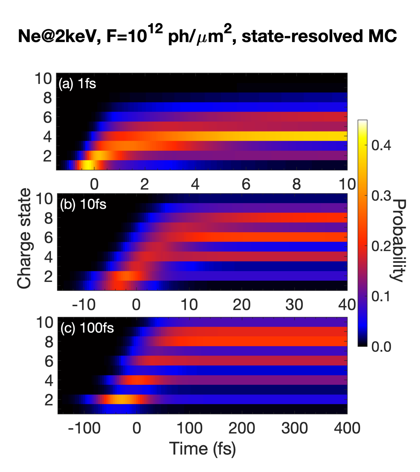


We employ the state-resolved Monte Carlo implementation to examine the time evolution of CSDs and spectra for different pulse durations. We choose pulse durations of 1 fs, 10 fs, and 100 fs FWHM, covering the range of typical pulse durations for current XFEL facilities Pellegrini et al. 2016; Prat et al. 2020; Emma et al. 2010; Ishikawa et al. 2012; Kang et al. 2017; Decking et al. 2020. We consider Ne at a photon energy of 2000 eV and a fluence of , so that in principle all electrons can be ionized via x-ray sequential multiphoton ionization, i.e., a repeated sequence of one-photon ionization and inner-shell relaxation events. In this case, no resonant excitation is involved in the ionization dynamics.
IV.1 Time evolution of charge-state distribution
Figure 6 presents the Ne CSDs as a function of time for pulse durations of (a) 1 fs, (b) 10 fs, and (c) 100 fs FWHM. The temporal peak is located at =0 fs. For clarity, the population of neutral Ne is not included. Note that the sum of charge populations, including the neutral atom, is unity at every time step. The charge distribution building up looks discrete, which indicates that the populations of odd charges are much smaller than those of even charges. This is a consequence of the fact that Auger-Meitner decay follows inner-shell photoionization, when the pulse duration is sufficiently longer than the Auger-Meitner lifetime. One can see that the time-dependent CSD is shifted to lower charges for a shorter pulse duration. For a short pulse duration (1 fs), the CSD peaks around and highly charged ions are barely found as shown in Fig. 6(a). It can be clearly seen that the charged ions are formed sequentially as time goes by, especially near the peak of the pulse. For a long pulse duration (100 fs), however, the distribution becomes broader with a less pronounced peak at as shown in Fig. 6(c). These observations are all indicative of frustrated absorption Hoener et al. 2010 or intensity-induced x-ray transparency Young et al. 2010. The degree of ionization is reduced for shorter pulse duration (i.e., higher intensity) because photoionization defeats Auger-Meitner decay as the intensity increases. This has two consequences. First, a double-core-hole state is formed and, thus, the photoionization cross section is reduced (it is zero for ). In Fig. 7(a), the mean number of photoionization events is depicted as a function of time for the three pulse durations. It may be seen that the photoionization number decreases as the pulse duration becomes shorter. At the same time, the suppression of ionization is also caused by the reduction of the number of Auger-Meitner decays, depicted in Fig. 7(b). These two mechanisms are responsible for the decreased mean charge [Fig. 7(c)] as the pulse is decreased.
Another interesting observation here is that most changes in the time-dependent CSD take place within a time interval of FWHM. However, the shorter the pulse, the more extended is the time interval needed to reach the final charge, because the Auger-Meitner lifetime is often tens of fs (see more details in Sec. IV.2). In Figs. 7(b) and 7(c), the 1-fs curve is not converged to the temporally asymptotic mean value even at FWHM, in contrast to the longer pulse durations. Therefore, in Fig. 6(a), a longer time interval is considered for the 1-fs result.
IV.2 Time-resolved electron and photon spectra
In order to complete our understanding of the x-ray multiphoton ionization dynamics, we calculate time-resolved photoelectron (Fig. 8), Auger-Meitner electron (Fig. 9), and fluorescence spectra (Fig. 10) for all three pulse durations. For all figures, the vertical axis is the time, using FWHM bins, while the horizontal axis is the electron kinetic energy (Figs. 8 and 9) or the photon energy (Fig. 10), using 2-eV bins. Note that all the spectra showcase the number of emitted electrons or photons in a time interval relative to the pulse duration since the time binning is adapted for each pulse duration.
Let us start with the time-resolved photoelectron spectra in Fig. 8. The photoelectron spectra can be grouped according to the peaks belonging to the ionization of Neq+ in a possible configuration dominantly for even charges or dominantly for odd charges (with ). Note that the former leads to the formation of single-core-hole states, while double-core-hole states are produced via the latter. It is apparent from the spectra that lines corresponding to low odd charges (Ne1+ and Ne3+) emerge more with shorter pulse duration in Fig. 8(a). The increased number of outer-shell ionizations of lowly charged ions can be observed in Fig. 8(b). On the other hand, the lines corresponding to the photoionization of highly charged ions appear more for longer pulse durations as shown in Figs. 8(c) and 8(e), which is consistent with the observation in Fig. 6.
Figure 9 shows the time-resolved Auger-Meitner spectra. For long pulse durations, Auger-Meitner decay immediately follows inner-shell ionization and many lines appear in the spectrum as shown in Fig. 9(c). Here, immediately is meant relative to the pulse duration, i.e., when the Auger-Meitner lifetime is sufficiently short in comparison to both the pulse duration and the inverse of the resulting inner-shell photoionization rate, so that Auger-Meitner decay can beat further photoionization. When several Auger-Meitner decays are possible for an initial ion state, lines for more probable processes appear a bit earlier in time. When the pulse duration is decreased, however, Auger-Meitner decay that takes place on longer time scales than the short pulse duration barely occurs during the pulse. Consequently, the number of processes per time bin is reduced, resulting in weaker lines, covering a longer time range, in Figs. 9(a) and 9(b). This reduction of Auger-Meitner decays suppresses refilling of the shell and, thus, further inner-shell photoabsorption, which is one of the mechanisms underlying frustrated absorption as discussed in the previous section. Note that in our state-resolved calculation the time scales for Auger-Meitner decay for Ne ions are in the range from 818 as (Ne2+ ) to 46 fs (Ne7+ ). Thus, most Auger-Meitner decays still take place within 10 fs, as shown in Fig. 9(b). Yet another interesting point is that the decay of the double-core-hole state of Ne2+, i.e., peak (iii), is clearly visible for 1 fs and 10 fs, but is almost absent for 100 fs. This hypersatellite line is located at the highest energy and is well separated from other lines, which provided direct evidence of double-core-hole formation Young et al. 2010; Southworth et al. 2003; Goldsztejn et al. 2016. Decays of other double-core-hole states, with lower energies than peak (iii), can also be observed mainly for short pulse durations.
Finally, we turn to the fluorescence spectra for inner-shell relaxation via transition as shown in Fig. 10. We do not show the fluorescences spectra that are mainly generated long after the pulse on time scales up to ns. For the fluorescence, we can make very similar observations as for the Auger-Meitner spectra, even though Auger-Meitner decay is much more dominant. However, due to lower fluorescence rates in comparison with Auger-Meitner rates, relaxation of highly charged ions via fluorescence takes place on relatively longer time scales even beyond that shown in Fig. 10. Interestingly, single-core-hole and double-core-hole spectra for Ne ions are well separated and ordered by charge, i.e., the higher the charge state, the higher the photon energy for a fixed number of core electrons. (An analogous effect was observed in XFEL experiments on warm dense aluminum Vinko et al. 2012.) The – fluorescence energy is given by , where the initial state has one or two holes and the final state has one hole less than . When has a double vacancy, contains a strong Coulomb repulsion penalty because the two holes are spatially close to each other. Thus, the fluorescence lines from double-core-hole states are higher than those from single-core-hole states corresponding to the same charge state. As the charge state increases, both and increase, but the increase is less for than because in state there is more screening by electrons than in state . Consequently, the fluorescence energy gets larger for higher charge states, which are generated at later times. All these features are demonstrated in the time-dependent fluorescence spectra: In each panel of Fig. 10, there are two groups of transition lines—associated with single- and double-core-hole states, respectively—that move toward higher energies with increasing time.
V Conclusion
In this paper, we have presented an implementation of state-resolved Monte Carlo calculations for describing x-ray multiphoton ionization dynamics. Our implementation in the xatom toolkit employs an improved electronic-structure calculation that is based on first-order many-body perturbation theory. We have compared the new state-resolved and the original configuration-based Monte Carlo calculations for neon at three different photon energies, including a resonant case. The differences in the CSD are negligible when resonances do not matter. Therefore, in these cases the original configuration-based version of xatom already produces quite good results as demonstrated in former studies Doumy et al. 2011; Rudek et al. 2012; Rudek et al. 2018; Rudek et al. 2013; Motomura et al. 2013; Fukuzawa et al. 2013. However, resonant excitations and spectral informations profit from the improved first-order-corrected transition energies in the new implementation. Our results have demonstrated that CSD for the resonance case and calculated electron and photon spectra are improved by using state-resolved ionization dynamics calculations. Employing the state-resolved Monte Carlo implementation, we have investigated CSDs and spectra of neon atoms at a photon energy of 2000 eV for three different XFEL pulse durations. In addition to asymptotic quantities, we have computed time-resolved CSDs and spectra, which highlight the mechanisms through which different pulse durations affect the asymptotic observables. In our example, frustrated absorption clearly manifests itself in the time-resolved spectra as the pulse duration gets shorter. Particularly, it is the dynamical interplay between the suppression of Auger-Meitner decay and the suppression of inner-shell photoabsorption that lies at the heart of frustrated absorption—not the suppression of photoabsorption alone.
We conclude with an outlook. An important next step could be to employ our state-resolved Monte Carlo implementation to explore the orbital alignment of the ions Budewig et al. 2022; Gryzlova et al. 2022 produced during the x-ray multiphoton ionization dynamics. Another promising perspective for further developments is to compare our results on time-dependent quantities with experimental measurements. Experimental methods that may allow such measurements could be attosecond transient absorption spectroscopy Goulielmakis et al. 2010; Wang et al. 2010 and attosecond streaking measurements Itatani et al. 2002; Hentschel et al. 2001; Krausz and Ivanov 2009. These methods have already been employed to investigate ionization dynamics under conditions in which only a few processes were involved Drescher et al. 2002; Schultze et al. 2010. Probing dynamics during x-ray multiphoton ionization may be experimentally challenging due to a wide variety of involved charge states and emitted photo- and Auger-Meitner electrons that are not always well separated, neither in time nor in energy.
VI Acknowledgements
We acknowledge the support by DASHH (Data Science in Hamburg - HELMHOLTZ Graduate School for the Structure of Matter) with the Grant-No. HIDSS-0002.
Appendix A Physical processes and transition energies
| label | process | (eV) | (eV) |
|---|---|---|---|
| (i) | Ne, | 880 () | 857 |
| (ii) | Ne2+, | 935 () | 912 |
| (iii) | Ne1+, | 1001 () | 952 |
| (iv) | Ne4+, | 1006 () | 983 |
| (v) | Ne4+, | 1010 () | 986 |
| (vi) | Ne3+, | 1070 () | 1020 |
| (vii) | Ne, | 49 () | 43 |
| (viii) | Ne, | 20 () | 20 |
| (ix) | Ne1+, | 72 () | 64 |
| (x) | Ne1+, | 66 () | 64 |
| 77 () | – |
| label | process | (eV) | (eV) |
|---|---|---|---|
| (i) | Ne1+, | 801() | 860 |
| 795 () | – | ||
| (ii) | Ne1+, | 764 () | 838 |
| 777 () | – | ||
| (iii) | Ne2+, | 869 () | 875 |
| 863 () | – | ||
| (iv) | Ne2+, | 833 () | 856 |
| (v) | Ne3+, | 764 () | 820 |
| 758 () | – | ||
| (vi) | Ne3+, | 733 () | 800 |
| 729 () | – | ||
| (vii) | Ne4+, | 826 () | 830 |
| (viii) | Ne7+, | 673 () | 717 |
| (ix) | Ne7+, | 654 () | 706 |
| (x) | Ne5+, | – | 788 |
| (xi) | Ne6+, | 690 () | 741 () |
| 690 () | 739 () | ||
| – | 737 () | ||
| (xii) | Ne6+, | 119 () | 125 |
| 14 () | 13 | ||
| (xiii) | Ne7+, | 43 () | 44 () |
| 51 () | 119 () | ||
| – | 131 () | ||
| – | 138 () |
| label | process | (eV) | (eV) |
|---|---|---|---|
| (i) | Ne1+, | 834 () | 906 |
| (ii) | Ne8+, | 919 () | 972 |
| (iii) | Ne8+, | 10 () | 11 |
| 7 () | – | ||
| (iv) | Ne9+, | 1020 () | 1020 |
| (v) | Ne7+, | 916 () | – |
| (vi) | Ne7+, | 140 () | 143 () |
| 183 () | 188 () | ||
| 203 () | 210 () | ||
| 214 () | 222 () | ||
| 220 () | 230 () |
| process | (eV) | (Mb) | (eV) | (Mb) | |
| Ne3+, | 4 | 1043–1059 | – | – | |
| 5 | 1050–1065 | – | – | ||
| Ne5+, | 3 | – | – | 1043 | |
| Ne5+, | 4 | 1052–1054 | 1031 | ||
| Ne6+, | 4 | 1040–1053 | – | – | |
| 5 | 1056–1070 | 1041 | |||
| 6 | 1065–1069 | 1050 | |||
| 7 | – | – | 1055 | ||
| Ne7+, | 3 | 1036–1046 | – | – | |
| 4 | – | – | 1063 | ||
| Ne7+, | 3 | 1064–1067 | 1047 | ||
| 4 | 1067–1070 | 1056 | |||
| 5 | 1070 | 1061 | |||
| 6 | 1070 | 1063 | |||
| 7 | 1070 | 1064 |
References
- Emma et al. (2010) P. Emma, R. Akre, J. Arthur, R. Bionta, C. Bostedt, J. Bozek, A. Brachmann, P. Bucksbaum, R. Coffee, F.-J. Decker, et al., First lasing and operation of an ångstrom-wavelength free-electron laser, Nat. Photon. 4, 641–647 (2010).
- Ishikawa et al. (2012) T. Ishikawa, H. Aoyagi, T. Asaka, Y. Asano, N. Azumi, T. Bizen, H. Ego, K. Fukami, T. Fukui, Y. Furukawa, et al., A compact x-ray free-electron laser emitting in the sub-ångström region, Nat. Photon. 6, 540–544 (2012).
- Decking et al. (2020) W. Decking, S. Abeghyan, P. Abramian, A. Abramsky, A. Aguirre, C. Albrecht, P. Alou, M. Altarelli, P. Altmann, K. Amyan, et al., A MHz-repetition-rate hard x-ray free-electron laser driven by a superconducting linear accelerator, Nat. Photon. 14, 391–397 (2020).
- Kang et al. (2017) H.-S. Kang, C.-K. Min, H. Heo, C. Kim, H. Yang, G. Kim, I. Nam, S. Y. Baek, H.-J. Choi, G. Mun, et al., Hard x-ray free-electron laser with femtosecond-scale timing jitter, Nat. Photon. 11, 708–713 (2017).
- Prat et al. (2020) E. Prat, Abela, M. R., Aiba, et al., A compact and cost-effective hard x-ray free-electron laser driven by a high-brightness and low-energy electron beam, Nat. Photon. 14, 748–756 (2020).
- Pellegrini et al. (2016) C. Pellegrini, A. Marinelli, and S. Reiche, The physics of x-ray free-electron lasers, Rev. Mod. Phys. 88, 015006 (2016).
- Santra and Young (2016) R. Santra and L. Young, in Synchrotron Light Sources and Free-Electron Lasers, edited by E. J. Jaeschke, S. Khan, J. R. Schneider, and J. B. Hastings (Springer International Publishing, Switzerland, 2016), pp. 1233–1260.
- Young et al. (2010) L. Young, E. P. Kanter, B. Krässig, Y. Li, A. M. March, S. T. Pratt, R. Santra, S. H. Southworth, N. Rohringer, L. F. DiMauro, et al., Femtosecond electronic response of atoms to ultra-intense x-rays, Nature 466, 56–61 (2010).
- Fukuzawa et al. (2013) H. Fukuzawa, S.-K. Son, K. Motomura, S. Mondal, K. Nagaya, S. Wada, X.-J. Liu, R. Feifel, T. Tachibana, Y. Ito, et al., Deep inner-shell multiphoton ionization by intense x-ray free-electron laser pulses, Phys. Rev. Lett. 110, 173005 (2013).
- Rudek et al. (2012) B. Rudek, S.-K. Son, L. Foucar, S. W. Epp, B. Erk, R. Hartmann, M. Adolph, R. Andritschke, A. Aquila, N. Berrah, et al., Ultra-efficient ionization of heavy atoms by intense x-ray free-electron laser pulses, Nat. Photon. 6, 858–865 (2012).
- Rudek et al. (2018) B. Rudek, K. Toyota, L. Foucar, B. Erk, R. Boll, C. Bomme, J. Correa, S. Carron, S. Boutet, G. J. Williams, et al., Relativistic and resonant effects in the ionization of heavy atoms by ultra-intense hard x-rays, Nat. Commun. 9, 4200 (2018).
- Rudenko et al. (2017) A. Rudenko, L. Inhester, K. Hanasaki, X. Li, S. J. Robatjazi, B. Erk, R. Boll, K. Toyota, Y. Hao, O. Vendrell, et al., Femtosecond response of polyatomic molecules to ultra-intense hard x-rays, Nature 546, 129–132 (2017).
- Rohringer and Santra (2007) N. Rohringer and R. Santra, X-ray nonlinear optical processes using a self-amplified spontaneous emission free-electron laser, Phys. Rev. A 76, 033416 (2007).
- Makris et al. (2009) M. G. Makris, P. Lambropoulos, and A. Mihelič, Theory of multiphoton multielectron ionization of xenon under strong 93-eV radiation, Phys. Rev. Lett. 102, 033002 (2009).
- Doumy et al. (2011) G. Doumy, C. Roedig, S.-K. Son, C. I. Blaga, A. D. DiChiara, R. Santra, N. Berrah, C. Bostedt, J. D. Bozek, P. H. Bucksbaum, et al., Nonlinear Atomic Response to Intense Ultrashort X Rays, Phys. Rev. Lett. 106, 083002 (2011).
- Xiang et al. (2012) W. Xiang, C. Gao, Y. Fu, J. Zeng, and J. Yuan, Inner-shell resonant absorption effects on evolution dynamics of the charge state distribution in a neon atom interacting with ultraintense x-ray pulses, Phys. Rev. A 86, 061401(R) (2012).
- Rudek et al. (2013) B. Rudek, D. Rolles, S.-K. Son, L. Foucar, B. Erk, S. Epp, R. Boll, D. Anielski, C. Bostedt, S. Schorb, et al., Resonance-enhanced multiple ionization of krypton at an x-ray free-electron laser, Phys. Rev. A 87, 023413 (2013).
- Motomura et al. (2013) K. Motomura, H. Fukuzawa, S.-K. Son, S. Mondal, T. Tachibana, Y. Ito, M. Kimura, K. Nagaya, T. Sakai, K. Matsunami, et al., Sequential multiphoton multiple ionization of atomic argon and xenon irradiated by x-ray free-electron laser pulses from SACLA, J. Phys. B: At. Mol. Opt. Phys. 46, 164024 (2013).
- Berrah et al. (2019) N. Berrah, A. Sanchez-Gonzalez, Z. Jurek, R. Obaid, H. Xiong, R. J. Squibb, T. Osipov, A. Lutman, L. Fang, T. Barillot, et al., Femtosecond-resolved observation of the fragmentation of buckminsterfullerene following x-ray multiphoton ionization, Nat. Phys. 15, 1279–1283 (2019).
- Murphy et al. (2014) B. F. Murphy, T. Osipov, Z. Jurek, L. Fang, S.-K. Son, M. Mucke, J. H. D. Eland, V. Zhaunerchyk, R. Feifel, L. Avaldi, et al., Femtosecond x-ray-induced explosion of at extreme intensity, Nat. Commun. 5, 4281 (2014).
- Hoener et al. (2010) M. Hoener, L. Fang, O. Kornilov, O. Gessner, S. T. Pratt, M. Gühr, E. P. Kanter, C. Blaga, C. Bostedt, J. D. Bozek, et al., Ultraintense x-ray induced ionization, dissociation, and frustrated absorption in molecular nitrogen, Phys. Rev. Lett. 104, 253002 (2010).
- Toyota et al. (2017) K. Toyota, S.-K. Son, and R. Santra, Interplay between relativistic energy corrections and resonant excitations in x-ray multiphoton ionization dynamics of Xe atoms, Phys. Rev. A 95, 043412 (2017).
- Son et al. (2020) S.-K. Son, R. Boll, and R. Santra, Breakdown of frustrated absorption in x-ray sequential multiphoton ionization, Phys. Rev. Research 2, 023053 (2020).
- Ho et al. (2015) P. J. Ho, E. P. Kanter, and L. Young, Resonance-mediated atomic ionization dynamics induced by ultraintense x-ray pulses, Phys. Rev. A 92, 063430 (2015).
- Ho et al. (2014) P. J. Ho, C. Bostedt, S. Schorb, and L. Young, Theoretical tracking of resonance-enhanced multiple ionization pathways in x-ray free-electron laser pulses, Phys. Rev. Lett. 113, 253001 (2014).
- Mazza et al. (2020) T. Mazza, M. Ilchen, M. D. Kiselev, E. V. Gryzlova, T. M. Baumann, R. Boll, A. De Fanis, P. Grychtol, J. Montaño, V. Music, et al., Mapping resonance structures in transient core-ionized atoms, Phys. Rev. X 10, 041056 (2020).
- Son and Santra (2012) S.-K. Son and R. Santra, Monte Carlo calculation of ion, electron, and photon spectra of xenon atoms in x-ray free-electron laser pulses, Phys. Rev. A 85, 063415 (2012).
- Schäfer et al. (2018) J. M. Schäfer, L. Inhester, S.-K. Son, R. F. Fink, and R. Santra, Electron and fluorescence spectra of a water molecule irradiated by an x-ray free-electron laser pulse, Phys. Rev. A 97, 053415 (2018).
- Buth et al. (2018) C. Buth, R. Beerwerth, R. Obaid, N. Berrah, L. S. Cederbaum, and S. Fritzsche, Neon in ultrashort and intense x-rays from free electron lasers, J. Phys. B: At. Mol. Opt. Phys. 51, 055602 (2018).
- Lorenz et al. (2012) U. Lorenz, N. M. Kabachnik, E. Weckert, and I. A. Vartanyants, Impact of ultrafast electronic damage in single-particle x-ray imaging experiments, Phys. Rev. E 86, 051911 (2012).
- Quiney and Nugent (2011) H. M. Quiney and K. A. Nugent, Biomolecular imaging and electronic damage using x-ray free-electron lasers, Nat. Phys. 7, 142–146 (2011).
- Son et al. (2011) S.-K. Son, L. Young, and R. Santra, Impact of hollow-atom formation on coherent x-ray scattering at high intensity, Phys. Rev. A 83, 033402 (2011).
- Chapman et al. (2011) H. N. Chapman, P. Fromme, A. Barty, T. A. White, R. A. Kirian, A. Aquila, M. S. Hunter, J. Schulz, D. P. DePonte, U. Weierstall, et al., Femtosecond x-ray protein nanocrystallography, Nature 470, 73–77 (2011).
- Coe and Fromme (2016) J. Coe and P. Fromme, Serial femtosecond crystallography opens new avenues for structural biology, Protein Pept Lett. 23, 255–272 (2016).
- Sobolev et al. (2020) E. Sobolev, S. Zolotarev, K. Giewekemeyer, J. Bielecki, K. Okamoto, H. Reddy, J. Andreasson, K. Ayyer, I. Barák, S. Bari, et al., Megahertz single-particle imaging at the European XFEL, Commun. Phys. 3, 97 (2020).
- Seibert et al. (2011) M. M. Seibert, T. Ekeberg, F. R. N. C. Maia, M. Svenda, J. Andreasson, O. Jönsson, D. Odić, B. Iwan, A. Rocker, D. Westphal, et al., Single mimivirus particles intercepted and imaged with an x-ray laser, Nature 470, 78–81 (2011).
- Nass (2019) K. Nass, Radiation damage in protein crystallography at x-ray free-electron lasers, Acta Cryst. D 75, 211–218 (2019).
- Ciricosta et al. (2011) O. Ciricosta, H.-K. Chung, R. W. Lee, and J. S. Wark, Simulations of neon irradiated by intense x-ray laser radiation, High Energy Density Phys. 7, 111–116 (2011).
- Buth et al. (2012) C. Buth, J.-C. Liu, M. H. Chen, J. P. Cryan, L. Fang, J. M. Glownia, M. Hoener, R. N. Coffee, and N. Berrah, Ultrafast absorption of intense x rays by nitrogen molecules, J. Chem. Phys. 136, 214310 (2012).
- Liu et al. (2016) J.-C. Liu, N. Berrah, L. S. Cederbaum, J. P. Cryan, J. M. Glownia, K. J. Schafer, and C. Buth, Rate equations for nitrogen molecules in ultrashort and intense x-ray pulses, J. Phys. B: At. Mol. Opt. Phys. 49, 075602 (2016).
- Jurek et al. (2016) Z. Jurek, S.-K. Son, B. Ziaja, and R. Santra, XMDYN and XATOM: Versatile simulation tools for quantitative modeling of X-ray free-electron laser induced dynamics of matter, J. Appl. Cryst. 49, 1048–1056 (2016).
- (42) S.-K. Son, K. Toyota, O. Geffert, J. M. Slowik, and R. Santra, xatom-an integrated toolkit for x-ray and atomic physics, CFEL, DESY, Hamburg, Germany, 2016, Rev. 3544.
- Budewig et al. (2022) L. Budewig, S.-K. Son, and R. Santra, Theoretical investigation of orbital alignment of x-ray-ionized atoms in exotic electronic configurations, Phys. Rev. A 105, 033111 (2022).
- Slater (1951) J. C. Slater, A Simplification of the Hartree-Fock Method, Phys. Rev. 81, 385–390 (1951).
- Griffiths (2017) D. J. Griffiths, Introduction to Quantum Mechanics; 2nd edition (Cambridge University Press, Cambridge, 2017).
- Sakurai and Napolitano (2014) J. J. Sakurai and J. J. Napolitano, Modern Quantum Mechanics: Pearson New International Edition (Pearson Education, Harlow, 2014).
- Gottfried and Yan (2003) K. Gottfried and T. Yan, Quantum Mechanics: Fundamentals (Springer, New York, 2003).
- Racah (1942) G. Racah, Theory of Complex Spectra. II, Phys. Rev. 62, 438–462 (1942).
- Judd (1963) B. R. Judd, Operator Techniques in Atomic Spectroscopy (McGraw-Hill Book Company, New York, 1963).
- Hertel and Schulz (2015) I. V. Hertel and K. P. Schulz, Atoms, Molecules and Optical Physics 1 (Springer, Berlin, 2015).
- Santra (2009) R. Santra, Concepts in x-ray physics, J. Phys. B: At. Mol. Opt. Phys. 42, 023001 (2009).
- Sytcheva et al. (2012) A. Sytcheva, S. Pabst, S.-K. Son, and R. Santra, Enhanced nonlinear response of to intense ultrafast x rays, Phys. Rev. A 85, 023414 (2012).
- Tilley et al. (2015) M. Tilley, A. Karamatskou, and R. Santra, Wave-packet propagation based calculation of above-threshold ionization in the x-ray regime, J. Phys. B: At. Mol. Opt. Phys. 48, 124001 (2015).
- Schneider et al. (2002) T. Schneider, P. L. Chocian, and J.-M. Rost, Separation and identification of dominant mechanisms in double photoionization, Phys. Rev. Lett. 89, 073002 (2002).
- Kolorenč et al. (2016) P. Kolorenč, V. Averbukh, R. Feifel, and J. Eland, Collective relaxation processes in atoms, molecules and clusters, J. Phys. B: At. Mol. Opt. Phys. 49, 082001 (2016).
- Saito and Suzuki (1994) N. Saito and I. H. Suzuki, Shake-off processes in photoionization and auger transition for rare gases irradiated by soft x-rays, Phys. Scr. 49, 80–85 (1994).
- Rohringer and Santra (2008) N. Rohringer and R. Santra, Resonant auger effect at high x-ray intensity, Phys. Rev. A 77, 053404 (2008).
- Rohringer and Santra (2012) N. Rohringer and R. Santra, Strongly driven resonant auger effect treated by an open-quantum-system approach, Phys. Rev. A 86, 043434 (2012).
- Kanter et al. (2011) E. P. Kanter, B. Krässig, Y. Li, A. M. March, P. Ho, N. Rohringer, R. Santra, S. H. Southworth, L. F. DiMauro, G. Doumy, et al., Unveiling and driving hidden resonances with high-fluence, high-intensity x-ray pulses, Phys. Rev. Lett. 107, 233001 (2011).
- Li et al. (2016) Y. Li, C. Gao, W. Dong, J. Zeng, Z. Zhao, and J. Yuan, Coherence and resonance effects in the ultra-intense laser-induced ultrafast response of complex atoms, Sci. Rep. 6, 18529 (2016).
- Nandi et al. (2022) S. Nandi, E. Olofsson, M. Bertolino, S. Carlström, F. Zapata, D. Busto, C. Callegari, M. D. Fraia, P. Eng-Johnsson, R. Feifel, et al., Observation of Rabi dynamics with a short-wavelength free-electron laser, Nature 608, 488–493 (2022).
- Cavaletto et al. (2012) S. M. Cavaletto, C. Buth, Z. Harman, E. P. Kanter, S. H. Southworth, L. Young, and C. H. Keitel, Resonance fluorescence in ultrafast and intense x-ray free-electron-laser pulses, Phys. Rev. A. 86, 033402 (2012).
- Toyota et al. (2019) K. Toyota, Z. Jurek, S.-K. Son, H. Fukuzawa, K. Ueda, N. Berrah, B. Rudek, D. Rolles, A. Rudenko, and R. Santra, xcalib: a focal spot calibrator for intense x-ray free-electron laser pulses based on the charge state distributions of light atoms, J. Synchrotron Rad. 26, 1017–1030 (2019).
- Efron and Tibshirani (1994) B. Efron and R. J. Tibshirani, An introduction to the bootstrap (Chapman and Hall/CRC, Philadelphia, PA, 1994).
- Southworth et al. (2003) S. H. Southworth, E. P. Kanter, B. Krässig, L. Young, G. B. Armen, J. C. Levin, D. L. Ederer, and M. H. Chen, Double -shell photoionization of neon, Phys. Rev. A 67, 062712 (2003).
- Goldsztejn et al. (2016) G. Goldsztejn, T. Marchenko, R. Püttner, L. Journel, R. Guillemin, S. Carniato, P. Selles, O. Travnikova, D. Céolin, A. F. Lago, et al., Double-core-hole states in neon: Lifetime, post-collision interaction, and spectral assignment, Phys. Rev. Lett. 117, 133001 (2016).
- Vinko et al. (2012) S. M. Vinko, O. Ciricosta, B. I. Cho, K. Engelhorn, H.-K. Chung, C. R. D. Brown, T. Burian, J. Chalupský, R. W. Falcone, C. Graves, et al., Creation and diagnosis of a solid-density plasma with an x-ray free-electron laser, Nature 482, 59–62 (2012).
- Gryzlova et al. (2022) E. V. Gryzlova, A. N. Grum-Grzhimailo, M. D. Kiselev, and M. M. Popova, Evolution of the ionic polarization in multiple sequential ionization: general equations and an illustrative example (2022).
- Goulielmakis et al. (2010) E. Goulielmakis, Z.-H. Loh, A. Wirth, R. Santra, N. Rohringer, V. S. Yakovlev, S. Zherebtsov, T. Pfeifer, A. M. Azzeer, M. F. Kling, et al., Real-time observation of valence electron motion, Nature 466, 739–744 (2010).
- Wang et al. (2010) H. Wang, M. Chini, S. Chen, C.-H. Zhang, F. He, Y. Cheng, Y. Wu, U. Thumm, and Z. Chang, Attosecond time-resolved autoionization of argon, Phys. Rev. Lett. 105, 143002 (2010).
- Itatani et al. (2002) J. Itatani, F. Quere, G. L. Yudin, M. Y. Ivanov, F. Krausz, and P. B. Corkum, Attosecond streak camera, Phys. Rev. Lett. 88, 173903 (2002).
- Hentschel et al. (2001) M. Hentschel, R. Kienberger, C. Spielmann, G. A. Reider, N. Milosevic, T. Brabec, P. Corkum, U. Heinzmann, M. Drescher, and F. Krausz, Attosecond metrology, Nature 414, 509–513 (2001).
- Krausz and Ivanov (2009) F. Krausz and M. Ivanov, Attosecond physics, Rev. Mod. Phys. 81, 163–234 (2009).
- Drescher et al. (2002) M. Drescher, M. Hentschel, R. Kienberger, M. Uliberacker, V. Yakovlev, A. Scrinzi, T. Westerwalbesloh, U. Kleineberg, U. Heinzmann, and F. Krausz, Time-resolved atomic inner-shell spectroscopy, Nature 419, 803–807 (2002).
- Schultze et al. (2010) M. Schultze, M. Fiess, N. Karpowicz, J. Ggnon, M. Korbman, M. Hofstetter, S. Neppl, A. L. Cavalieri, Y. Komninos, T. Mercouris, et al., Delay in photoemission, Science 328, 1658–1662 (2010).