Differential Dynamic Microscopy can be applied to Differential Interference Contrast images despite shadowing effects

A DIC image is formed by pairs of closely spaced polarised beams [10], with their separation denoted as the ‘shear’, which is typically similar to optical resolution in the focal plane. The beams are then recombined and analysed, converting a mutual phase difference into an intensity difference in the resulting image.

A sketch of a DIC microscope with de-Sénarmont compensation and its workings is given in Figure 2. Starting from a bright-field transmission microscope in Köhler illumination, the illumination is linearly polarised at $45\degree+\theta$, and then transmitted through a quarter-wave plate with the fast axis at 45°, resulting in electric field components $E_{x}$ and $E_{y}$ in $x$ and $y$ direction, respectively, of equal amplitude and a relative phase shift of $\psi=2\theta$. A Wollaston prism splits the propagation direction of $E_{x}$ and $E_{y}$ in the condenser back focal plane, resulting in a relative displacement of the corresponding focal points at the sample by the shear $\mathbf{s}$ along the $x$ direction. The fields are probing the sample properties accordingly at two positions displaced by $\mathbf{s}$, and acquiring a spatially dependent phase difference $\delta(\mathbf{r})$, with the in-plane sample position $\mathbf{r}=(x,y)$. After transmission through the sample, the two fields are recombined in direction at the back focal plane of the objective by a Wollaston prism matched to the first one (a Nomarski prism can be used instead, which allows to have the effective recombination position displaced from the prism and thus to position the prism at a accessible place in the beam path after the objective). A second polariser, called analyser, orientated at -45°, orthogonal to the first one, is projecting the recombined fields along its axis to provide an intensity interference. The resulting transmitted intensity $I_{\rm t}$ has a dependence on the phase shift $\delta(\mathbf{r})$ given by

with the excitation intensity $I_{\rm e}$, the position in the sample plane $\mathbf{r}$, the phase offset $\psi$, and the difference $\delta(\mathbf{r})$ of the optical phase shift $\phi$ for the two beams that pass through the sample in two adjacent points separated by the shear vector $\mathbf{s}$.

Adjusting the phase offset $\psi$, the contrast can be changed from a dark-field type at $\psi=0$, where the intensity is proportional to $\delta^{2}(\mathbf{r})$, to a bright field image modulated by a term linear with the phase shift, with the largest linear range for $\psi=90\degree$, for a polariser angle of $\theta=45\degree$.

More details on the theory of DIC can be found in Ref. [15] for two-dimensional samples, in Ref. [16] for three-dimensional samples, and a fully vectorial treatment of the fields is given in Ref. [17].

As test standard for the DDM analysis, polystyrene (PS) beads, having a nominal radius of 100 nm with less than 3% coefficient of variance (cv), were purchased (Alpha Nanotech Colloidal PS Beads NP-PA07CPSX78). These PS beads were dispersed in 30% v/v glycerol/water mixtures to a particle concentration of 0.1 mg/mL, 13 µl were pipetted into a 0.12 mm high and 13 mm diameter chamber made of a Grace Bio-Labs (Bend, US) SecureSeal imaging spacer on a $(76\times 26\times 1)$ mm³ microscope slide (Menzel Gläser). The chamber was then sealed with a ($24\times 24$) mm² #1.5 coverslip (Menzel Gläser), and stored in a 100% humidity environment at 7°C until use.

8 week old CD1 mice were intraperitoneally injected with 5IU pregnant mare’s serum gonadotrophin (PMSG) to induce ovarian follicle development. They were again injected with 10IU human chorionic gonadotrophin (hCG) approximately 48hrs later to induce ovulation. Ovulated mature (MII) eggs were collected from oviducts approximately 15hrs later. All animals were handled according to UK Home Office regulations, and procedures were carried out under a UK Home Office Project License with the approval of Cardiff University Animal Ethics Committee. Live imaging experiments were carried out with mature eggs cultured in HKSOM as described previously [18]. All drops were covered with mineral oil (embryo tested, Sigma) to prevent evaporation.

DIC images were obtained using an inverted Nikon Ti-U microscope as in [19, 13]. Samples were illuminated using a 100 W halogen lamp (Nikon V2-A LL 100 W) followed by a Schott BG40 filter to remove wavelengths above 650 nm (for which the DIC polarisers are not suited) and a Nikon green interference filter (Nikon GIF), to define the wavelength range centred at 550 nm and having a full-width at half maximum (FWHM) of 53 nm. This illumination was then passed through a de-Sénarmont compensator (a rotatable linear polariser and quarter-wave plate, Nikon T-P2 DIC Polariser HT MEN51941) and a Nomarski prism (Nikon N2 DIC module MEH52400 or MEH52500) and focused onto the sample by a condenser (MEL56100) of 0.72 numerical aperture (NA). The shear of the Nikon N2 DIC was measured to be $(238\pm 10)$ nm. The objective used was a $20\times$ 0.75 NA planapochromat (MRD00205). After the objectives, light passes through a suited Nomarski prism (DIC slider MBH76220) and a linear polariser (Nikon Ti-A-E DIC analyser block MEN 51980). Images were detected by a Hamamatsu Orca 285 CCD camera (18,000 electrons full well capacity, 7 electrons read noise, and 4.6 electrons per count, 12 bit digitiser, $1344\times 1024$ pixels, pixel size 6.45 $\mu$m, 192 counts offset). The microscope was adjusted for Köhler illumination, and the field aperture was set to be slightly larger than the imaged sample region.

For the images of colloids, a sequence of $N_{\rm a}$ frames (up to 256) were acquired, with 120 ms exposure time per frame (given by highest stably achievable frame rate), with the lamp intensity adjusted to provide a mean intensity of about 3000 counts (13000 photoelectrons) per pixel. Data for de-Sénarmont polariser angles $\pm\theta$ as well as zero were taken to enable qDIC analysis, for $\theta$ of 15, 30, and 45 degrees. The rotation of the de-Sénarmont polariser was motorized (by a home-built modification) to improve positioning speed and reproducibility. DIC images of the colloids were acquired with a 20 x objective and 1.5 x tubular lens at a polarisation angle of 15°. For DM analysis, a total of 7680 frames were taken at +15° and an average of 256 frames at -15° were used to post process the data.

For the mouse oocyte in Figure 1, DIC images were acquired with 20x objective with 1.5 tubular lens, by a monochrome ORCA285 Hamamatsu CCD camera with 120 ms frame exposure time and a 12.5° polarisation angle in the de-Senarmont DIC illuminator (yielding a 25° phase offset). A motorized stage and z-drive (Prior ProScan III) enabled lateral xy sample movement and axial z focus movement for focusing. For DM analysis, polarisation angle was changed to the opposite side every 30s, during which 256 frames of DIC images were acquired.

Comprehensive descriptions of the DDM technique are available in literature [20], alongside MATLAB/Python codes and datasets [21]. Here, we provide a brief overview of the DDM algorithm.

Consider an image stack $I(\bm{r},t)$ consisting of $N$ digital images that are $L\times W$ pixels long and wide, respectively, taken at regularly spaced times $t\in\{0$, $\Delta t_{\text{min}}$, $2\Delta t_{\text{min}}$ … $(N-1)\Delta t_{\text{min}}\}=T$, where $t_{\text{min}}$ is the time between consecutive frames. Here, $\bm{r}$ denotes the Cartesian location of each pixel. Define the time between any two given frames as $\Delta t$, if $t+\Delta t\in T$. Then define the image difference

Denoting the spatial Fourier transform by $\tilde{\cdot}$, the spatial frequency vector by $\bm{q}=(q_{x},q_{y})$, and the time average by $\langle\cdot\rangle_{t}$, we define the DDM tensor as

where $n$ is the number of frames elapsed during the time lag $\Delta t$. Denoting the complex conjugate by $\cdot^{*}$ and commutative element-wise matrix multiplication (Hadamard product) by $\odot$, the DDM tensor can be expanded and written as [3, 21]

Unless otherwise stated, throughout this work matrix multiplication will be element wise, so we drop the explicit $\odot$ notation. The term

is the real part of the Intermediate Scattering Function (ISF) [21, 20], which is equal to the real part of the Fourier transform of the van Hove function $G(\bm{r},t)$, which counts the expected number of particles $j$ found at the location $\bm{r}$ at time $t$ given a particle $i$ is located at the origin at time $t=0$ [22]. When particles act independently, this can be used to describe the probability density function describing motion of particles in the system (further explanation for this relationship is given in the Supplementary Materials).

Assuming the imaged motion is isotropic and that the images are not spatially heterogeneous, an azimuthal average can be applied to Equation (3) for dimensional reduction and to average over random movement within the image stack. We express this as the contour integral

where $||\cdot||$ is the length of the contour $\Gamma$, and

The azimuthal average of $\mathcal{D}(\bm{q},\Delta t)$ is a matrix, commonly expressed as

where

is a scaling parameter depending on the appearance of particles [3]. In practice, it is necessary to add an additional term $B(\bm{q})$ to Equation (5), which accounts for random noise from the camera [21, 5, 9]. If an analytic form of $f(q,\Delta t)$ is known, we can evaluate $\mathcal{D}(q,\Delta t)$ numerically by iterating Equation (2) over the image stack, and then employ numerical fitting approaches to Equation (5) to determine parameters within $f(q,\Delta t)$. For example, in Brownian motion, it is known that $f(q,\Delta t)$ has the form

where $D$ ($\mu\text{m}^{2}/\text{s}$) is the diffusion coefficient [3, 21, 23]. If we fix $q$ in the DDM matrix, both $A(q)$ and $B(q)$ in Equation (5) become constant, allowing us to first probe the time dependency of $f(q,\Delta t)$, and then fit again to probe the dependency on $q$. Often for diffusion problems [3, 21, 5], this two step approach first numerically fits some $q$ dependent term $\tau_{q}=(q^{2}D)^{-1}$, and then determines $D$ by fitting

In Figure 3, we plot $\mathcal{D}(\bm{q},\Delta t)$ at the smallest time lag available for two different movies of colloidal dispersions; 3(a) comes from bright field images of a colloidal dispersion [21], with concentric rings demonstrating that the underlying process is isotropic [21]. However, 3(b), derived from DIC images of a similar colloidal dispersion, shows an asymmetric ‘kidney bean’ shape, where the highest peaks align along the orientation of the shear $\mathbf{s}$ in the DIC image, and the lowest are orthogonal to it.

Since we know the colloidal dispersion is subject only to isotropic Brownian motion [24], the anisotropy in Figure 3, right, is an artefact of the DIC imaging process. We now derive an expression to characterise and resolve this anisotropy.

A single DIC image can be expressed as the difference between overlapping identical offset images [25], where each polarised beam in the pair generates a different image. For a DIC image stack $I(\bm{r},t)$, there exists image stacks $X(\bm{r},t)$ and $Y(\bm{r},t)$ such that

for a shear $\mathbf{s}=(x_{0},y_{0})$. For some initial time, $t$, and some time displacement $\Delta t$, let $I_{2}=I(\bm{r},t+\Delta t)$ and $I_{1}=I(\bm{r},t)$, with the relation $I_{j}=Y_{j}-X_{j},$ $j\in\{1,2\}$. Hence, $\Delta I=\Delta Y-\Delta X$, and we construct the DDM matrix for the DIC image, denoted $\mathcal{D}_{I}$, as follows;

Comparing to Equation (2), $\mathcal{D}_{Y}\equiv\left\langle\left|\Delta\tilde{Y}\right|^{2}\right\rangle_{t}$ and $\mathcal{D}_{X}\equiv\left\langle\left|\Delta\tilde{X}\right|^{2}\right\rangle_{t}$. In DIC microcopy, shear distances may be as small as 0.2-0.3 $\mu$m [26, 25, 10], which means that this displacement is small relative to the size of the image. Hence, it is unlikely that the sampled dynamics between the image sets will differ significantly, and we conclude that $\mathcal{D}_{Y}\approx\mathcal{D}_{X}$.

By the translation property of the Fourier transform,

and rearranging the definition of the ISF in (4), we may rewrite Equation (6) as

Assuming a sufficiently high signal to noise ratio, such that noise is negligible, Equation (5) defines the DDM tensor on a DIC image stack as

As previously, the next step in the DDM analysis is to apply an azimuthal average. We first simplify our analysis by assuming the underlying motion, and therefore $f(\bm{q},\Delta t)$, is isotropic, for example in the case of swimming bacteria [4] or colloidal dispersions [3].

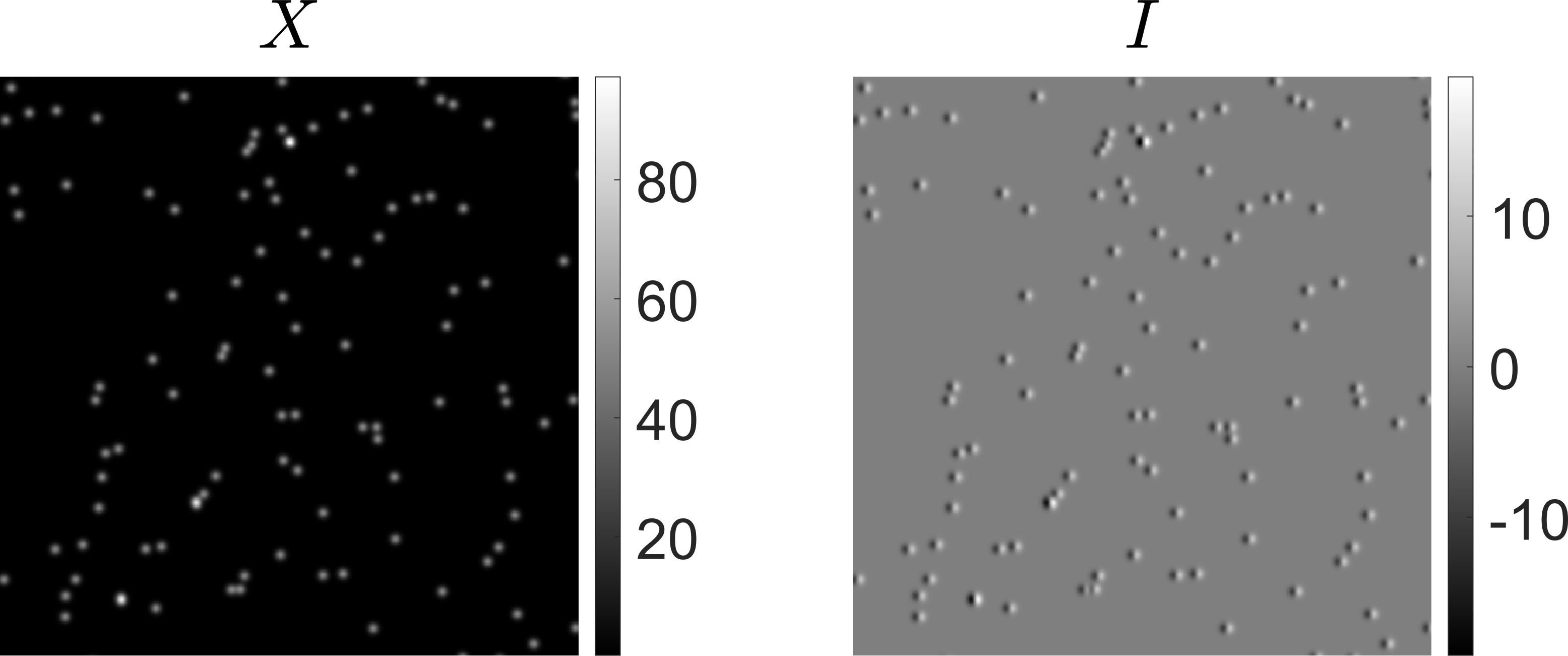
We generate simulations of 150 particles moving inside a 490$\times$490 window, with diffusion coefficient $D=0.5\mu\text{m}^{2}/\text{s}$, where 1 pixel represents 1 $\mu$m, for a duration of 4000 frames at a frequency of $8$ frames per second. From these simulations, we generate the phase image stack $X(\bm{r},t)$ and the corresponding DIC image stack $I(\bm{r},t)$ using a DIC shift of 1 pixel to the right, i.e $\bm{s}=(1,0)$. The first frame of each image stack is visualised in Figure 4 From each image stack, we generate the corresponding DDM matrices $D_{X}$ and $D_{I}$, respectively. More details about the simulations are available in Supplementary Material, and the code is available at https://github.com/OstlerT/DIC_DDM_Ostler.git.

In Figure 5, we demonstrate that the decomposition in Equation (11) holds for all frequencies $q<2\mu\text{m}^{-1}$. For different sets of simulation parameters, the agreement can deteriorate at very high and very low frequencies, but it is standard practice in DDM analysis to restrict fitting to some interval on $q$ away from the lowest available frequencies, where statistical sampling of the radial average is poor, and away from large frequencies where the signal to noise ratio is poor [21]. As such, as long as the relationship holds over the optimal fitting region, we can conclude that the analysis of $\mathcal{D}_{X}$ and $\mathcal{D}_{Y}$ will yield equivalent results.

We now show that the diffusion coefficients generated by fitting $\mathcal{D}_{X}$ and $\mathcal{D}_{I}$ are equivalent. We generate 150 movies of diffusing particles, choosing the diffusion coefficient to be $D=0.5\,\mu\text{m}^{2}/\text{s}$ to remain consistent with literature simulation approaches [8], and perform fitting over the frequency interval $0.3\mu\text{m}^{-1}<q<0.8\,\mu\text{m}^{-1}$. The average diffusion coefficients generated by the simulations of $X$ and $I$ are $\overline{D}_{X}=0.481\pm 0.009\mu\text{m}^{2}/\text{s}$, and $\overline{D}_{I}=0.482\pm 0.010\mu\text{m}^{2}/\text{s}$, respectively, with the distribution of the fitted diffusion coefficients plotted in Figure 6(a). Although a wide spread of fitted diffusion coefficients arises in the simulations, plotting the values $D_{X}-D_{I}$ as a histogram in Figure 6(b) shows the fitting difference is small between $\mathcal{D}_{X}$ and $\mathcal{D}_{I}$. Hence, DIC shadowing has a minimal effect on the fitted diffusion coefficient.

Additionally, we show that DDM is accurate in a single image stack formed of 7680 DIC images of a colloidal dispersion, as described in Section 2.2. The images are $1344\times 1024$ pixels representing a $433.44\times 330.24$ $\mu$m real region (pixel length $322.5$ nm), from which we take a square subset with a side length of $1024$ pixels. The shearing distance is measured to be $238\pm 10$ nm [26], the pixel length is $322.5\,$nm, with a shear angle of $\phi=\pi/4$ and a phase offset of 90^∘. From the corresponding DDM matrix, $\mathcal{D}_{I}$, we fit a diffusion coefficient of $0.676\,\mu\text{m}^{2}/\text{s}$. Comparing this to the Stokes-Einstein relation [3, 21],

the expected diffusion coefficient is $0.667$ $\mu\text{m}^{2}/\text{s}$, where $K_{B}$ is the Boltzmann constant, $T=291.25$K is absolute temperature, $\eta=3.20$ mPa $(\text{s}^{-1})$ is the dynamic viscosity of a $30\%$ glycerol solution, and $r$ the particle radius. Hence, $D$ is comparable to the fitted value. We visualise $\tau_{\mathcal{D}_{I}}$, $A(q)$, $B(q)$ and the fitting regime in Figure 7.

Although we have only shown that our results hold for Brownian motion, the relationship (10) holds for all forms of isotropic motion. However, we cannot make the same claims for anisotropic motion, since the azimuthal average of Equation (8) contains the term

which we cannot evaluate without knowing the exact form of $f(\bm{q},\Delta t)$. For now, we consider directed advection-diffusion, a specific form of anisotropy present in the motivating example of classifying the rate of cytoplasmic movement in oocytes [5].

References

- [1] Jepson A, Arlt J, Statham J, Spilman M, Burton K, Wood T, et al. High-throughput characterisation of bull semen motility using differential dynamic microscopy. PLOS One. 2019;14(4):e0202720.
- [2] Ajduk A, Ilozue T, Windsor S, Yu Y, Seres KB, Bomphrey RJ, et al. Rhythmic actomyosin-driven contractions induced by sperm entry predict mammalian embryo viability. Nat Commun. 2011;2(1).
- [3] Cerbino R, Trappe V. Differential dynamic microscopy: probing wave vector dependent dynamics with a microscope. Phys Rev Lett. 2008;100(18):188102.
- [4] Wilson LG, Martinez VA, Schwarz-Linek J, Tailleur J, Bryant G, Pusey PN, et al. Differential Dynamic Microscopy of Bacterial Motility. Phys Rev Lett. 2011;106(1):018101.
- [5] Drechsler M, Giavazzi F, Cerbino R, Palacios IM. Active diffusion and advection in Drosophila oocytes result from the interplay of actin and microtubules. Nature communications. 2017;8(1):1-11.
- [6] He K, Spannuth M, Conrad JC, Krishnamoorti R. Diffusive dynamics of nanoparticles in aqueous dispersions. Soft Matter. 2012;8(47):11933-8.
- [7] Lu PJ, Giavazzi F, Angelini TE, Zaccarelli E, Jargstorff F, Schofield AB, et al. Characterizing Concentrated, Multiply Scattering, and Actively Driven Fluorescent Systems with Confocal Differential Dynamic Microscopy. Phys Rev Lett. 2012;108(21):218103.
- [8] Bayles AV, Squires TM, Helgeson ME. Dark-field differential dynamic microscopy. Soft Matter. 2016;12(8):2440-52.
- [9] Martinez VA, Besseling R, Croze OA, Tailleur J, Reufer M, Schwarz-Linek J, et al. Differential Dynamic Microscopy: A High-Throughput Method for Characterizing the Motility of Microorganisms. Biophys J. 2012;103(8):1637-47.
- [10] Murphy DB, Davidson MW. Fundamentals of Light Microscopy and Electronic Imaging. John Wiley & Sons, Inc.; 2002.
- [11] Hoffman R, Gross L. Modulation Contrast Microscope. Appl Opt. 1975;14(5):1169.
- [12] Allen R, David G. The Zeiss-Nomarski differential interference equipment for transmitted-light microscopy. Z Wiss Mikrosk. 1969;69(4):193-221.
- [13] Hamilton S, Regan D, Payne L, Langbein W, Borri P. Sizing individual dielectric nanoparticles with quantitative differential interference contrast microscopy. The Analyst. 2022;147(8):1567-80.
- [14] Reufer M, Martinez VA, Schurtenberger P, Poon WCK. Differential Dynamic Microscopy for Anisotropic Colloidal Dynamics. Langmuir. 2012;28(10):4618-24.
- [15] Holmes TJ, Levy WJ. Signal-processing characteristics of differential-interference-contrast microscopy. Appl Opt. 1987;26(18):3929.
- [16] Preza C, Snyder DL, Conchello JA. Theoretical development and experimental evaluation of imaging models for differential-interference-contrast microscopy. J Opt Soc Am A. 1999;16(9):2185-99.
- [17] Munro PRT, Török P. Vectorial, high numerical aperture study of Nomarski’s differential interference contrast microscope. Opt Express. 2005;13(18):6833.
- [18] Wang Y, Pope I, Brennan-Craddock H, Poole E, Langbein W, Borri P, et al. A primary effect of palmitic acid on mouse oocytes is the disruption of the structure of the endoplasmic reticulum. Reproduction. 2022;163(1):45-56.
- [19] Regan K, Wulstein D, Rasmussen H, McGorty R, Robertson-Anderson RM. Bridging the spatiotemporal scales of macromolecular transport in crowded biomimetic systems. Soft Matter. 2019;15(6):1200-9.
- [20] Giavazzi F, Cerbino R. Digital Fourier microscopy for soft matter dynamics. J Opt. 2014;16(8):083001.
- [21] Germain D, Leocmach M, Gibaud T. Differential dynamic microscopy to characterize Brownian motion and bacteria motility. Am Jo Phys. 2016;84(3):202-10.
- [22] Hansen JP, McDonald IR. Theory of Simple Liquids With Applications to Soft Matter. Elsevier Science & Technology Books; 2013.
- [23] Berne BJ, Pecora R. Dynamic light scattering: with applications to chemistry, biology, and physics. Courier Corporation; 2000.
- [24] Poon WCK. In: Terentjev EM, Weitz DA, editors. Colloidal Suspensions. Oxford University Press; 2015. .
- [25] Shribak M, Larkin KG, Biggs D. Mapping optical path length and image enhancement using quantitative orientation-independent differential interference contrast microscopy. J Biomed Opt. 2017;22(1):016006.
- [26] Regan D, Williams J, Borri P, Langbein W. Lipid bilayer thickness measured by quantitative DIC reveals phase transitions and effects of substrate hydrophilicity. Langmuir. 2019;35(43):13805-14.
- [27] Abramowitz M, Stegun IA. Handbook of mathematical functions with formulas, graphs, and mathematical tables. vol. 55. US Government printing office; 1964.
- [28] Mecholsky NA, Akhbarifar S, Lutze W, Brandys M, Pegg IL. Dataset of Bessel function maxima and minima to 600 orders and 10000 extrema. Data in Brief. 2021;39:107508.