Trajectory Generation and Tracking Control for Aggressive Tail-Sitter Flights
Abstract
We address the theoretical and practical problems related to the trajectory generation and tracking control of tail-sitter UAVs. Theoretically, we focus on the differential flatness property with full exploitation of actual UAV aerodynamic models, which lays a foundation for generating dynamically feasible trajectory and achieving high-performance tracking control. We have found that a tail-sitter is differentially flat with accurate (not simplified) aerodynamic models within the entire flight envelope, by specifying coordinate flight condition and choosing the vehicle position as the flat output. This fundamental property allows us to fully exploit the high-fidelity aerodynamic models in the trajectory planning and tracking control to achieve accurate tail-sitter flights. Particularly, an optimization-based trajectory planner for tail-sitters is proposed to design high-quality, smooth trajectories with consideration of kinodynamic constraints, singularity-free constraints and actuator saturation. The planned trajectory of flat output is transformed into state trajectory in real-time with optional consideration of wind in environments. To track the state trajectory, a global, singularity-free, and minimally-parameterized on-manifold MPC is developed, which fully leverages the accurate aerodynamic model to achieve high-accuracy trajectory tracking within the whole flight envelope. The proposed algorithms are implemented on our quadrotor tail-sitter prototype, “Hong Hu”, and their effectiveness are demonstrated through extensive real-world experiments in both indoor and outdoor field tests, including agile SE(3) flight through consecutive narrow windows requiring specific attitude and with speed up to , typical tail-sitter maneuvers (transition, level flight and loiter) with speed up to , and extremely aggressive aerobatic maneuvers (Wingover, Loop, Vertical Eight and Cuban Eight) with acceleration up to . The video demonstration is available at https://youtu.be/2x_bLbVuyrk.
keywords
Differential flatness, trajectory generation, motion control, tail-sitter UAVs1 Introduction
A tail-sitter unmanned aerial vehicle (UAV) is a type of vertical takeoff and landing (VTOL) flying machine that takes off and lands vertically on its tail while tilts the entire airframe in a near horizontal attitude for forward flight. Its hybrid fixed-wing and rotary-wing design combines advantages of the VTOL capability, aerodynamic efficiency, and hence extends the power endurance and flight range. Compared to other hybrid designs of VTOL UAVs, like tilt-rotors (Carlson 2014; Ozdemir et al. 2014), tilt-wings (Çetinsoy et al. 2011), rotor-wing (McKenna 2007), and dual-systems (Park 2014; Gu et al. 2017), tail-sitters have rotors fixed to the wing and use their thrust in all flight conditions, leading to a mechanically simple, lightweight and efficient airframe configuration, which is particularly important for small-scale, low-cost, portable UAVs. Such UAVs hold immense potentials for a wide range of industrial and civil applications, such as infrastructure inspection, geological surveying, environment mapping, and post-disaster search and rescue. These exciting opportunities have attracted intensive research interests and led to the development of a variety of tail-sitter UAV prototypes, such as the single-propeller configuration (Frank et al. 2007; Wang et al. 2017b; De Wagter et al. 2018), the shoulder-mounted twin-engine configuration (Bapst et al. 2015; Ritz and D’Andrea 2017; Sun et al. 2018), and the quadrotor configuration (Oosedo et al. 2013; Gu et al. 2018).
To accommodate the escalating demand of real-world applications, tail-sitter UAVs must be able to execute highly aggressive maneuvers, including forward transition to level flight, back transition break, and quickly bank turns. The agile maneuverability is crucial for the UAV to navigate at high-speed through obstacle-dense environments. Unlike conventional airplanes that fly in open space, tail-sitter UAVs are subjected to more challenging flight conditions of fast-varying speed and attitude, asking a holistic design of the trajectory generation and tracking control, where the former aims to plan a smooth, dynamically-feasible, and collision-free trajectory and the latter should track the planned trajectory with small errors.
While the planning and control of multicopter UAVs have been comprehensively studied by leveraging the differential flatness property of the systems (Mellinger and Kumar 2011; Faessler et al. 2017), thus stimulating a wealth of practical applications, like flying through narrow gaps (Mellinger et al. 2012; Falanga et al. 2017; Ren et al. 2023), perching on structures (Mellinger et al. 2012; Hang et al. 2019), autonomous safe navigation (Shen et al. 2011; Zhou et al. 2019; Zhang et al. 2020), and drone racing (Foehn et al. 2021), the equivalent techniques for tail-sitter UAVs are relatively underdeveloped. The differential flatness for tail-sitters, which resolves the full states and inputs of the system from finite flat outputs and their derivatives, has not been rigorously investigated. A significant hurdle confronting this task lies in the complex nonlinear aerodynamics inherent to tail-sitter UAVs. While the wings of a tail-sitter can produce the desired lift force to enhance power efficiency, they also introduce highly nonlinear aerodynamic forces into the system dynamics. Unlike fixed-wing airplanes that are primarily confined to a conservative level flight regime where the wing aerodynamics are well understood as being linear, tail-sitters usually operate within a large flight envelope with a wide range of angle of attack (AoA), where the wing aerodynamics exhibit extreme nonlinearity. Consequently, the study on differential flatness, as well as high-precision planning and control of tail-sitter UAVs that fully exploit aerodynamic models are significantly complicated and still remains an open question.
Besides the theoretical difficulty, trajectory generation and tracking of tail-sitter UAVs are also confronted with practical challenges. For example, during outdoor long-range missions, a tail-sitter UAV often suffers from model uncertainties and considerable wind disturbances. Other constraints such as actuator saturation, sensor noise and limited onboard computation resource also ask for high robustness and computation efficiency of the designed algorithms.
1.1 Contributions
In this work, we address the challenge of high-quality trajectory generation and high-performance tracking control of tail-sitters by leveraging the differential flatness property, aiming to enable agile tail-sitter flights within the whole envelope in real-world environments. Specifically, our contributions are outlined as follows.
- 1)
We show that the tail-sitter is differentially flat in the coordinated flight condition, in considering the actual aerodyanamic model without any simplifications.
- 2)
Based on the differential flatness, we develop an optimization-based trajectory generation method enabling aggressive flights while taking account of actuator constraints, flight time, dynamical feasibility, and singularity conditions in coordinated flight.
- 3)
We propose a two-stage control architecture. The first stage transforms the planned flat-output trajectory into a state-input trajectory while compensating wind effect and treating singularities. The second stage is a real-time state trajectory tracking controller.
- 4)
For the second stage, we develop a global, model-based, minimally-parameterized and singularity-free model predictive control (MPC) for trajectory tracking within the entire tail-sitter flight envelope.
- 5)
We demonstrate and validate our algorithms via extensive real-world experiments on an actual quadrotor tail-sitter prototype in both indoor and outdoor environments. To our best knowledge, it is the first tail-sitter demonstration of flying through narrow tilted windows and outdoor aerobatics.
1.2 Outline
The outline of the rest of the paper is as follows. Section 2 reviews the related work. The system dynamics including the aerodynamic model are introduced in Section 3. The fundamental property of differential flatness is proved in Section 4. Section 5 describes the system architecture including high-level trajectory generation and tracking, and low-level control. Section 6 presents the optimization-based trajectory generation and its solver. Section 7 derives the error-state dynamics along the reference trajectory leading to an on-manifold MPC. Section 8 presents real-world experiments validating our approach. Finally, Section 9 concludes the paper with extensions and limitations.
2 Related work
| Study | Methodology | Aerodynamic | Singularity | Flight | Wind | Demo |
|---|---|---|---|---|---|---|
| Model | Condition | Compensation | Flights | |||
| Ours | MPC | Classic | Specific Airspeed | Coordinated | On Reference | |
| Differential Flatness | ||||||
| Tal and Karaman 2022 | Cascaded PD INDI | -Theory | Specific Airspeed | No Restriction | On Input | |
| Differential Flatness | ||||||
| Lustosa 2017 | Scheduled LQR | -Theory | None | No Restriction | None | |
| Ritz and D’Andrea 2017 | Cascaded PID | Classic | Specific Airspeed | Coordinated | None | |
| Smeur et al. 2020 | INDI | Quasi-Static | Euler Angle | Not Specified | On Input | |
| Cheng and Pei 2022 | Adaptive Control | - | Euler Angle | Not Specified | None |
Symbols indicate three different demonstrated maneuvers: the typical maneuvers include common tail-sitter flights such as transition, level flight and loiter; the maneuvers denote a whole-body flying motion with specified pose and velocity; the aerobatic maneuvers denotes aggressive maneuvers with large attitude variation and flight speeds.
2.1 Tail-sitter control
There is a wealth of research on tail-sitter control which can be generally categorized into two main strategies: the separated control strategy, which consists of several isolated controllers designed for respective flight phases, and the global control that regulates the vehicle maneuvers within the entire envelope under a unified controller. We will discuss these control approaches in the following content.
Since the tail-sitter dynamics reduce to a rotary-wing model and a fixed-wing model in low-speed vertical flight and high-speed level flight respectively, separated control methods (Frank et al. 2007; Oosedo et al. 2013; Lyu et al. 2017b) usually divide the flight process into three phases – vertical flight (including takeoff, landing and hovering), transition and level flight – and design controllers separately for each phase. The vertical flight dynamics are linearized at the stationary hovering equilibrium (Frank et al. 2007; Matsumoto et al. 2010; Lyu et al. 2017b), and controlled by means of established control methods for quadrotors, such as loop-shaping, (Zhou et al. 2018), robust control (Lyu et al. 2018b), and MPC (Li et al. 2018). The level flight controllers are usually borrowed from the fixed-wing airplanes and UAVs, such as the total energy control system (Lambregts 1983) which is widely used in the open-source autopilot PX4 (Meier et al. 2015).
Transition control is a key challenge for the separated control strategy and there is rich literature addressing this issue. The aerodynamics become highly nonlinear during the transition due to the dramatic change of AoA. An intuitive linear control method is to feed a pre-designed profile of linearly decreasing or increasing pitch angle to the attitude controller with a constant altitude command (Verling et al. 2016; Lyu et al. 2017a), forcing the vehicle to pitch down or up until triggering the mode-switching condition. Because of the nonlinear dynamics, gain-scheduling techniques (Kita et al. 2010; Jung and Shim 2012) could be applied to enhance the stability margin. However, this linear method is not always dynamically feasible and usually results in undesired altitude deviation. The altitude control performance can be improved either by a well-designed transition planner (Naldi and Marconi 2011; Oosedo et al. 2017; Wang et al. 2017a; Li et al. 2020a) using accurate aerodynamic models or a sophisticated altitude controller, such as iterative learning control (Xu et al. 2019b). A limitation of these methods is their focus on the altitude and pitch control to transit a tail-sitter to the level flight phase, often neglecting the lateral motion or any maneuvers (e.g., bank turns) during the transition, which are necessary for obstacle avoidance in low-altitude cluttered environments.
To sum up, although the separated strategy eases the controller design and has widespread use in practice, the controller switching usually causes unexpected transient response, thereby degrading control performance. Given that a tail-sitter would frequently enter and exit the transition regime (i.e., a specified range of pitch angle and airspeed) when performing aggressive maneuvers, a global control strategy that uses a unified system model and control law serving for the whole envelope without switching among different flight phases (e.g., hovering, transition, and level flight) is more preferable. This direction has prompted a significant amount of research.
Model-free global control methods for tail-sitters do not rely on vehicle aerodynamic models, but manage to approximate the aircraft dynamics locally and stabilize the local approximation by using linear theory. For example, Barth et al. 2020 proposed a cascaded model-free global control framework based on quasi-static assumptions. The vehicle system is decoupled, approximated and estimated locally as a group of second-order piece-wise linear systems, and thus the reference thrust and attitude can be solved from the desired body velocity. Similarly, Cheng and Pei 2022 employed an adaptive control law with an IMU-based thrust-attitude decoupling method, assuming zero gradient for the aerodynamic forces. Although model-free methods can estimate and compensate the unmodeled aerodynamics, they apply small control input at each step to maintain the effective region of the state-input linearization. These approaches are not ideal to agile flights requiring more aggressive control inputs. Consequently, the control performance degrades (i.e., altitude error exceeds during transition) during highly agile maneuvers as demonstrated in Barth et al. 2020; Cheng and Pei 2022.
To further improve the control performance, model-based global controllers of varying sophistication have been proposed. For instance, Ritz and D’Andrea 2017 used a classic aerodynamics model to derive the desired attitude and thrust from the acceleration commands, by specifying the coordinated flight condition. To enable real-time implementation on a low-cost microcontroller, the aerodynamic model was simplified based on first-principles derivations, leading to considerable tracking errors. Zhou et al. 2017 also calculated the desired attitude but by solving a non-convex optimization using an accurate aerodynamic model obtained from wind tunnel test. However, this controller is computational demanding, which precludes real-time implementation. When the airspeed is zero, the definitions of angle of attack and sideslip angle become invalid, introducing singularity into the classic aerodynamic model used by these two research. There are studies employing alternative aerodynamic characterizations to avoid this singularity. Pucci et al. 2013 transformed a 2-dimension (2-D) planner VTOL (PVTOL) vehicle into an orientation-independent model, separating the computation of the vehicle thrust and orientation, thereby leading to a unified controller design (Pucci 2012). The author also derived the conditions, spherical equivalency, that airfoil aerodynamic characteristics must satisfy for the transformation to hold. Lustosa 2017 proposed a polynomial-like global aerodynamic parameterization, termed as the -theory model, and developed a linear quadratic regulator (LQR) based on the model. Their experiment results show that the LQR gain must be scheduled during the transition to avoid the instability in pitch angle caused by the model errors of -theory. Alternatively, Smeur et al. 2020 designed a global incremental nonlinear dynamic inversion (INDI) controller by linearizing the system at the current control inputs. To design the INDI controller, it requires knowing the current aerodynamic force (and moment) applied to the UAV and its gradient with respect to (w.r.t.) the control input increment (pitch angle and velocity): the former one is obtained from inertial measurement units (IMUs), which suffer from either large measurement noise caused by constant propeller rotation or considerable filter delay; the latter is derived from a simple, heuristic aerodynamic model at a quasi-static condition where the flight path angle is zero. More recently, Tal and Karaman 2021 integrated the aforementioned -theory model and INDI technique into a global cascade PD controller applicable to both coordinated and uncoordinated flight. They also introduced feedforward jerk and yaw rate to improve the tracking performance and demonstrated indoor aerobatics (Tal and Karaman 2022). Compared to the previous INDI method (Smeur et al. 2020) with an over-simplified aerodynamic model, the -theory model used in Tal and Karaman 2021; Tal and Karaman 2022 can significantly increase the control accuracy. However, similar issues, i.e., significant measurement noise or filter delay still persist in INDI-based methods. Moreover, the -theory models have limited fitting capability, leading to larger model errors compared with the classic model, as confirmed by the authors in Lustosa et al. 2019. To sum up, the existing mode-based global control methods typically make compromise between model fidelity and computational load. While high-fidelity models are costly and impractical for real-time implementation, simplified models are relatively easy to be estimated from limited experimental data, but tend to degrade the control accuracy to varying extents.
Our method aims to fully exploit the UAV’s actual aerodynamics to achieve high-accuracy and real-time control performance. Compared to the existing works, our proposed control scheme has the following advantages. 1) Existing works either give up the vehicle aerodynamic model (e.g., model-free methods (Barth et al. 2020; Cheng and Pei 2022)) or compromise to simplified models (e.g., simplified classic model (Ritz and D’Andrea 2017), spherical equivalence model (Pucci et al. 2013), steady-level-flight model (Smeur et al. 2020) and -theory model (Lustosa 2017; Tal and Karaman 2022)), while our proposed controller leverages classic aerodynamic models without any simplification on its aerodynamic coefficients. The use of high-fidelity aerodynamic model is crucial to achieve higher control accuracy. 2) Existing controllers either ignore wind effect in the environment (e.g. Ritz and D’Andrea 2017; Lustosa 2017), or compensate the disturbance through incremental control updates from increased control error (e.g. (Smeur et al. 2020; Tal and Karaman 2022)), while our proposed approach incorporates wind effect by adjusting the reference trajectory (e.g., attitude) to maintain coordinated flight based on the differential flatness, and then tracks the adjusted trajectory in real time. Given the considerable aerodynamic efficiency loss of tail-sitter in windy conditions (Vourtsis et al. 2023), our proposed feedforward strategy compensates the wind effect in an pre-emptive way before the control error actually accumulates. 3) Existing controllers (Ritz and D’Andrea 2017; Tal and Karaman 2022) simultaneously track trajectories and process singularities, while our work decouples singularities from the tracking controller, by the two-statge architecture. Such separation isolates the singularity treatment from the state tracking controller. 4) An on-manifold MPC is proposed for trajectory tracking in high accuracy. MPC tracks full states by solving a finite-horizon optimization at each step to yield the best future behavior based on the system model (Borrelli et al. 2017). Its predictive nature that exploits the information of the future reference trajectory, contributes to a higher control bandwidth for trajectory tracking. In contrast, existing works (Ritz and D’Andrea 2017; Barth et al. 2020; Smeur et al. 2020; Tal and Karaman 2022) usually track the position trajectory in a cascaded control structure (e.g., a position controller followed by an attitude controller), which simplifies the outer loop design, but simultaneously constrains the outer loop’s bandwidth. Admittedly, MPC is more computationally demanding and its convergence is challenging to guarantee, but its predictive nature and constraint handling capability have led to a wealth of successful robotic applications, such as the leading-edge Boston Dynamics Atlas humanoid robot (Marion 2021), drone racing (Foehn et al. 2021) and aerobatics (Kaufmann et al. 2020; Lu et al. 2022). In summary, a comparison of our work with those existing state-of-the-art global controllers is presented in Table 1.
2.2 Tail-sitter trajectory generation
Depending on the control strategy reviewed above, there are different trajectory generation algorithms for tail-sitters in literature. For separated control strategies, trajectories are generated separately for each phase. When the tail-sitter dynamics reduce to a rotary-wing model in low-speed vertical flight, well-established trajectory generation methods for quadrotors (or multicopters) (Mellinger and Kumar 2011; Mueller et al. 2015) are applicable directly. Trajectory planners for quadrotors can be also applied for high-level autonomy, such as obstacle avoidance and autonomous navigation. Similarly, traditional fixed-wing planners (Park et al. 2004; Chitsaz and LaValle 2007) can be adapted for tail-sitter in level flights. For example, the L1 guidance proposed by Park et al. 2004 has been widely used in prototype verification (Frank et al. 2007; Jung and Shim 2012; Verling et al. 2016) and commercial Autopilots (Meier et al. 2015) for tail-sitter level flights.
Generating a transition trajectory between vertical and level flights is relatively challenging due to the nonlinear aerodynamics during the transition. The intuitive linear transition method, which designs linearly increasing or decreasing pitch angle and constant altitude command (Verling et al. 2016; Lyu et al. 2017a) as mentioned before, does not consider the dynamical feasibility, thus requiring a lot of empirical trials and errors. To incorporate dynamic feasibility, trajectory generation is usually formulated into nonlinear optimization problems subject to different control objectives and constraints. For instance, Kita et al. 2010 calculated a pitch angle and thrust profile achieving the shortest transition time. Naldi and Marconi 2011 considered a minimum-time and minimum-energy optimal transition problem, while Oosedo et al. 2017 and Li et al. 2020a respectively minimized the flight time and energy to maintain a constant altitude during the transition flight. However, solving these non-convex optimization problems is computationally expensive, preventing from onboard implementation and online replanning. These methods are also confined to straight-line transition that cannot be extended to other maneuvers like transition with banked turns to avoid obstacles. Simplified dynamic models like the point-mass model (McIntosh and Mishra 2022) can be used to expedite obstacle-free planning, but again, the dynamical feasibility is omitted. Overall, existing separated trajectory generation approaches generate simple trajectories with limited maneuverability, making them only suitable for flights in open areas. The aerodynamic simplification and kinodynamic limitation prevent them from being extended to dynamically feasible and agile flights in cluttered environments.
Compared to the separated trajectory generation, designing a dynamically feasible trajectory that spans the entire envelope is a significantly more complex task because the tail-sitter is an under-actuated system with extremely nonlinear aerodynamics. For under-actuated mechanical systems, such as tail-sitters, the differential flatness is an essential property that can significantly ease trajectory generation. If a dynamic system is differentially flat, its full states and inputs can be determined by algebraic functions of flat outputs and their derivatives (Fliess et al. 1995; Murray et al. 1995). This property simplifies the trajectory generation problem to a set of algebraic operations in the flat-output space. This is a significant reduction in complexity compared to the state-space planning, which usually has to take into account on-manifold kinematic constraints. For example, the differential flatness property of quadrotors (Mellinger and Kumar 2011; Faessler et al. 2017) has been thoroughly studied and enabled a variety of applications in trajectory planning.
Research on the differential flatness of tail-sitter UAVs is scarce due to the extremely complicated, nonlinear aerodynamics mentioned above. Early research based on simplified models can trace back to 1990s. Hauser et al. 1992; Martin et al. 1996 studied the differential flatness and control of a simple 2-D PVTOL aircraft. Van Nieuwstadt and Murray 1998 simply considered the transition dynamics as a nominal flat system where the aerodynamics are treated as perturbations. Recently, Tal and Karaman 2021 showed the differential flatness based on the -theory aerodynamic model. The vehicle position and yaw angle are chosen as flat outputs, which allow for a global framework of trajectory optimization (Tal et al. 2022). The optimization could then be solved efficiently in the flat-output space, and the flatness transformation provides state projections (e.g., mapping acceleration to attitude) in a cascaded controller. Yet, this framework has certain theoretical limitations. First, the differential flatness is built on the coarse -theory aerodynamic model, the model errors of which degrade the trajectory quality and the resultant control performance. Second, the -theory model assumes a windless condition that only considers the vehicle attitude and velocity w.r.t. the fixed inertial frame, rather than the aerodynamic angles and airspeed. Lastly, the method must assume that the vehicle has no body or vertical rudder that produce side forces. Hence, this differential flatness property is not applicable to outdoor environments commonly with external winds or more general tail-sitter airframes.
Contrasted with early studies based on simplified 2-D models (Hauser et al. 1992; Martin et al. 1996), our work considers the full 3D model of a real tail-sitter UAVs. Furthermore, in comparison to recent research that used simplified aerodynamic model, such as the spherical equivalence model (Pucci et al. 2013) and the -theory model (Lustosa 2017), or that required particular airframe, such as configurations without vertical surfaces necessitated by (Tal et al. 2022), we prove the differential flatness property on accurate aerodynamic models and more general tail-sitter airframes. Based on the proved differential flatness, we propose a systematic trajectory generation framework for tail-sitter UAVs. High-quality trajectories are optimized subjecting to actuator constraints, flight time and dynamical feasibility.
It is interesting to note that, both Tal and Karaman 2022, which assumes no vertical surfaces but with uncoordinated flight, and ours, which assumes coordinated flight, eventually lead to the same effect of avoiding lateral forces. The lateral force would dramatically complicate the solving of the UAV state (i.e., attitude and thrust) due to the highly nonlinear aerodynamic forces. Zhou et al. 2017 solves these highly nonlinear constraints by leveraging numerical approach, leading to high computational complexity not suitable for real-time implementation. Instead, avoiding such lateral force could effectively isolate and solve the angle of attack in our work (or Pitch angle in Tal and Karaman 2022), hence the rest UAV states.
3 Flight dynamics
This section introduces the dynamic models that describe the motion of tail-sitters. We define coordinate frames for tail-sitter modeling, trajectory generation, and tracking control in Section 3.1. The dynamic model of the tail-sitter is presented in Section 3.2 and Section 3.3 introduces the classic aerodynamic models.
3.1 Coordinate frames
As shown in Fig. 1, the definition of coordinate frames follows the convention of traditional fixed-wing aircraft. The world frame denoted North-East-Down (NED), is considered as the inertial frame. The body frame is defined as Forward-Right-Down where the body axis points along the nose of the aircraft and is the vehicle center of gravity.

3.2 Airframe dynamics
We view the whole body of the tail-sitter as a rigid body. Referring to the Newton-Euler equations, the translational and rotational dynamics of the aircraft is modeled as follows:
| (1a) | ||||
| (1b) | ||||
| (1c) | ||||
| (1d) | ||||
where and are respectively the vehicle position and velocity in the inertial frame, is the angular velocity in the body frame, denotes the rotation from the inertial frame to the body frame, is the total mass of the aircraft, is the inertia matrix and is the gravity vector in the inertial frame. and denote the thrust acceleration scalar and control moment vector produced by actuators (e.g., four motors for a quadrotor tail-sitter). and are the aerodynamic force and moment in the body frame, respectively. The notation converts a 3-D vector into a skew-symmetric matrix such that . are unit vectors used in the remaining of the paper.
Collecting all the state and input elements of the dynamics (1) leads to the system state and input below:
| (2a) | ||||
| (2b) | ||||
Note that in the above model, we assume that the thrust direction is aligned to the body X axis . For cases where the thrust has a fixed installation angle, it can be trivially handled by re-defining the body frame.
3.3 Aerodynamics
Referring to (Etkin and Reid 1959), the aerodynamic force is modeled in the body frame as follows:
| (3) |
where is the angle of attack. The force components are the lift, drag, and side force, respectively. The aerodynamic moment vector consists of rolling , pitching and yawing moment along the body axis :
| (4) |
The force and moment components can be written as products of non-dimensional coefficients, dynamic pressure , the reference area (e.g., the wing area), and the characteristic length (e.g., the mean aerodynamic chord), as follows:
| (5) |
where is the air density and is the norm of the airspeed. are the lift, drag, and side force coefficients, while are the rolling, pitching, and yawing moment coefficients. The aerodynamic coefficients are functions of the angle of attack and the sideslip angle , depending on the design of the airfoil profile and the overall airframe. The accurate aerodynamic coefficients are usually identified by wind tunnel tests (Lyu et al. 2018a). For readability, the total aerodynamic force in (3) can be rewritten as
| (6) |
where
| (7a) | ||||
| (7b) | ||||
| (7c) | ||||
| (7d) | ||||
Given the vehicle ground velocity and wind speed defined in the inertial frame, the airspeed , the angle of attack and the sideslip angle are calculated as follows:
| (8) | ||||
| (9) |
We further assume that the airframe is symmetric to the body X-Z plane, which implies
| (10a) | ||||
| (10b) | ||||
| (10c) | ||||
and hence
| (11a) | ||||
| (11b) | ||||
| (11c) | ||||
4 Differential flatness in coordinated flight
In this section, we aim to investigate the fundamental differential flatness property which is the theoretical foundation for trajectory generation and tracking control. We prove that the tail-sitter is differentially flat in a flight condition known as the coordinated flight.
4.1 The coordinated flight
An aircraft in coordinated flight indicates a flight condition without sideslip (e.g., ) (Clancy 1975). This flight condition does not restrict the degree-of-freedom of the tail-sitter, which is still able to reach any position in the entire 3-D space. Moreover, the coordinated flight is usually preferred over uncoordinated flight (Stevens et al. 2015) for several practical reasons: the coordinated flight condition ideally achieves maximum aerodynamic efficiency and also minimizes undesirable aerodynamic moment that could cause spins. it is naturally required when the navigation sensors (e.g., cameras) mounted on the vehicle’s nose have a limited FoV. restricting the sideslip angle around zero reduces the efforts for aerodynamic model identification by only requiring the longitudinal aerodynamic coefficients around (see Fig. 2).

4.2 The differential flatness
Definition 1.
(Fliess et al. 1995) A system , is differentially flat, if there exists a flat output of the form
| (12) |
such that the system state can be expressed explicitly by functions of the flat output and a finite number of its derivatives:
| (13) | ||||
| (14) |
The definition of differential flatness formally requires an equal dimension of the control input and the selected flat output for a system with independent inputs. However, the control input defined in (2) is not independent, due to the coordinated flight condition.
Theorem 1.
Proof.
The proof is given in Appendix A. ∎
It is seen in Theorem 1 and its proof that two elements of the body angular velocity and consequently the control moment are coupled, and the control input reduced by one degree-of-freedom to maintain the coordinated flight condition. The reduced input dimension decreases the rank of derivative by one, resulting in a flat output vector with a dimension of three only.
Our choice of the flat output is the vehicle position in the inertial frame. In the following, we prove that all of the vehicle states and inputs can be expressed by functions of and its derivatives.
The position and velocity are simply itself and its first-order derivatives, respectively. To express the attitude as a function of and its derivatives, we observe that in the coordinate flight, there is no airspeed along the body Y axis, implying that is perpendicular to the airspeed ; and because the aerodynamic sideslip force is zero (due to coordinated flight and symmetric airframe) and the thrust is in the body X-Z plane, there is no force (and hence acceleration) except gravity along the body Y axis. That is being said, the total acceleration excluding gravity, , has no projection on the body Y axis (i.e., is perpendicular to ). As shown in Fig. 3(a), being perpendicular to both and , can only be in one of two opposite directions. We choose the one closest to the body Y axis determined at the previous time step, denoted as , to prevent drastic attitude change:
| (16) | ||||
| (17) |
where denotes the sign of and the scalar denotes the direction of the body Y axis, ensuring that (the angle between and is always less than ). is a singularity condition that will be discussed in Section 4.3.
Next, we show how to solve the body Z axis and body X axis . We note that the sideslip force is zero due to the coordinated flight, hence the aerodynamic force reduces to and . Substituting into (1b) leads to:
| (18) |
Decomposing the equation along the direction of and respectively, we have (see Fig. 3(b))
| (19a) | |||||
Since , , and are all perpendicular to , they should lie in the same plane (see Fig. 3(b)). Hence we have , , and
| (20a) | ||||
| (20b) | ||||
where
| (21) |
and denotes the angle direction (the positive direction of and is defined such that rotating along will reach and , respectively), while has been specified in above.
It is noticed that (20b) only involves the known flat derivatives and the angle of attack , which can hence be solved. Specifically, (20b) can be written as a nonlinear root-finding problem in terms of :
| (22) |
where
| (23) |
In the function of , the variables and is completely determined by the flight trajectory (and wind gust), while is the third element of in (7), which is completely determined by the actual aerodynamic configuration of the UAV. It should be also noted that and are independent because they are respectively the angle and length ratio between and . These properties allow us to investigate the shape of , hence the solution of , for a given pair of . An example of such function is presented in Fig. 4. As can be seen, the equation is highly nonlinear due to the nonlinear aerodynamic model , hence no closed-form solution can be found in general. In practice, the equation can be solved numerically, such as Newton–Raphson method using and identified in advance. Moreover, the extreme nonlinearity in also results in multiple solutions of in most cases. To avoid the ambiguity and prevent drastic change of , , the value of determined at the previous time step, could be used as the initial guess for the numerical solver, to find a solution close to .
With the solved angle of attack , the body X axis , and hence the rotation matrix , can be determined as
| (24a) | |||
| (24b) | |||
where is the exponential map on and has been specified in the singularity condition above. With the solved and , the aerodynamic force and system input are determined by (6) and (20a), respectively.
Next, to show that the body angular velocity is a function of the flat output, we take the time derivative of the translational dynamics (1b) as follows:
| (25) | ||||
where is evaluated at and can be obtained by taking derivative of (6) as below.
Theorem 2.
Given the aerodynamic coefficients of a symmetric airframe configuration satisfying (11), the partial derivative at is
| (26) |
Proof.
The proof is given in Appendix B. ∎
With the and solved above, the equation (25) forms three linear functions for and . To solve and uniquely, we need to find one more equation. Recall that in coordinated flight the tail-sitter has no lateral airspeed: the condition requires zero lateral airspeed:
| (27) |
which leads to the derivative on the both sides:
| (28) | |||
Combing (28) and (25), we obtain four linear equations in terms of the and , which can hence be solved as:
| (29) |
where is the second singularity condition that will be discussed in Section 4.3, and
| (30a) | ||||
| (30b) | ||||
| (30c) | ||||
| (30d) | ||||
Furthermore, the angular acceleration can be attained by further taking the derivative of (29):
| (31) |
where the matrix derivative and are given in Appendix C. It is noted that the coefficient gradients (hence and ) should be further provided. Then the control moment , is solved from (1d) as
| (32) |
where the aerodynamic moments is calculated from (5) based on and the solved above.
Remark 1.
Formally, the flatness functions are real-analysis by the classic definition. However, when deriving the flatness function of angle of attack , we cannot find its closed-form solution for a general aerodynamic model due to the extreme nonlinearity. Fortunately, we reduce this problem into a one-dimensional root-finding problem as shown in Fig. 4, that can be solved efficiently by numerical methods in real-time computation. Except , the remaining flatness functions are all given explicitly.
Remark 2.
In the aerodynamic model (6) and the differential flatness derivation above, we assumed that the aerodynamic force depends only on the vehicle states (i.e., airspeed and attitude) but not the control inputs (i.e., moment and thrust ). This is generally true for quadrotor tail-sitter VTOL UAVs where no extra flaps are used and the propellers are distant from wing hence the wing aerodynamic force not depending on the propeller airflow. For tail-sitter UAVs whose moment is produced by flaps at the trailing edge of wings, such as the twin-rotor tail-sitter UAV in Tal and Karaman 2022, the flaps deflection and propeller airflow would change the aerodynamic force , causing the aerodynamic force to depend on the control inputs and preventing the solving of (22). This issue could be overcome practically by a strategy similar to Tal and Karaman 2022, which assumes very small changes of control inputs (i.e., flap deflections and propeller thrust) at each step, so that aerodynamic force can be evaluated at the last flap angle and propeller thrust, and then used to solve and as detailed above.
4.3 Singularity conditions
We discuss the two conditions that singularities occur in the above flatness functions, one is as specified in (17) and the other is as specified in (29). We first investigate the possible singularity condition where , by calculating the determinant of as follows:
Theorem 3.
Proof.
The proof is given in Appendix D. ∎
As can be seen in (33), there are two cases that make singular, one is and the other is . Because the angle of attack is solved from in (22), the former condition essentially requires passing trough zero with a zero slope, a condition that rarely occurs for actual aerodynamic configuration (see Fig.4). Therefore, the singularity condition reduces to the first singularity condition , which has to be considered. This singularity condition breaks into the following three sub-conditions:
| (34a) | ||||
| (34b) | ||||
| (34c) | ||||
We investigate the corresponding flight status for these three condition as follows.
4.3.1 Singularity sub-conditions 1.
The sub-condition is the case where the vehicle is free falling, which is undesired in usual flights and should be avoided in the trajectory planning. Therefore, this sub-condition would not be encountered in practice.


4.3.2 Singularity sub-conditions 2.
The second sub-condition corresponds to zero airspeed, which occurs when the vehicle hovers in windless environments such as indoor places, or flies in the same velocity as the wind in outdoor environments. When the airspeed is zero, (17) becomes singular and hence cannot determine . Actually, even when is close to zero, (17) will be ill-conditioned, where a small change in may cause drastic orientation change in . To avoid this ill condition, we choose a small velocity threshold (e.g. ). When , the aerodynamic force , which is quadratic to , can be safely ignored. Substituting into (18) leads to
| (35) |
For the axis (or equivalently, ), it could be any direction perpendicular to without affecting the solution in (35) (see Fig. 5(a)). To minimize the unnecessary efforts for yawing control, we fix the vehicle yaw angle at the value of yaw angle just before took place (e.g., when the vehicle decelerates to hover) or the value of yaw angle at initial time (e.g., when the vehicle just took off from the ground). Since the yaw angle is represented by the body Z axis, we hope to find a that has the smallest angle with , the vehicle body Z axis just before took place or at initial time. This essentially causes to lie on the plane formed by and (see Fig. 5(a)), which, in return, leads to be perpendicular to (i.e., ) and :
| (36) |
With and , the vehicle attitude can be determined by (24b).
Next, to determine the body angular velocity, we notice always holds. Taking time derivative on both sides and recalling that is a prescribed constant vector, we have
| (37) | ||||
Moreover, neglecting the aerodynamics, the derivative of translational dynamics in (25) can be rewritten as
| (38) |
Combining (37) and (38), both the and can be solved from the a 4-D linear equations in the same form as (29) with sub-matrices of and are rewritten as follows:
| (39a) | ||||
| (39b) | ||||
| (39c) | ||||
| (39d) | ||||
Theorem 4.
The determinant of defined in (39) is calculated as
| (40) |
Proof.
The proof is given in Appendix E.1. ∎
From (35), we have , which is not zero in practice (see Section 4.3.1). Therefore, the only requirement for both (36) and is , a condition that is always true because at the moment , the body X axis is almost aligned with (the aerodynamic force is negligible and the thrust must provide most of the special acceleration ), meaning that cannot be parallel to .
4.3.3 Singularity sub-conditions 3.
When the airspeed and the acceleration is parallel, the singularity sub-condition occurs. A common possible case is that the vehicle performs vertical takeoff and landing when the wind speed is zero. In this case, the angle of attack and thrust acceleration can still be solved from (22) and (20a) respectively, but the body Y axis cannot be determined from (17), which is singular. Actually, even when is close to zero, (17) will be ill-conditioned, where a small change in or may cause drastic orientation change in . To avoid this ill condition, we choose a small angle threshold (e.g. ). When , we minimize the unnecessary yaw control efforts by restricting the axes and within the plane formed by (or ) and , the vehicle body Z axis just before occurs or at the initial time. As a result, the body Y axis is perpendicular to (or ) and and is hence determined from (36). With , the body X axis and the vehicle attitude are determined from (24).
To solve the body angular velocity, we take the time derivative to the constraint which is identical to (37). Combing this constraints with the derivative of the translational dynamics in (25), the body angular velocity is solved in the same form as (29) where the sub-matrices are given from (30) for and (39) for :
| (41a) | ||||
| (41b) | ||||
| (41c) | ||||
| (41d) | ||||
Theorem 5.
Proof.
The proof is given in Appendix F.1. ∎
It is seen in (33) that three possible cases making singular, , , or . As the discussion to Theorem 3, since the angle of attack is solved from , the former condition requires to pass through zero with a zero slope, which rarely occurs for actual aerodynamic configuration . For the second condition , since the current singularity case occurred at the vertical ascending or descending flights, the thrust should provide the major special acceleration . Since the thrust is aligned with body X axis, the direction should be most similar to , not , which rules out the condition . For the third condition , it requires a special that satisfies both of and (43), which generally does not hold in actual aerodynamic configurations. Therefore, the matrix is non-singular in practice.
Finally, the angular acceleration and control moment are also solved from (31) and (32), but the derivatives and are recalculated in Appendix F.2.
Remark 3.
Singularity conditions and , is resolved in a unified manner of assigning closest to a fixed direction , which is equivalent to fixing the yaw angle. If the singularity conditions are caused by vehicles at low speed vertical flights (e.g., hovering, vertical take-off and landing), such fixing of yaw angle is unnecessary. For example, an extra yaw angle can be specified by assigning , to achieve sensor-pointing and sideways maneuvering.
4.4 Differential flatness transform
In this section, we present a complete differential flatness transform that maps a flat-output trajectory to a state-input trajectory, based on the flatness functions in Section 4.2 with treatments for singularity conditions presented in Section 4.3. Since the flatness functions and singularity treatments are all based on , the airspeed, they could naturally incorporate the wind speed into the inertial speed . In practice, we compute the airspeed as , where is a surrogate wind speed to be compensated. In case of full wind speed compensation, we set or else .
Combining all elements above, the complete differential flatness transform can be obtained as shown in Algorithm 1. With the transform, any flat-output trajectories can be mapped to the system state and control input as below:
| (44) |
where denotes the state flatness function of the flat output and its derivatives up to the third order, and denotes the input flatness function of the flat-output derivatives up to the fourth order.
Calculate the airspeed:
;
Calculate the states and inputs:
if then 1
5 System overview
In this section, we present the entire framework of trajectory generation and tracking control for aggressive flights based on the fundamental differential flatness of the tail-sitter vehicle presented previously.

5.1 System reduction
The full system presented in (1) is of dimension 12, comprising the vehicle position, velocity, attitude and angular velocity. Note that the system has a cascaded structure, where the input torque solely affects the angular velocity, and then the angular velocity determines the attitude, hence the velocity and position of the vehicle. Enabled by this cascaded dynamics, we propose to control the angular velocity dynamics (1d) separately (referred to as the “low-level control”). In the low-level control, the Coriolis term and aerodynamic moment can be compensated in a feed forward way, while the remaining dynamics are first order linear systems that can be controlled by linear feedback controller (e.g., PID controller). More systematic and advanced control techniques could also be deployed, such as -synthesis (Noormohammadi-Asl et al. 2020), loop shaping (Li et al. 2020b), Notch filters Xu et al. 2019a, to improve the controller bandwidth and robustness to model uncertainties (e.g., unknown flexible modes) and possible vibrations. Details of our low-level controller is shown in Section 8.1.
With a well-designed low-level controller, we assume that the vehicle angular velocity can be instantaneously achieved hence it can be viewed as the control input to the rest vehicle dynamics consisting of (1a, 1b, 1c) (the “high-level system”). As a result, the state and input of the high-level system are
| (45a) | ||||
| (45b) | ||||
which are subject to the following system model
| (46) |
Since the state in (46) is a reduced set of the original one in (1), the reduced system is still differentially flat. Specifically, the state and input of the high-level system can be written as
| (47) |
where and are subsets of and from (44) and the corresponding state-input trajectory will satisfy the high-level system model (46) subject to the surrogate wind speed . The high-level system in (46) is of lower dimension and will be used for our trajectory planning and tracking control.
This system reduction presented above has both advantages and disadvantages. One advantage is the reduction of computation complexity in trajectory generation, avoiding the cumbersome derivative of moment with respect to the flat-output and the knowledge of dynamic parameters. Another advantage is decoupling the low-level angular velocity control, which are highly related to the vehicle dynamics (e.g., flexible modes, motor delay, etc.), from the high-level system planning and tracking control. A disadvantage arises that the original dynamical feasibility (i.e., thrust and moment) is approximated as constraints on inputs of the reduced high-level system (i.e., thrust and angular velocity). This approximation becomes less accurate when the vehicle is maneuvering with rapidly varying angular velocity that necessitates large control moment. Despite the rough approximation, practical quadrotor applications in drone racing (Romero et al. 2022) and aerobatics (Kaufmann et al. 2020; Lu et al. 2022) demonstrate that the feasibility can be sufficiently guaranteed by constraining inputs of the reduced system in most cases.
5.2 System framework
With the system reduction above, the overview of our proposed approach is shown in Fig. 6. A flat-output trajectory up to the third-order smoothness (i.e, ) is planned offline for the high-level system by a trajectory generation module (Section 6). For online trajectory tracking, we propose a two-stage control strategy. The first stage is differential flatness transform (Section 4.4) that maps the flat-out trajectory to the desired state and input trajectory . This transform also incorporates environment wind (if enabled) and fixes the singularity conditions presented in Section 4.3. The computed state-input trajectories are then tracked in the second stage by an unified global on-manifold MPC, which computes the optimal control inputs and (Section 7). These commands are then sent as reference to the low-level controller.
6 Trajectory generation
Since the vehicle dynamics is differentially flat in coordinated flight as proved in Section 4, all states and inputs can be expressed by flatness functions of the flat output and its derivatives. As a result, the trajectory generation problem reduces to low-dimensional algebra in the flat-output space (i.e., the vehicle position), without any integration of the under-actuated system dynamics in (46). We parameterize the vehicle position as polynomials (Bry et al. 2015; Mueller et al. 2015; Ding et al. 2019) and minimize the flight time and control efforts computed from the flatness functions (47), subject to necessary constraints.
6.1 Trajectory optimization
We formulate the trajectory planning as an optimization problem that finds a dynamically-feasible, smooth trajectory with the minimum flight time , control effort , and passing through a sequence of waypoints . The purpose of waypoints are two-fold: 1) it could be used to obtain a collision-free trajectory when using with a front-end flight corridor (e.g., Liu et al. 2017; Gao et al. 2019); and 2) specifying the location of the waypoints could change the shape of the flight trajectory, so that the desired aerobatic flight trajectories can be obtained. Given the initial state , terminal state and waypoints , the trajectory optimization is formulated as:
| (48a) | ||||
| (48b) | ||||
| (48c) | ||||
| (48d) | ||||
| (48e) | ||||
| (48f) | ||||
where is a positive diagonal matrix penalizing the total control effort and is the flight time penalty. denotes the kinodynamic constraint that ensures the vehicle to operate within a safe workspace. The state constraints (48e) in this paper is the velocity condition
| (49) |
where is the maximum velocity for safe flight. is the boundary of the system inputs (i.e., the thrust acceleration and angular velocity ). denotes the singularity condition. Among the three singularity sub-conditions in Section 4.3, the conditions and have been well treated, hence needs only to consider the first sub-condition:
| (50) |
where is a small positive value for numerical stability on implementation ( in this paper).
The optimization problem in (48) optimizes both the flat-output trajectory and the flight time , to minimize the total control efforts and time in (48a). The minimization of control efforts tend to find smooth trajectories that are easier to track and the minimization of total time tends to produce high-speed trajectories. Hence, the optimization (48) promises both trajectory smoothness and agility. The system state and control input in (48b) are characterized as the flatness functions that explicitly exploits the vehicle dynamic and kinematic models. The initial and terminal conditions of the trajectory are specified in (48c). The dynamical feasibility which indicates the actuation capability of the aircraft (or the tracking capability of the low-level control system) is guaranteed by the boundary constraints in (48e). The collision-free and the shape constraints of the trajectory could be achieved by satisfying the waypoint constraints in (48d). Finally, singularity conditions are incorporated into the constraint in (48f).
6.2 Trajectory optimization solving
The trajectory optimization (48) is a nonlinear constrained optimization problem. We leverage a state-of-the-art flight trajectory planning framework, MINCO (Wang et al. 2022), to parameterize and solve the trajectory. Referring to Wang et al. 2022, we insert free control points between each two consecutive waypoints and create a waypoint sequence . The corresponding passing time for the waypoint sequence is . Then we characterize the trajectory by a multi-stage polynomial trajectory, where a th-order polynomial trajectory with continuity is used to connect to two consecutive points at their respective passing time . The entire trajectory is therefore uniquely determined by all points and respective passing time , having the endpoint constraint (48c) and waypoint constraint (48d) naturally satisfied. To deal with remaining boundary constraint (48e) and the singularity condition (48f), we relax these constraints to soft penalties in the objective function, hence transforming the constrained nonlinear optimization (48) into an unconstrained nonlinear optimization problem. The decision variables of the resultant optimization problem consist of control points and passing time , which are solved by a quasi-Newton method (Wang et al. 2022).
To solve the unconstrained nonlinear optimization with a quasi-Newton method, gradients of the objective and constraints with respect to the decision variables and are needed. The gradients of flat-output (i.e, , ) have been derived in detail in Wang et al. 2022, with which the gradients of the control input and singularity condition in (48f) can be calculated by the chain rule:
| (51a) | ||||
| (51b) | ||||
| (51c) | ||||
| (51d) | ||||
where is gradients of the flatness functions in Section 4. The calculation is provided in Appendix G.
7 Global control for trajectory tracking
In this section, we develop a global tracking controller that allows a tail-sitter to accurately follow aggressive reference trajectories in real-world environments. Unlike conventional tail-sitter controllers operating in separate flight modes or existing global controllers considering a simplified aerodynamic model, the proposed global controller fully exploits the vehicle aerodynamics, contributing to accurate, agile flights within the entire envelope without encountering control switching or singularity.
7.1 The error-state system
The goal of the tracking controller is to drive the vehicle state to follow the desired reference state trajectory , which is computed from the trajectory planned in Section 6 via the flatness function (47). Equivalently, the error between the actual and reference state trajectory should converge to zero. Therefore, we only need to control the error state .
7.1.1 Definition of the error state
Considering the tail-sitter model in (46), the system state evolves on a compound manifold below
| (52) | ||||
| (53) |
We assume that the trajectory planner generates a full reference trajectory, including the state and input . Note that the state-input trajectory satisfies the model (46) subject to the surrogate wind speed .
Defining the error between the actual state and the reference one , both lie on the state manifold , is not trivial. We adopt the definition in our prior work (Lu et al. 2022), which defines the error state in the local homeomorphic space (an open set in Euclidean space) around each point . This particular error definition on manifold is denoted as (Hertzberg et al. 2013) detailed as below:
| (54a) | ||||
| (54b) | ||||
| (54c) | ||||
| (54d) | ||||
where is the logarithmic map of the manifold and also the inverse of the exponential map . The control inputs are in the Euclidean space, so their errors can be defined directly:
| (55a) | ||||
| (55b) | ||||
| (55c) | ||||
7.1.2 The error-state system dynamics
To control the error state (54) to converge to zero, we need to obtain its dynamic model. To do so, we take the derivative of the error state with respect to time.
Theorem 6.
Given the error state defined in (54), where the actual trajectory satisfies (46) with the actual wind speed and the reference trajectory satisfies (46) with the surrogate wind speed , then the dynamics of the error-state system is:
| (56a) | ||||
| (56b) | ||||
| (56c) | ||||
| (56d) | ||||
where and are the aerodynamic forces in terms of the desired and actual state, respectively
| (57a) | ||||
| (57b) | ||||
denotes the Jacobian of the exponential coordinates of (Bullo and Murray 1995):
| (58) |
Proof.
The proof is given in Appendix H. ∎
Lemma 1.
The first-order linearization of the error-state dynamics given in (56) is:
| (59) |
where
| (60a) | ||||
| (60b) | ||||
| (60c) | ||||
| (60d) | ||||
| (60e) | ||||
| (60f) | ||||
Proof.
The proof is given in Appendix I. ∎
Remark 4.
The error system in (59) is valid for any desired state-input trajectory . This is because the system matrix , input matrix and can always be calculated properly without encountering any singularities at any desired state and . For the calculation of , as shown in (26), it involves the calculation of and , which are invalid when . Fortunately, regardless of the values of and , we always have according to (26). Consequently, the linearized error-state system in (59) has no singularities within the entire flight envelope.
7.2 On-manifold MPC for trajectory tracking
With the error-state dynamics (59), which is a standard linear time varying system, a MPC that minimizes the state and is utilized for trajectory tracking. Setting the unknown disturbance in (59) to zero, the MPC is an optimization problem as follows:
| (61) | ||||
where is the predictive horizon, and are positive-definite diagonal matrices, denoting the penalty of the stage state, stage input and terminal state, respectively. is the constraints for the input error that is derived from the actual input constraints . The optimization in (61) is a standard quadratic programming (QP) problem, which can be solved efficiently by existing QP solvers. Finally, the optimal control command at the current step is
| (62) |
Remark 5.
The MPC in (61) is minimally parameterized and singularity-free. The minimal parameterization results from the use of error state in the controlled system (59), which parameterizes the original state on the state manifold in its homeomorphic space. This space, being a normal Euclidean space, has the same dimension (i.e., 9) as the state manifold . The resultant MPC formulation (61) does not have any redundant parameters when compared with existing quaternion-based MPC for UAV control (Falanga et al. 2018; Sun et al. 2022). The singularity-free property of the MPC is two-folds. First, the MPC is not singular to the flight trajectory because the error system (59) is always valid in the entire flight envelope. Second, the MPC is not singular to the parameterization . Common minimal parameterization of manifolds, such as Euler angles (Kamel et al. 2017; Nguyen et al. 2021), parameterizes the manifold with respect to a fixed point on the manifold, the resultant parameterization is singular at certain configurations. In contrast, our error state parameterizes the state manifold with respect to each point on the reference trajectory (as opposed to a fixed point). If the feedback MPC controller is stable (as it always needs to be), the error state is stabilized around zero and hence avoids the singularity effectively. The minimally-parameterized, yet singularity-free nature of our MPC, avoids any switching in parameterization or control scheme, and eventually leads to a global trajectory tracking controller.
Remark 6.
The MPC in (61) is a model-based controller, where the computation of and requires the knowledge of the aerodynamic model and its derivative (see (60)). This enables the MPC to exploit a high-fidelity aerodynamic model of the vehicle to achieve high-accuracy tracking control while effectively admits practical constraints, such as the input saturation.
Remark 7.
The error-state dynamics formally derived in Section. 7.1.2 are globally equivalent to the original system. This equivalence allows to treat the tail-sitter as a formal nonlinear system. The system is further linearized along the reference state-input trajectory at each point, leading to a linear time-varying system in (59). The consequent MPC design is standard, and its convergence analysis can be studied using established techniques in existing literature like (Mayne et al. 2000), and hence will not be further discussed in the rest of paper.
8 Real-world experimental results
In this section, we validate the key ideas of the approach presented in this paper via real-world experiments on a quadrotor tail-sitter UAV. The algorithms of trajectory generation, flatness transform and global tracking controller are implemented to enable the vehicle to perform aggressive agile flights. Extensive challenging indoor and outdoor field tests are demonstrated, including agile flight through consecutive narrow windows, typical tail-sitter maneuvers (transition, level flight and loiter), and extremely aggressive aerobatics (Wingover, Loop, Vertical Eight, Cuban Eight, and their combo). All experiments are successfully tested at least three times for initial verification, data collection, and video record.
8.1 Tail-sitter UAV platform

We validate the presented algorithms on a quadrotor tail-sitter prototype, named “Hong Hu”, based on our previous airframe design (Gu et al. 2018). As shown in Fig. 7, Hong Hu is manufactured out of carbon fiber, weighs , and has a wingspan of . The cruise airspeed is . It is powered by four T-MOTOR11 1 https://uav-en.tmotor.com/ MN5006 KV450 motors and APC22 2 https://www.apcprop.com/ propellers, achieving a hovering throttle at of the full throttle. The tail-sitter UAV is equipped with an onboard computer DJI Manifold 2-C33 3 https://www.dji.com/manifold-2/specs( quad-core Intel i7 CPU) and an autopilot PX4 Mini44 4 https://px4.io/ with a global positioning system (GPS) receiver module. A uni-axial airspeed sensor is mounted on the nose of the airframe. An action camera DJI Action 255 5 https://www.dji.com/dji-action-2 is fixed on a carbon rod for first-person-view (FPV) video capturing.
The presented algorithms of trajectory generation and high-level tracking control (i.e., MPC) are implemented on the onboard computer, and communicated via the Robot Operating System (ROS). An open-source QP solver OOQP (Gertz and Wright 2003) is deployed to solve the MPC problem in (61) at . The predictive horizon is set to 12 in all experiments and the MPC takes 0.85ms in average to compute the optimal commands of thrust acceleration and angular velocity , which are then sent to the autopilot PX4 Mini via MAVROS66 6 http://wiki.ros.org/mavros. In the autopilot, the thrust acceleration command is mapped to the throttle command by , where the coefficient is computed as with being the throttle at hovering. The angular velocity command is tracked by three PID controllers, each compares the respective angular velocity command with its onboard IMU measurements and calculate a normalized control torque at . The three PID controllers, one for each channel, are decoupled, where the coupled Coriolis term and aerodynamic moment are all viewed as unknown disturbances and hence ignored in the controller. In the experiments, we found the vehicle exhibited a severe vibration caused by the propeller rotation and attenuate this vibration by a Notch filter added on each PEED controller (Xu et al. 2019a). The throttle and normalized torque are finally mixed into the four motor pulse-width modulation (PWM) commands using the standard quadrotor configuration. The vehicle state is estimated by an extended Kalman Filter (EKF) also running on the autopilot. External position and heading measurements are obtained by a motion capture system for indoor experiments or the GPS module with magnetometer for outdoor experiments.
The aerodynamic model is identified by wind tunnel tests in our previous work (Lyu et al. 2018a) and refined by real flight tests due to the new propulsion system and manufacturing. For model refining, we conduct a series of normal and inverted level flight tests in different speeds (and angle of attack), and collect the flight data of motor PWM, vehicle velocity and attitude. To ensure the sideslip angle is zero during the flights, we measure the wind speed using an anemometer, and manually set the vehicle heading along the wind direction prior to each level or inverted flights. We calculate the rotor speed from the motor PWM, the incoming airflow consisting of the measured wind speed and the vehicle’s inertial speed, and then obtain the total thrust according to the open-source APC propeller model77 7 https://www.apcprop.com/technical-information/performance-data/. Excluding the propeller thrusts leads to the lift and drag forces exerted on the vehicle and hence the values of and at different angle of attack . We conduct the flight tests from low speed to high speed and iteratively refine the aerodynamic model, to achieve stable flights. For the side force coefficient , we use the model of (Lyu et al. 2018a) without any modification.
In all outdoor experiments without otherwise specified, the wind speed is estimated and compensated in the differential flatness transform (by setting the surrogate wind ). Referring to Johansen et al. 2015, only the wind speed components in the world frame X-Y plane is estimated by an EKF that propagates a constant wind speed model based on the airspeed sensor measurement and the vehicle inertial velocity and attitude. To avoid unstable wind speed estimation due to degraded airspeed measurements at low flight speeds, the estimated wind speed is compensated in the differential flatness transform only when the airspeed magnitude . When the vehicle speed is below this threshold or in all indoor experiments, no wind speed is compensated in the differential flatness transform (i.e., setting ). In all results that follow, the angle of attack and side slip angle are computed based on used in the flatness transform, regardless of the actually estimated wind speed.
8.2 SE(3) flight through narrow windows


Flying through narrow windows is a challenging but potentially worthwhile scenario that a UAV can navigate in obstacle-dense environments, such as searching through thick forest or collapsed buildings after disasters. The main challenge of the problem is that the vehicle can fly through the narrow window only when its body is aligned with the window orientation to fit the limited traversing space as shown in Fig. 8. This task requires the UAV to execute a precise, aggressive full body motion on (i.e., flight). For the sake of flight agility and tracking accuracy, dynamical feasibility of the trajectory should be guaranteed rigorously in planning, such that the tracking error can be reduced when the vehicle executes the maneuver.
To generate a collision-free and dynamically feasible trajectory through a narrow window, we divide the trajectory into two pieces (i.e., before and after passing through the window), and optimize them by (48) separately. As shown in Fig. 9, the first trajectory (the green line) connects the UAV start position to a traversing position fixed at the center of the window, and the second trajectory (the yellow line) connects the traversing position to the target position. To determine the boundary conditions for these two trajectories, the speed, acceleration, and jerk at the start and target positions are all set to zeros (i.e., stationary hovering). For the traversing position, the position is the center of the window, velocity is normal to the window plane with magnitude manually specified. To determine the acceleration at the traversing position, we specify the body Y axis to be along the window long edge and set the body X axis to form a angle with the traversing velocity (i.e., AoA is at the traversing position). Then, we choose the thrust by minimizing the total acceleration at the traversing position:
| (63) | ||||
Taking the thrust constraint into consideration, (63) leads to a constrained linear optimization:
| (64) | ||||
where and are the boundaries of thrust acceleration. Then, the traversing acceleration can be obtained by substituting the optimal thrust acceleration and the determined attitude into the translational dynamics in (1b). Finally, the traversing jerk is set to zeros for simplicity.
We validate the algorithms in real-world experiments as shown in Fig. 10. The kinodynamic and control input constraints of the planner are , , , and . To increase the tracking accuracy for position and attitude, which is crucial for the UAV to pass the window, parameters of the MPC are set as , , and . All poses of the windows and UAV are measured by a motion capture system. The flying volume is about .
In the first scenario, the tail-sitter performs aggressive flights to fly through a single window. Fig. 10 and Fig. 11 respectively show the snapshot sequence and experimental data of a successful flight passing through a window with roll angle and in a traversing speed of . As can be seen in Fig. 11(a-b), to fly through the window with the specified speed, the UAV must accelerate from stationary hovering to the traversing speed (i.e., ) in a time less than 3.4 seconds and a space within . To achieve this, the UAV performs transition and a banked turn simultaneously (see Fig. 11(f)). In fact, the planner and controller are not even aware of the transition, but treats the entire flights uniformly. Then the UAV traverses the window with the required pose and velocity at (the vertical black dotted line) and finally recover to the hovering status again within a very limited flight space. During the flight, the angle of attack varies up to in merely two seconds (see Fig. 11(c)), indicating a large envelope of angle of attack. Despite this, the overall position error as shown in Fig. 11(e) is less than and the slideslipe angle as shown in Fig. 11(g) is well stabilized around zero. The seemly large sideslip angle at the beginning and end of the flight is due to the unstable airspeed measurements at very low speeds. Fig. 11(d) and (h) show that the trajectory planner effectively bounds the thrust acceleration and angular velocity of the reference trajectory within the nominal actuator constraints (the shaded area).
In the second scenario, the tail-sitter performs more aggressive flights to fly through two consecutive windows. Fig. 10 and Fig. 12 respectively show the snapshot sequence and experimental data of a successful flight with window roll angles and and traversing speeds both at . As shown in Fig. 10 and Fig. 12(a), (b) and (f), the UAV traverses the first window at , then immediately pulls up the pitch angle, which slows down the speed, to gain sufficient lift maintaining the height. After this, the UAV pitches down and accelerates again to fly through the second window safely at . The fact that the maneuver in this scenario is more aggressive than the former, is also shown in Fig. 12(d) and (h) where the IMU measurements of thrust acceleration and angular velocity reach and , respectively. The position tracking error in Fig. 12(e) is consequently larger, but the overall position error remains less than . Other phenomenons, such as the large envelope of angle of attack, simultaneous bank turn and transition, and stabilization of the sideslip angles, are all similar to the previous experiment.
| Roll Angle | (m/s) | (cm) | |
|---|---|---|---|
| 8 | 10.8 | 4.7 | |
| 8 | 13.5 | 6.4 | |
| 8 | 9.5 | 4.0 | |
| 3 | 10.7 | 4.5 | |
| 5 | 12.8 | 5.2 | |
| 10 | 9.5 | 4.0 | |
| & | 8 | 11.6 | 6.2 |
| & | 8 | 10.0 | 5.5 |
| & | 8 | 12.0 | 6.6 |


To provide more convincing results, we conduct two test groups of experiments demonstrating the flights through single and double windows, respectively. The first group consists of six different flight tests with a window roll angle and a traversing speed m/s. The second group consists of three flights with window angles combinations drawn from and a traversing speed of . All nine experiments are successfully conducted with results summarized in Tab. 8.2. The first group results demonstrate a sufficiently high control accuracy to avoid collision (i.e., the maximum average position and attitude error are 13.5 cm and , respectively). It also shows that the proposed trajectory generation in coordinated flight is applicable to low-speed flights (down to ). For the second group results, the pose tracking error slightly increases at the second window due to the dramatic attitude and velocity variations as mentioned before, but still small enough for the UAV to pass through the window. To sum up, the varioius agile flights through narrow windows demonstrate that the proposed trajectory generation and control framework is capable to execute accurate flights, which shows a promising application to aggressive autonomous flight with obstacle avoidance in cluttered environments. Readers are encouraged to watch the accompanying videos for better visualization of the experiments.
8.3 Typical maneuvers in field environments
In this task, we examine the effectiveness and performance of the proposed algorithms for typical maneuvers in field environments. We test a straight-line maneuver (including hovering, transition and level flight) and loiter flights with speed ranging from to , and make comparisons to conventional tail-sitter controllers (with details supplied later). We reserve the same parameters of the planner and controller, except decreasing the MPC position penalty (i.e., the first three diagonal elements of ) to to increase the robustness to uncertainties like unmeasured wind disturbance, and noisy GPS measurement in outdoor environments.
8.3.1 Straight-line flight
Transition and level flights are two crucial maneuvers for tail-sitter UAVs and are commonly tested for tail-sitter controllers. We demonstrate the proposed framework on these maneuvers via a forward flight trajectory, which involves three maneuvers: forward transition, level flight, and backward transition (see Fig. 13(a), and an inverted flight trajectory, which involves another three maneuvers: inverted forward transition, inverted level flight, and inverted backward transition (see Fig. 14(a). We present the tracking performance on these trajectories with different level-flight speed ranging from to , and make comparisons against existing works in terms of transition accuracy.
We design the forward and inverted flight trajectories along the same straight-line path, where the vehicle first flies forward along the path to a target position and then flies in an inverted pose along the same path back to the origin, as shown in Fig. 15. Both forward and inverted flight trajectories have the same level-flight phase, which is manually specified as a constant-velocity trajectory (speed ranges from to ) lasting for 4-5 seconds. The trajectories from the initial hovering position to the constant-velocity trajectory and that from the constant-velocity trajectory to the target hovering position are designed by the proposed trajectory optimization method in (48), for both forward and inverted trajectories.

Fig. 13 and Fig. 14 show the 3-D trajectory and FPV images of the test with level-flight speed of , and the corresponding flight data are detailed in Fig. 15. As shown in Fig. 15, the tail-sitter first performs a forward transition (phase I) from hovering to level flight with speed (phase II) while the pitch angle decreases from to . After flying over 7.7 seconds, the vehicle performs a backward transition (phase III) to hovering (phase IV). Subsequently, the vehicle performs an inverted forward transition (phase V), where the pitch angle increases from to , reaching the inverted level flight with speed of (phase VI). Finally the vehicle performs an inverted backward transition (phase VII) to return to the initial hovering position. It is seen that the vehicle feedback trajectory of position, velocity and pitch angle tracks the reference state trajectory precisely throughout the flight. Fig. 15(d) shows the position tracking error. As can be seen, the overall tracking error is in average and at most, which is incredibly small considering that the flight speed is up to , and the angle of attack varies over (see Fig. 15(c)).
To provide a more convincing result and demonstrate the effectiveness of the proposed framework in full-envelope flight, we conduct a group of straight-line flights with six different level-flight speeds of m/s. The position tracking error in each flight phase of each flight is statistically analyzed in Fig. 16. As can be seen, the errors at all times in all 36 groups of data across different flight speeds or phases are less than , showing that the proposed framework enables a tail-sitter to fly within the whole envelope in high accuracy. Notably, the tracking error during inverted flight is as low as . The increased tracking accuracy in the inverted flight are due to better fitting of the aerodynamic coefficients in negative AoA regions. It is also noted that existing methods based on separated trajectory planners and controllers Frank et al. 2007; Oosedo et al. 2017; Lyu et al. 2017b; Xu et al. 2019a did not demonstrate such inverted flights, because the required AoA is out of the designed envelope.
Moreover, we make a comparison on the transition accuracy with a traditional linear transition controller (Lyu et al. 2017b), which is the same strategy used by the autopilot PX4. To ensure a fair comparison, we implement both our MPC and the traditional controller with the same low-level angular velocity controller, on the same vehicle. In addition, the linear transition controller are tuned to the best extent. The cascaded attitude and altitude PID controllers of the linear transition controller are turned by Ziegler-Nichols method, while the linear Pitch reference is determined by a transition duration and angle span. The angle span indicates the Pitch change between hovering and level flight at cruise speed, and is obtained as in the former straight-line flight experiment (see Fig 15(e)). The transition duration is initially set to the same transition time of our method but it failed the transition flight due to the too short transition time. Then, we gradually increase the transition duration until successful flight is achieved. We iteratively refine the above attitude and altitude controller, achieving comparable performance demonstrated in existing research (Oosedo et al. 2017; Lyu et al. 2017b; Xu et al. 2019a).
Because the linear transition controllers usually focus on pitch and altitude control, and have no position control in other directions, we focus on the comparison of longitudinal state variables only. Fig. 17(1a)-(1c) shows the comparison in forward transition. Our method controls the pitch angle to decrease from to smoothly and speeds up from hovering to in merely 3 seconds with altitude error peaking at , while the linear method has good performance in pitch control and accelerating but the altitude drops . Similarly, in backward transition shown in Fig. 17(2a)-(2c), our method tracks the reference pitch angle smoothly and has maximum altitude error of only, while the linear method tracks the linear pitch trajectory with significant pitch fluctuations and has large altitude deviation of . It can be also noticed that our method pulls up the pitch angle over and then returns to for fast deceleration as shown in Fig. 17(2b), the resultant backward transition is 4 seconds shorter than the linear method. In this comparison, our model-based framework shows its advantages in tracking accuracy and flight aggressiveness, which outperforms the model-free linear transition control.
8.3.2 Loiter flight


Loiter flight is another typical trajectory that validates the cruise performance of tail-sitters. As shown in Fig. 18, the trajectory consists of three phases: banked forward transition from hovering to loiter, loiter flight in constant speed, and banked backward transition from loiter to hovering. The loiter trajectory is designed in three steps. The constant-speed circular trajectory is first determined manually. Then the banked forward transition trajectory is optimized by (48) with initial condition as the hovering state and terminal condition as the first point on the circular trajectory. Similarly, the banked backward transition trajectory is optimized by (48) to perform a loiter-to-hovering maneuver.

Fig. 18 and Fig. 19 respectively show the trajectory and flight data in the loiter test with a flight radius of 50m and speed of . As shown in Fig. 18 and Fig. 19(b-c), after a while of stationary hovering, the tail-sitter first performs a coupled roll and pitch rotation to smoothly transition into the circular trajectory, and similarly transitions out of the circular trajectory with coupled roll and pitch rotations. Compared to traditional control methods (Verling et al. 2016; Lyu et al. 2017b) where a loiter trajectory is separated into straight-line transition followed by a bank turn in level flight, our maneuver is more elegant and time-saving due to less extra flight distance. It is seen in Fig. 19 that during the entire flight, the feedback of position, velocity and attitude tracks the reference closely. More specifically, Fig. 19(e) illustrates the position tracking error, which is less than during the 45-second constant-speed loiter and slightly increases to and in the two transition phases, respectively. Moreover, we conduct this test with different loiter speed m/s. The tracking error statics of each phase of the three tests are summarized in Fig. 20. Banked transitions in the largest speed have the largest worst-case tracking errors (i.e., for the forward transition and for the backward transition), while all loiter flights have similarly small errors less than . The above experimental results demonstrate that the proposed trajectory generation and tracking control framework promises high-accuracy flights in real outdoor environments.
In order to demonstrate the effectiveness and significance of wind speed compensation in the controller, we conduct a loiter fight in with wind speed in the flatness transform enabled and disabled online. As shown in Fig. 21(f), the wind speed is estimated during the entire flight test, but the control framework only compensates the wind speed after 89s, indicated by the shaded background. When the wind speed is not compensated, the reference pitch angle (and angle of attack) maintains at a constant value due to the constant loitering speed (see Fig. 21(d, e)). In contrast, the actual vehicle pitch angle climbs to about to increase the lift due to the smaller airspeed when following the wind, and drops to around to decrease the lift due to the larger airspeed when against the wind. Moreover, due to the uncompensated wind speed, the vehicle actually does not perform coordinated flight, causing a side force that is then compensated by the vehicle roll angles (see Fig. 21(a)). Furthermore, the uncompensated wind speed contributes to an extra disturbance as shown in (59), which causes the control error of the measured sideslip angle (which is computed without considering the estimated wind velocity and should be equal to the reference sideslip angle) to fluctuate between and (see Fig. 21(b)). On the other hand, when the estimated wind speed is used in the differential flatness transform for the calculation of the state-input trajectory and the subsequent trajectory tracking controller, the reference pitch angle is recalculated to fluctuate according to the wind speed, similarly the reference yaw angle is also adjusted to keep the sideslip angle at zero (i.e., ensuring the coordinated flight condition). As a result, the control errors in pitch, slideslip angle, and flight speed are significantly reduced.
Finally, a comparison between our method and the total energy control system (TECS) is conducted on the loiter flight of . As a mature technique for fixed-wing aircraft flight control, TECS also has been widely used in tail-sitter level flights. Due to the approximately linear aerodynamic force in low AoA, TECS employs a proportional and integral (PI) control scheme to regulate the airspeed and altitude by controlling the error of the total energy (i.e., the sum of potential and kinetic energy) to zero (Lambregts 1983). We use the TECS implemented in the PX4 autopilot and tune its parameters to the best extent. Similar to the previous transition control comparison, both the proposed MPC and TECS utilize the same low-level controller for tracking the angular velocity command. The inner attitude loop, middle energy balance loop, and outer total energy loop of the TECS, which compute the commands for angular velocity, pitch angle, and thrust respectively, are tuned in sequence using the Ziegler-Nichols method. The resulting control performance achieved in the experiment is on par with those demonstrated in related works (Lyu et al. 2017b; Gu et al. 2017). As shown in Fig. 22, the vehicle altitude drops around in average and in maximum when using TECS for the loiter flight. In comparison, there is no obvious steady-state error for our approach and the maximum altitude error is less than . The results are reasonable since TECS does not make use of any aerodynamic models of the vehicle, while our approach fully exploits these information.
8.4 Aerobatics


In this task, we push the tail-sitter to its physical limits to perform extremely aggressive aerobatics, which further demonstrates the effectiveness and robustness of our proposed methods. Our approach is the first to enable an autonomous tail-sitter to perform a series of aerobatic maneuvers with such agility in real outdoor environments. These maneuvers are highly challenging even for expert human pilots and are listed by increasing difficulty as follows:
- 1)
Wingover: the vehicle makes a turn in heading by executing a fast climb and turn, during which the wing swings over the top of the turn (i.e., the roll angle reaches ), as shown in Fig. 23.
- 2)
Loop: the vehicle enters a vertical circle and makes a flip in pitch angle, as shown in Fig. 24.
- 3)
Vertical Eight: the vehicle performs a vertical figure-“8” trajectory with pitch angle pulled up and down over , as shown in Fig. 25.
- 4)
Cuban Eight: similarly to the Vertical Eight, the vehicle performs a “”-shape trajectory with pitch angle pulled up and down over , as shown in Fig. 26.
- 5)
Combo: the vehicle starts with Cuban Eight, followed by Wingover, Vertical Eight, Loop, and ends with another Wingover to fly back to the origin, as shown in Fig. 27. The entire maneuver is executed consecutively without any breaks.
As shown in Fig. 23-26, to specify the shape of the trajectory and the vehicle pose at certain position on the trajectory, we separate the entire trajectory by multiple pieces by boundary points (i.e., the black squares). At the boundary points, the full vehicle states (i.e., position, velocity, and attitude) are specified and transformed to trajectory boundary conditions . With these boundary conditions, trajectories within two consecutive boundary points are optimized by our trajectory optimization framework (48). To further specify the shape of each trajectory segment, we specify some waypoints (i.e., the black dots) that the trajectory must pass through, which is naturally supported by the optimization framework in (48). All the trajectories begins with a forward transition (i.e., the origin to the first black square) and ends with a backward transition to hovering (i.e., the last black square to the destination). Taking the Wingover in Fig. 23(a) as example, the trajectory consists of four segments: forward transition, climbing up with rotation in both roll and yaw, diving down with reverse heading, and backward transition. The design of the Loop trajectory in Fig. 24(a) is similar, except that the top boundary point is designed to drive the vehicle upside down (i.e., in pitch angle) and further inserting two waypoints to guarantee the shape of Loop. The Vertical Eight and Cuban Eight trajectories are generated by connecting two Loop trajectories. The boundary points of the connecting trajectories are obtained from the original Loop trajectories and a waypoint in the middle is used to serve the intersection point of the two connecting trajectories.
For all aerobatics above, we use the same parameters of the planner and controller as in the indoor flights and outdoor typical flights (i.e., Section 8.2 and 8.3, respectively), except further decreasing the MPC position penalty (i.e., the first three diagonal elements of ) to to increase the system robustness in consideration of the highly aggressive maneuvers being executed.
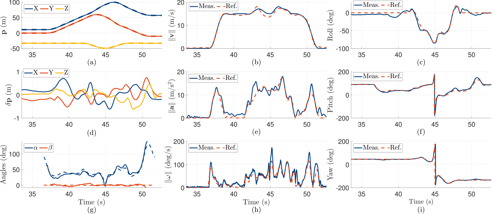
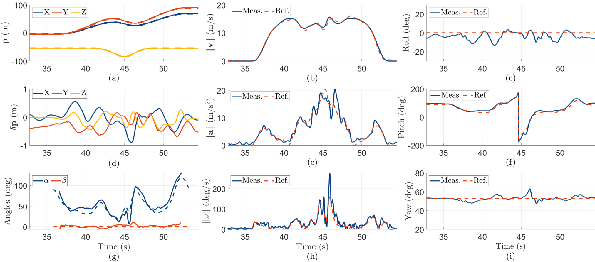


Fig. 28 details the flight data of the Wingover. The vehicle first transits from hovering to level flight with speed of , then performs the Wingover maneuver in 14- and finally ends with a backward transition to hovering. The vehicle climbs at the top and achieves the specified roll and yaw angle at . Note that the ZXY Euler angle incurs singularity in the visualization, but our global on-manifold MPC has no such singularity as shown in the FPV image in Fig. 23(b)D. Throughout the flight, the vehicle tracks all of the state trajectories closely: the position error is less than in all time and the sideslip angle is well stabilized around zero. This tracking accuracy is not trivial for outdoor UAV aerobatics with such large large span of angle of attack (up to ), acceleration (up to ), and angular velocity (up to ).
The flight results of the Loop is shown in Fig. 29. The vehicle transits to and successfully finishes a Loop with radius of around in . It is seen that the pitch angle rises to at , when the vehicle is totally upside-down at the top of the Loop as designed, which is also shown in Fig. 24(b)D. The vehicle also tracks all of the state trajectories closely in the coordinated flight condition (i.e., the sideslip angle is shown around zero). The position error also remains below in all directions, even though the maximum acceleration and angular velocity increase to and , respectively.
As shown in Fig. 30, the vehicle finishes a more aggressive aerobatic maneuver of Vertical Eight also in high tracking accuracy. From in level flight, the vehicle begins to pull up the pitch angle to and quickly lowers it to zero at , meanwhile the vehicle simultaneously gains altitude by following a “S”-shape trajectory (i.e., position A-B-C in Fig. 25(a)). After that, the vehicle flies another “S”-shape trajectory to decrease to the original altitude when the pitch angle continues to decrease to (i.e, nearly free falling as shown in Fig. 25(b)E) and quickly increases to to perform a level flight again. It is seen that the angle of attack ranges from to , the largest span among all the demonstrated aerobatics. Moreover, the acceleration and angular velocity respectively peak at and . Despite such large span of angle of attack and high acceleration and angular velocity, the overall position error still remains less than .
Similarly, the vehicle executes the Cuban Eight maneuver in high tracking performance despite the extremely high aggressiveness. The vehicle tracks the -shape with a width of , a height of , and a time duration of . The pitch angle increases from in level flight to at position C in Fig 26(a), then it decreases to at position E and recovers to at position F for level flight. The resulting span of angle of attack is about . The acceleration and angular velocity peaks at and , respectively. The maximum position error slightly rises to due to the large control actuation but the overall tracking performance for the other state trajectories are still as good as other aerobatic maneuvers.
Moreover, we demonstrate a Combo trajectory by connecting the above aerobatic maneuvers in sequence, as shown in Fig. 27. The vehicle performs the Combo maneuver which requires extremely large control actuation over the entire flight. In Fig. 32, it is seen that the thrust acceleration and angular velocity commands computed by the MPC frequently touch their limits, but the controller still manages to stabilize the vehicle under such control saturation.
The trajectory aggressiveness and tracking accuracy of the five aerobatic maneuvers in the Combo flight are statistically analyzed in Fig. 33. The maximum velocity, acceleration and angular velocity reach , and , respectively. Still, the proposed global controller shows a remarkable tracking performance that the average position tracking error is and largest position error is only . Readers are highly recommended to watch the accompanying videos for better visualization of the experiments.
8.5 Time consumption
The statistical time consumption of the trajectory planner and MPC in all of the above flight tests including flights, typical maneuvers, and aerobatic maneuvers is summarized in Fig. 34. For the trajectory generation in (48) which runs offline, the computation time is about 45- to generate one trajectory segment with a length of about 2.5-. The average and maximum time consumption to solve the MPC problem in (61) in total is and , respectively, showing a high computational efficiency ensuring online implementation at .
9 Conclusion
In this section, we discuss the limitation and extension of the proposed framework, and then draw the conclusion.
9.1 Limitation
Our proposed framework is a model-based approach. Higher tracking accuracy requires a more precise dynamic model, especially the aerodynamic model. However, identifying a high-fidelity aerodynamic model generally requires high-cost and time-consuming wind tunnel tests. The cost and time escalate for tail-sitter UAVs where the envelope of angle of attack is large. In this paper, we leveraged the wind tunnel test data in (Lyu et al. 2018a). For general tail-sitter UAVs, such aerodynamic model could be identified from onboard sensor data collected in real flights, which would be a promising future research to pursue.
Another limitation lies in the robustness and computation efficiency of the trajectory planner. In this paper, we adopted the MINCO trajectory optimization framework (Wang et al. 2022), which parameterizes the trajectory by a multi-stage polynomial and penalizes the constraints in the objective function as soft constraints. Softly penalizing the constraints in objective functions could reduce the optimization time by eliminating the hard constraints. However, due to the extremely nonlinear objective function, the solver could easily converge to local minimum violating the constraints. This phenomenon occasionally occurred in the planning of the outdoor aerobatic trajectories when the waypoints locations are poorly specified. Moreover, the optimization time is still quite long, 40-, preventing it from real-time implementation on current tail-sitter onboard computing devices.
9.2 Extension
Firstly, the proposed trajectory optimization could potentially be solved more efficiently by leveraging state-of-the-art nonlinear optimization techniques (e.g., Schulman et al. 2014; Gill et al. 2005), the availability of higher-performance onboard computing devices, and the parallelization of the optimization based on Graphic Processing Units (GPUs). With an efficient solution, the proposed trajectory generation could serve as a reliable back-end planner for on-line trajectory planning. Equipped with onboard sensors such as cameras and lidars, and the corresponding front-end corridor generation techniques (e.g., Liu et al. 2017; Gao et al. 2019), the tail-sitter could perform autonomous obstacle avoidance in cluttered environments.
Secondly, the tracking accuracy can be further improved by augmenting a low-level controller to the thrust acceleration . In the present implementation, we directly mapped the thrust acceleration command to the collective throttle of the four motors. However, the actual propeller thrust is also affected by various other factors, such as the propeller inflow (Brandt and Selig 2011; Gill and D’andrea 2017) and motor internal dynamics. These factors have caused significant errors between the actual and commanded thrust acceleration as shown in our experiment results. This issue could be mitigated by tracking the thrust acceleration command with a low-level controller based on accelerometer measurements.
Thirdly, other than the model predictive controller in the present implementation, the flatness function provides a possibility to design a more light-weight cascaded PID controller that runs on low-cost micro processors. The cascaded control architecture could be similar to that of a multicopter: an outer-loop position controller first computes the desired acceleration, then our differential flatness function maps the desired acceleration to the desired attitude and thrust, finally the attitude is tracked by an inner-loop attitude controller. Such a cascaded control structure is also used in existing works (Ritz and D’Andrea 2017; Cheng and Pei 2022), but based on an over-simplified aerodynamic model.
Finally, the proposed framework can be extended to other configurations of tail-sitter UAVs, such as the single-propeller configuration (Frank et al. 2007; Wang et al. 2017b; De Wagter et al. 2018) and the shoulder-mounted twin-engine configuration (Bapst et al. 2015; Ritz and D’Andrea 2017; Sun et al. 2018). All of he trajectory generation, flatness transform and global control for the high-level system can be directly applied to the other configurations, while the low-level controller could be re-designed according to the specific vehicle dynamic parameters and actuator performances.
9.3 Conclusion
In this paper, we proposed a trajectory generation and global tracking controller for aggressive agile tail-sitter flights. The foundation of the framework is the differential flatness property that is proved in coordinated flights. The singularity conditions occurred in the flatness function were fully investigated and resolved in the framework. Based on these theoretical results, we developed a trajectory optimization framework for trajectory generation and a model predictive controller for trajectory tracking. The entire approach is tested on a quadrotor tail-sitter prototype in extensive real-world flights. Notably, we demonstrated agile flights in indoor environments and aerobatic maneuvers in windy outdoor environments, which were rarely shown in any prior literature works. Extensive flight tests on typical maneuvers of transition, level flight and loiter, have also shown a superior tracking accuracy compared to existing methods.
Acknowledgment
This work was supported in part by Hong Kong RGC ECS under grant 27202219 and in part by DJI donation. The authors appreciate Dr. Wei Xu and Dr. Haowei Gu for the help on the initial set up of the prototype, and Huirong Cheng for discussion. The author especially thank Dr. Ximin Lyu of Sun Yat-sen University for providing the space and equipment for conducting the indoor experiments.
References
- Bapst et al. (2015) Bapst R, Ritz R, Meier L and Pollefeys M (2015) Design and implementation of an unmanned tail-sitter. In: 2015 IEEE/RSJ international conference on intelligent robots and systems (IROS). IEEE, pp. 1885–1890.
- Barth et al. (2020) Barth JM, Condomines JP, Bronz M, Moschetta JM, Join C and Fliess M (2020) Model-free control algorithms for micro air vehicles with transitioning flight capabilities. International Journal of Micro Air Vehicles 12: 1756829320914264.
- Borrelli et al. (2017) Borrelli F, Bemporad A and Morari M (2017) Predictive control for linear and hybrid systems. Cambridge University Press.
- Brandt and Selig (2011) Brandt J and Selig M (2011) Propeller performance data at low reynolds numbers. In: 49th AIAA Aerospace Sciences Meeting including the New Horizons Forum and Aerospace Exposition. p. 1255.
- Bry et al. (2015) Bry A, Richter C, Bachrach A and Roy N (2015) Aggressive flight of fixed-wing and quadrotor aircraft in dense indoor environments. The International Journal of Robotics Research 34(7): 969–1002.
- Bullo and Murray (1995) Bullo F and Murray RM (1995) Proportional derivative (pd) control on the euclidean group .
- Carlson (2014) Carlson S (2014) A hybrid tricopter/flying-wing vtol uav. In: 52nd Aerospace Sciences Meeting. p. 0016.
- Çetinsoy et al. (2011) Çetinsoy E, Sirimoğlu E, Öner KT, Hancer C, Ünel M, Akşit MF, Kandemir I and Gülez K (2011) Design and development of a tilt-wing uav. Turkish Journal of Electrical Engineering and Computer Sciences 19(5): 733–741.
- Cheng and Pei (2022) Cheng ZH and Pei HL (2022) Transition analysis and practical flight control for ducted fan fixed-wing aerial robot: Level path flight mode transition. IEEE Robotics and Automation Letters 7(2): 3106–3113.
- Chitsaz and LaValle (2007) Chitsaz H and LaValle SM (2007) Time-optimal paths for a dubins airplane. In: 2007 46th IEEE conference on decision and control. IEEE, pp. 2379–2384.
- Clancy (1975) Clancy LJ (1975) Aerodynamics. John Wiley & Sons.
- De Wagter et al. (2018) De Wagter C, Ruijsink R, Smeur EJ, van Hecke KG, van Tienen F, van der Horst E and Remes BD (2018) Design, control, and visual navigation of the delftacopter vtol tail-sitter uav. Journal of Field Robotics 35(6): 937–960.
- Ding et al. (2019) Ding W, Gao W, Wang K and Shen S (2019) An efficient b-spline-based kinodynamic replanning framework for quadrotors. IEEE Transactions on Robotics 35(6): 1287–1306.
- Etkin and Reid (1959) Etkin B and Reid LD (1959) Dynamics of flight, volume 2. Wiley New York.
- Faessler et al. (2017) Faessler M, Franchi A and Scaramuzza D (2017) Differential flatness of quadrotor dynamics subject to rotor drag for accurate tracking of high-speed trajectories. IEEE Robotics and Automation Letters 3(2): 620–626.
- Falanga et al. (2018) Falanga D, Foehn P, Lu P and Scaramuzza D (2018) Pampc: Perception-aware model predictive control for quadrotors. In: 2018 IEEE/RSJ International Conference on Intelligent Robots and Systems (IROS). IEEE, pp. 1–8.
- Falanga et al. (2017) Falanga D, Mueggler E, Faessler M and Scaramuzza D (2017) Aggressive quadrotor flight through narrow gaps with onboard sensing and computing using active vision. In: 2017 IEEE international conference on robotics and automation (ICRA). IEEE, pp. 5774–5781.
- Fliess et al. (1995) Fliess M, Lévine J, Martin P and Rouchon P (1995) Flatness and defect of non-linear systems: introductory theory and examples. International journal of control 61(6): 1327–1361.
- Foehn et al. (2021) Foehn P, Romero A and Scaramuzza D (2021) Time-optimal planning for quadrotor waypoint flight. Science Robotics 6(56): eabh1221.
- Frank et al. (2007) Frank A, McGrew J, Valenti M, Levine D and How J (2007) Hover, transition, and level flight control design for a single-propeller indoor airplane. In: AIAA Guidance, Navigation and Control Conference and Exhibit. p. 6318.
- Gao et al. (2019) Gao F, Wu W, Gao W and Shen S (2019) Flying on point clouds: Online trajectory generation and autonomous navigation for quadrotors in cluttered environments. Journal of Field Robotics 36(4): 710–733.
- Gertz and Wright (2003) Gertz EM and Wright SJ (2003) Object-oriented software for quadratic programming. ACM Transactions on Mathematical Software (TOMS) 29(1): 58–81.
- Gill et al. (2005) Gill PE, Murray W and Saunders MA (2005) Snopt: An sqp algorithm for large-scale constrained optimization. SIAM review 47(1): 99–131.
- Gill and D’andrea (2017) Gill R and D’andrea R (2017) Propeller thrust and drag in forward flight. In: 2017 IEEE Conference on Control Technology and Applications (CCTA). IEEE, pp. 73–79.
- Gu et al. (2018) Gu H, Cai X, Zhou J, Li Z, Shen S and Zhang F (2018) A coordinate descent method for multidisciplinary design optimization of electric-powered winged uavs. In: 2018 International Conference on Unmanned Aircraft Systems (ICUAS). IEEE, pp. 1189–1198.
- Gu et al. (2017) Gu H, Lyu X, Li Z, Shen S and Zhang F (2017) Development and experimental verification of a hybrid vertical take-off and landing (vtol) unmanned aerial vehicle (uav). In: 2017 International Conference on Unmanned Aircraft Systems (ICUAS). IEEE, pp. 160–169.
- Hang et al. (2019) Hang K, Lyu X, Song H, Stork JA, Dollar AM, Kragic D and Zhang F (2019) Perching and resting—a paradigm for uav maneuvering with modularized landing gears. Science Robotics 4(28): eaau6637.
- Hauser et al. (1992) Hauser J, Sastry S and Meyer G (1992) Nonlinear control design for slightly non-minimum phase systems: Application to v/stol aircraft. Automatica 28(4): 665–679.
- Hertzberg et al. (2013) Hertzberg C, Wagner R, Frese U and Schröder L (2013) Integrating generic sensor fusion algorithms with sound state representations through encapsulation of manifolds. Information Fusion 14(1): 57–77.
- Johansen et al. (2015) Johansen TA, Cristofaro A, Sørensen K, Hansen JM and Fossen TI (2015) On estimation of wind velocity, angle-of-attack and sideslip angle of small uavs using standard sensors. In: 2015 International Conference on Unmanned Aircraft Systems (ICUAS). IEEE, pp. 510–519.
- Jung and Shim (2012) Jung Y and Shim DH (2012) Development and application of controller for transition flight of tail-sitter uav. Journal of Intelligent & Robotic Systems 65(1): 137–152.
- Kamel et al. (2017) Kamel M, Burri M and Siegwart R (2017) Linear vs nonlinear mpc for trajectory tracking applied to rotary wing micro aerial vehicles. IFAC-PapersOnLine 50(1): 3463–3469.
- Kaufmann et al. (2020) Kaufmann E, Loquercio A, Ranftl R, Müller M, Koltun V and Scaramuzza D (2020) Deep drone acrobatics. RSS: Robotics, Science, and Systems .
- Kita et al. (2010) Kita K, Konno A and Uchiyama M (2010) Transition between level flight and hovering of a tail-sitter vertical takeoff and landing aerial robot. Advanced Robotics 24(5-6): 763–781.
- Lambregts (1983) Lambregts A (1983) Vertical flight path and speed control autopilot design using total energy principles. In: Guidance and Control Conference. p. 2239.
- Li et al. (2020a) Li B, Sun J, Zhou W, Wen CY, Low KH and Chen CK (2020a) Transition optimization for a vtol tail-sitter uav. IEEE/ASME transactions on mechatronics 25(5): 2534–2545.
- Li et al. (2018) Li B, Zhou W, Sun J, Wen CY and Chen CK (2018) Development of model predictive controller for a tail-sitter vtol uav in hover flight. Sensors 18(9): 2859.
- Li et al. (2020b) Li Y, Qin Y, Xu W and Zhang F (2020b) Modeling, identification, and control of non-minimum phase dynamics of bi-copter uavs. In: 2020 IEEE/ASME International Conference on Advanced Intelligent Mechatronics (AIM). IEEE, pp. 1249–1255.
- Liu et al. (2017) Liu S, Watterson M, Mohta K, Sun K, Bhattacharya S, Taylor CJ and Kumar V (2017) Planning dynamically feasible trajectories for quadrotors using safe flight corridors in 3-d complex environments. IEEE Robotics and Automation Letters 2(3): 1688–1695.
- Lu et al. (2022) Lu G, Xu W and Zhang F (2022) On-manifold model predictive control for trajectory tracking on robotic systems. IEEE Transactions on Industrial Electronics .
- Lustosa (2017) Lustosa LR (2017) The Phi-theory approach to flight control design of hybrid vehicles. PhD Thesis, PhD thesis, ISAE-SUPAERO.
- Lustosa et al. (2019) Lustosa LR, Defaÿ F and Moschetta JM (2019) Global singularity-free aerodynamic model for algorithmic flight control of tail sitters. Journal of Guidance, Control, and Dynamics 42(2): 303–316.
- Lyu et al. (2017a) Lyu X, Gu H, Wang Y, Li Z, Shen S and Zhang F (2017a) Design and implementation of a quadrotor tail-sitter vtol uav. In: 2017 IEEE international conference on robotics and automation (ICRA). IEEE, pp. 3924–3930.
- Lyu et al. (2017b) Lyu X, Gu H, Zhou J, Li Z, Shen S and Zhang F (2017b) A hierarchical control approach for a quadrotor tail-sitter vtol uav and experimental verification. In: 2017 IEEE/RSJ International Conference on Intelligent Robots and Systems (IROS). IEEE, pp. 5135–5141.
- Lyu et al. (2018a) Lyu X, Gu H, Zhou J, Li Z, Shen S and Zhang F (2018a) Simulation and flight experiments of a quadrotor tail-sitter vertical take-off and landing unmanned aerial vehicle with wide flight envelope. International Journal of Micro Air Vehicles 10(4): 303–317.
- Lyu et al. (2018b) Lyu X, Zhou J, Gu H, Li Z, Shen S and Zhang F (2018b) Disturbance observer based hovering control of quadrotor tail-sitter vtol uavs using synthesis. IEEE Robotics and Automation Letters 3(4): 2910–2917.
- Marion (2021) Marion P (2021) Flipping the script with atlas. URL https://www.bostondynamics.com/resources/blog/flipping-script-atlas. Accessed on 08 23, 2021.
- Martin et al. (1996) Martin P, Devasia S and Paden B (1996) A different look at output tracking: Control of a vtol aircraft. Automatica 32(1): 101–107.
- Matsumoto et al. (2010) Matsumoto T, Kita K, Suzuki R, Oosedo A, Go K, Hoshino Y, Konno A and Uchiyama M (2010) A hovering control strategy for a tail-sitter vtol uav that increases stability against large disturbance. In: 2010 IEEE international conference on robotics and automation. IEEE, pp. 54–59.
- Mayne et al. (2000) Mayne DQ, Rawlings JB, Rao CV and Scokaert PO (2000) Constrained model predictive control: Stability and optimality. Automatica 36(6): 789–814.
- McIntosh and Mishra (2022) McIntosh K and Mishra S (2022) Transition trajectory planning and control for quadrotor biplanes in obstacle cluttered environments .
- McKenna (2007) McKenna J (2007) One step beyond, rotor wing.
- Meier et al. (2015) Meier L, Honegger D and Pollefeys M (2015) Px4: A node-based multithreaded open source robotics framework for deeply embedded platforms. In: 2015 IEEE international conference on robotics and automation (ICRA). IEEE, pp. 6235–6240.
- Mellinger and Kumar (2011) Mellinger D and Kumar V (2011) Minimum snap trajectory generation and control for quadrotors. In: 2011 IEEE international conference on robotics and automation. IEEE, pp. 2520–2525.
- Mellinger et al. (2012) Mellinger D, Michael N and Kumar V (2012) Trajectory generation and control for precise aggressive maneuvers with quadrotors. The International Journal of Robotics Research 31(5): 664–674.
- Mueller et al. (2015) Mueller MW, Hehn M and D’Andrea R (2015) A computationally efficient motion primitive for quadrocopter trajectory generation. IEEE transactions on robotics 31(6): 1294–1310.
- Murray et al. (1995) Murray RM, Rathinam M and Sluis W (1995) Differential flatness of mechanical control systems: A catalog of prototype systems. In: ASME international mechanical engineering congress and exposition. Citeseer.
- Naldi and Marconi (2011) Naldi R and Marconi L (2011) Optimal transition maneuvers for a class of v/stol aircraft. Automatica 47(5): 870–879.
- Nguyen et al. (2021) Nguyen H, Kamel M, Alexis K and Siegwart R (2021) Model predictive control for micro aerial vehicles: A survey. In: 2021 European Control Conference (ECC). IEEE, pp. 1556–1563.
- Noormohammadi-Asl et al. (2020) Noormohammadi-Asl A, Esrafilian O, Arzati MA and Taghirad HD (2020) System identification and -based control of quadrotor attitude. Mechanical Systems and Signal Processing 135: 106358.
- Oosedo et al. (2013) Oosedo A, Abiko S, Konno A, Koizumi T, Furui T and Uchiyama M (2013) Development of a quad rotor tail-sitter vtol uav without control surfaces and experimental verification. In: 2013 IEEE international conference on robotics and automation. IEEE, pp. 317–322.
- Oosedo et al. (2017) Oosedo A, Abiko S, Konno A and Uchiyama M (2017) Optimal transition from hovering to level-flight of a quadrotor tail-sitter uav. Autonomous Robots 41(5): 1143–1159.
- Ozdemir et al. (2014) Ozdemir U, Aktas YO, Vuruskan A, Dereli Y, Tarhan AF, Demirbag K, Erdem A, Kalaycioglu GD, Ozkol I and Inalhan G (2014) Design of a commercial hybrid vtol uav system. Journal of Intelligent & Robotic Systems 74(1): 371–393.
- Park (2014) Park R (2014) Arcturus uav upgrades the jump15 vtol uav. Airlines & Aviation, Aerospace & Defense .
- Park et al. (2004) Park S, Deyst J and How J (2004) A new nonlinear guidance logic for trajectory tracking. In: AIAA guidance, navigation, and control conference and exhibit. p. 4900.
- Pucci (2012) Pucci D (2012) Flight dynamics and control in relation to stall. In: 2012 American Control Conference (ACC). IEEE, pp. 118–124.
- Pucci et al. (2013) Pucci D, Hamel T, Morin P and Samson C (2013) Nonlinear control of aerial vehicles subjected to aerodynamic forces. In: 52nd IEEE Conference on Decision and Control. IEEE, pp. 4839–4846.
- Ren et al. (2023) Ren Y, Liang S, Zhu F, Lu G and Zhang F (2023) Online whole-body motion planning for quadrotor using multi-resolution search. In: 2023 IEEE International Conference on Robotics and Automation (ICRA). pp. 1594–1600. 10.1109/ICRA48891.2023.10160767.
- Ritz and D’Andrea (2017) Ritz R and D’Andrea R (2017) A global controller for flying wing tailsitter vehicles. In: 2017 IEEE international conference on robotics and automation (ICRA). IEEE, pp. 2731–2738.
- Romero et al. (2022) Romero A, Penicka R and Scaramuzza D (2022) Time-optimal online replanning for agile quadrotor flight. IEEE Robotics and Automation Letters 7(3): 7730–7737.
- Schulman et al. (2014) Schulman J, Duan Y, Ho J, Lee A, Awwal I, Bradlow H, Pan J, Patil S, Goldberg K and Abbeel P (2014) Motion planning with sequential convex optimization and convex collision checking. The International Journal of Robotics Research 33(9): 1251–1270.
- Shen et al. (2011) Shen S, Michael N and Kumar V (2011) Autonomous multi-floor indoor navigation with a computationally constrained mav. In: 2011 IEEE International Conference on Robotics and Automation. IEEE, pp. 20–25.
- Smeur et al. (2020) Smeur EJ, Bronz M and de Croon GC (2020) Incremental control and guidance of hybrid aircraft applied to a tailsitter unmanned air vehicle. Journal of Guidance, Control, and Dynamics 43(2): 274–287.
- Stevens et al. (2015) Stevens BL, Lewis FL and Johnson EN (2015) Aircraft control and simulation: dynamics, controls design, and autonomous systems. John Wiley & Sons.
- Sun et al. (2018) Sun J, Li B, Wen CY and Chen CK (2018) Design and implementation of a real-time hardware-in-the-loop testing platform for a dual-rotor tail-sitter unmanned aerial vehicle. Mechatronics 56: 1–15.
- Sun et al. (2022) Sun S, Romero A, Foehn P, Kaufmann E and Scaramuzza D (2022) A comparative study of nonlinear mpc and differential-flatness-based control for quadrotor agile flight. IEEE Transactions on Robotics : 1–1710.1109/TRO.2022.3177279.
- Tal and Karaman (2022) Tal E and Karaman S (2022) Global incremental flight control for agile maneuvering of a tailsitter flying wing. Journal of Guidance, Control, and Dynamics 45(12): 2332–2349.
- Tal et al. (2022) Tal E, Ryou G and Karaman S (2022) Aerobatic trajectory generation for a vtol fixed-wing aircraft using differential flatness. arXiv preprint arXiv:2207.03524 .
- Tal and Karaman (2021) Tal EA and Karaman S (2021) Global trajectory-tracking control for a tailsitter flying wing in agile uncoordinated flight. In: AIAA AVIATION 2021 FORUM. p. 3214.
- Van Nieuwstadt and Murray (1998) Van Nieuwstadt MJ and Murray RM (1998) Rapid hover-to-forward-flight transitions for a thrust-vectored aircraft. Journal of Guidance, Control, and Dynamics 21(1): 93–100.
- Verling et al. (2016) Verling S, Weibel B, Boosfeld M, Alexis K, Burri M and Siegwart R (2016) Full attitude control of a vtol tailsitter uav. In: 2016 IEEE international conference on robotics and automation (ICRA). IEEE, pp. 3006–3012.
- Vourtsis et al. (2023) Vourtsis C, Rochel VC, Müller NS, Stewart W and Floreano D (2023) Wind defiant morphing drones. Advanced Intelligent Systems 5(3): 2200297.
- Wang et al. (2017a) Wang K, Ke Y, Lai S, Gong K, Tan Y and Chen BM (2017a) Model-based optimal auto-transition and control synthesis for tail-sitter uav kh-lion. In: 2017 13th IEEE International Conference on Control & Automation (ICCA). IEEE, pp. 541–547.
- Wang et al. (2017b) Wang W, Zhu J and Kuang M (2017b) Design, modelling and hovering control of a tail-sitter with single thrust-vectored propeller. In: 2017 IEEE/RSJ International Conference on Intelligent Robots and Systems (IROS). IEEE, pp. 5971–5976.
- Wang et al. (2022) Wang Z, Zhou X, Xu C and Gao F (2022) Geometrically constrained trajectory optimization for multicopters. IEEE Transactions on Robotics .
- Xu et al. (2019a) Xu W, Gu H, Qing Y, Lin J and Zhang F (2019a) Full attitude control of an efficient quadrotor tail-sitter vtol uav with flexible modes. In: 2019 International Conference on Unmanned Aircraft Systems (ICUAS). IEEE, pp. 542–550.
- Xu et al. (2019b) Xu W, Gu H and Zhang F (2019b) Acceleration based iterative learning control for pugachev’s cobra maneuver with quadrotor tailsitter vtol uavs. work 7: 12.
- Zhang et al. (2020) Zhang J, Hu C, Chadha RG and Singh S (2020) Falco: Fast likelihood-based collision avoidance with extension to human-guided navigation. Journal of Field Robotics 37(8): 1300–1313.
- Zhou et al. (2019) Zhou B, Gao F, Wang L, Liu C and Shen S (2019) Robust and efficient quadrotor trajectory generation for fast autonomous flight. IEEE Robotics and Automation Letters 4(4): 3529–3536.
- Zhou et al. (2018) Zhou J, Lyu X, Cai X, Li Z, Shen S and Zhang F (2018) Frequency domain model identification and loop-shaping controller design for quadrotor tail-sitter vtol uavs. In: 2018 International Conference on Unmanned Aircraft Systems (ICUAS). IEEE, pp. 1142–1149.
- Zhou et al. (2017) Zhou J, Lyu X, Li Z, Shen S and Zhang F (2017) A unified control method for quadrotor tail-sitter uavs in all flight modes: Hover, transition, and level flight. In: 2017 IEEE/RSJ International Conference on Intelligent Robots and Systems (IROS). IEEE, pp. 4835–4841.
Appendix A Proof of theorem 1
Given the vehicle dynamics in (1), the rank of system dynamics derivative w.r.t input can be given by eliminating unrelated items:
| (65) | ||||
where the following elements can be computed directly from the system dynamics in (1):
| (66) |
and has coupling effect due to the coordinated flight condition that the vehicle has no lateral airspeed:
| (67) |
which leads to the derivative on the both sides:
| (68a) | ||||
| (68b) | ||||
| (68c) | ||||
It is seen that the body angular velocity elements and are coupled. Without loss of generality, we consider as a function of . Then we have
| (69) |
Appendix B Proof of theorem 2
Reminding the aerodynamic force in (6) and the coordinated flight condition that there is no lateral airspeed in (27) (i.e., ) , we have
| (72) |
where
| (73a) | ||||
| (73b) | ||||
| (73c) | ||||
and the aerodynamic coefficient gradients and of an axially symmetric airframe satisfies (11). Substituting (73) into (72), we have
| (74) |
Appendix C Calculation of matrices and
Appendix D Proof of Theorem 3 (determinant of )
We first denote
| (78) |
With (20), we have
| (79) |
Now we calculate the determinant of . With (30c) and (30d), can be factorized as
| (83) |
which implies . Performing elementary row and column operations on produces
| (84) |
By substituting (82) into (84), the determinant of hence can be calculated as follows:
| (85) |
It is noted that the derivative of (22) w.r.t. is given as
| (86) |
Therefore, the determinant of is finally arrived at
| (87) |
Appendix E Singularity
E.1 Proof of Theorem 4: determinant of
E.2 Calculation of and
As and break into block matrices, their derivatives and can be presented as like (75), where each block is calculated as follows:
| (91a) | ||||
| (91b) | ||||
| (91c) | ||||
| (91d) | ||||
Appendix F Singularity
F.1 Proof of Theorem 5: determinant of
Because is perpendicular to , so it still holds the lateral airspeed condition . We can leverage the results in (81), (82) and (86) in Appendix D to factorize as follows:
| (92) |
which implies . Performing elementary row and column operations on produces
| (93) |
where is from (82c) by setting , and is from (86). Finally, the determinant of is
| (94) |
F.2 Calculation of and
Appendix G Gradients of the flatness functions
G.1 When in coordinated flight
The flatness functions are presented in Section 4.2, and the corresponding gradients are given as follows:
| (95a) | ||||
| (95b) | ||||
where
| (96a) | ||||
| (96b) | ||||
| (96c) | ||||
| (96d) | ||||
| (96e) | ||||
| (96f) | ||||
| (96g) | ||||
| (96h) | ||||
| (96i) | ||||
| (96j) | ||||
| (96k) | ||||
| (96l) | ||||
| (96m) | ||||
| (96n) | ||||
| (96o) | ||||
| (96p) | ||||
| (96q) | ||||
| (96r) | ||||
| (96s) | ||||
| (96t) | ||||
| (96u) | ||||
G.2 When in singularity condition
G.3 When in singularity condition
Appendix H Proof of Theorem 6 (the error-state dynamics)
The dynamics of (56b) and (56c) simply take the time derivative to (54b) and (54c), respectively. Denoting , the exponential map holds , where , the inverse of that maps a skew-symmetric matrix to a vector, and denotes the Jacobian of the exponential coordinates of (Bullo and Murray 1995):
| (98) |
By substituting (54b) into the above rules, we have
| (99) |
which is the error attitude dynamics in (56d).
Appendix I Proof of Lemma 1 (the linearized error-state dynamics)
The position error dynamics in (56b) is linear, and the velocity error dynamics in (56c) can be linearized along the reference trajectory. Specifically, since , (54) implies:
| (100) | ||||
where
| (101a) | ||||
| (101b) | ||||
and the partial derivative in (101a) is given in (74):
| (102) |