Mean-field neural networks-based algorithms for McKean-Vlasov control problems Thanks: This work is supported by FiME, Laboratoire de Finance des Marchés de l’Energie, and the “Finance and Sustainable Development” EDF - CACIB Chair.

Solution to the MKV control problem (1.1) can be characterized by dynamic programming (DP) or maximum principle methods (see [6] for a detailed treatment of this topic). We recall the main results that will be used for designing our algorithms. In the DP approach, one considers the dynamic version of problem (1.1) by defining the decoupled value function $V$ defined on $[0,T]\times\mathbb{R}^{d}\times{\cal P}_{2}(\mathbb{R}^{d})$, which satisfies the backward recursion:

for any $t$ $\in$ $[0,T)$, $h$ $\in$ $(0,T-t]$, and starting from the terminal condition $V(T,x,\mu)$ $=$ $g(x,\mu)$, for $(x,\mu)$ $\in$ $[0,T]\times{\cal P}_{2}(\mathbb{R}^{d})$, so that $v(\mu_{0})$ $=$ $\mathbb{E}[V(0,X_{0},\mu_{0})]$. By sending $h$ to zero, we derive the master Bellman equation for the value function (see section 6.5.2 in [6])

for $(t,x,\mu)$ $\in$ $[0,T)\times\mathbb{R}^{d}\times{\cal P}_{2}(\mathbb{R}^{d})$. Here $\cdot$ is the inner product in Euclidian spaces, ^⊺ is the transpose operator for a matrix, $x^{\prime}$ $\in$ $\mathbb{R}^{d}$ $\mapsto$ $\partial_{\mu}V(t,x,\mu)(x^{\prime})$ $\in$ $\mathbb{R}^{d}$ is the Lions derivative on ${\cal P}_{2}(\mathbb{R}^{d})$ (see [6]), the notation $\mathbb{E}_{\xi\sim\mu}[.]$ means that the expectation is taken w.r.t. the random variable $\xi$ distributed according to the law $\mu$,

and it is assumed that for any $(x,\mu,p,M)$ $\in$ $\mathbb{R}^{d}\times{\cal P}_{2}(\mathbb{R}^{d})\times\mathbb{R}^{d}\times\mathbb{R}^{d\times d}$, there exists a minimizer

which is Lipschitz in all its variables, so that we get an optimal feedback control given by

In the case where the diffusion coefficient $\sigma(x,\mu)$ does not depend on the control variable $a$, and so $\hat{\mathrm{a}}(x,\mu,p)$ does not depend on the variable $M$, we have a probabilistic characterization of the solution in terms of forward-backward SDE of MKV type: by setting

it follows from Itô’s formula and Master Bellman equation that $(X,Y,Z)$ satisfies the forward-backward SDE

where the pair $(P_{t},M_{t})_{t}$ $=$ $({\cal U}(t,X_{t},\mathbb{P}_{X_{t}}),\partial_{x}{\cal U}(t,X_{t},\mathbb{P}_{X_{t}})\sigma(X_{t},\mathbb{P}_{X_{t}}))_{t}$ of adjoint processes, valued in $\mathbb{R}^{d}\times\mathbb{R}^{d\times d}$, satisfies from the Pontryagin maximum principle the backward SDE:

where $(\tilde{X},\tilde{P},\tilde{M})$ are independent copies of $(X,P,M)$ on $(\tilde{\Omega},\tilde{\cal F},\tilde{\mathbb{P}})$. Under the assumption that $(x,\mu)$ $\in$ $\mathbb{R}^{d}\times{\cal P}_{2}(\mathbb{R}^{d})$ $\mapsto$ $g(x,\mu)$ is convex, $(x,\mu,a)$ $\in$ $\mathbb{R}^{d}\times{\cal P}_{2}(\mathbb{R}^{d})\times A$ (with $A$ convex set) $\mapsto$ $H(x,\mu,p,M,a)$ is convex for any $(p,M)$, together with additional regularity conditions on the coefficients $b,\sigma,f,g$, it is known from [5] that the solution to the adjoint BSDE (2.14) yields an optimal control given by

We are then led to consider the generic form of MKV forward-backward $(X,{\cal Y},{\cal Z})$:

The solution to MKV control problem, i.e., the value function and optimal feedback control, are mappings of the state process and its probability distribution. In order to approximate such mappings, we shall rely on mean-field neural networks introduced in our companion paper [25]. Those are mappings

in one of the following forms:

• (i)

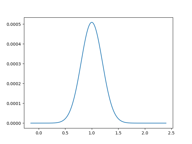
  Bin density: ${\cal N}(\mu)(x)$ $=$ $\Phi(x,{\boldsymbol{p}}^{\mu})$, for $x$ $\in$ $\mathbb{R}^{d}$, $\mu$ $\in$ ${\cal D}_{2}(\mathbb{R}^{d})$ the subset of probability measures $\mu$ in ${\cal P}_{2}(\mathbb{R}^{d})$ which admit density functions $\mathrm{p}^{\mu}$ with respect to the Lebesgue measure $\lambda_{d}$ on $\mathbb{R}^{d}$. Here, $\Phi$ is a standard feedforward neural network from $\mathbb{R}^{d}\times\mathbb{R}^{K}$ into $\mathbb{R}^{p}$, and ${\boldsymbol{p}}^{\mu}$ $=$ $(p_{k}^{\mu})_{k\in\llbracket 1,K\rrbracket}$ is the bin weight of the discrete density approximation of $\mathrm{p}^{\mu}$ on a fixed bounded rectangular domain ${\cal K}$ of $\mathbb{R}^{d}$ divided into $K$ bins: $\cup_{k=1}^{K}{\rm Bin}(k)$ $=$ ${\cal K}$, of center $x_{k}$, with same area size $h$ $=$ $\lambda_{d}({\cal K})/K$, hence given by (see Figure 1 in the case of one dimensional Gaussian distribution for $\mu$):

  $\displaystyle p^{\mu}_{k}$

  $\displaystyle=$

  $\displaystyle\frac{\mathrm{p}^{\mu}(x_{k})}{\sum_{k=1}^{K}\mathrm{p}^{\mu}(x_{k})h},\quad k=1,\ldots,K.$

• (ii)

  Cylindrical: ${\cal N}(\mu)(\cdot)$ $=$ $\Psi(\cdot,<\varphi,\mu>)$, where $\Psi$ is a feedforward network function (outer neural network) from $\mathbb{R}^{d}\times\mathbb{R}^{q}$ into $\mathbb{R}^{p}$, and $\varphi$ is another feedforward network function (inner neural network) from $\mathbb{R}^{d}$ into $\mathbb{R}^{q}$ (called latent space). Here we denote $<\varphi,\mu>$ $:=$ $\int\varphi(x)\mu(\mathrm{d}x)$.

The relevance of mean-field neural networks is theoretically justified in [25] by universal approximation theorems, and it has been also shown how they can be trained accurately from samples of probability measures $\mu$ $=$ ${\cal L}_{D}({\boldsymbol{p}})$ with discrete density of bin weight ${\boldsymbol{p}}$ $=$ $(p^{k})_{k\in\llbracket 1,K\rrbracket}$ drawn randomly on ${\cal D}_{K}$ $=$ $\{{\boldsymbol{p}}=(p_{k})_{k\in\llbracket 1,K\rrbracket}\in\mathbb{R}_{+}^{K}:\sum_{k=1}^{K}p_{k}h=1\}$, and simulations of random variables $X$ $\sim$ $\mu$ by inverse transform. Notice that for $\mu$ $=$ ${\cal L}_{D}({\boldsymbol{p}})$, we have ${\boldsymbol{p}}^{\mu}$ $=$ ${\boldsymbol{p}}$, and so the bin density network at such $\mu$ is equal to ${\cal N}(\mu)(.)$ $=$ $\Phi(.,{\boldsymbol{p}})$. On the other hand, for any cylindrical function $F$ of the measure of the form $F(\mu)$ $=$ $\Psi(<\varphi,\mu>)$, we can compute it approximately from samples $X^{(n)}$, $n$ $=$ $1,\ldots,N$, of $\mu$ by: $F(\mu)$ $\simeq$ $\Psi\big(\frac{1}{N}\sum_{n=1}^{N}\varphi(X^{(n)})\big)$. This is the case in particular for cylindrical neural network.

As described in [25], exploring the space of probability measures is crucial for both neural networks. In both cases, we employ the bins method to generate samples of probability measures for training mean-field neural networks. The algorithm used to generate these measures is outlined in [25] and is currently limited to dimension one. Consequently, all numerical tests conducted in the article are confined to dimension one. However, it is possible to handle cases in dimension two by employing a different algorithm proposed in [29]. In all subsequent algorithms, the proper selection of the domain ${\cal K}$ is crucial, particularly for the bins method. When the support of the distribution is unknown, an iterative procedure becomes necessary. Two algorithms can be implemented as follows:

• 1.

  First algorithm: (i) Initially, make an initial guess of the support. (ii) Once the resolution is obtained, verify that the generated distribution’s support is primarily contained within ${\cal K}$, sufficiently far from its boundary. (iii) If the support is not mainly within ${\cal K}$, adapt the size and center of ${\cal K}$ accordingly.

• 2.

  Second algorithm: (i) Use a very large ${\cal K}$ during the first iteration to locate the domain of importance, employing a coarse resolution. (ii) In the subsequent calculation, reduce the size of ${\cal K}$ to achieve an accurate resolution.

In the spirit of the method introduced in [17], [18], which does not actually rely on dynamic programming, we replace feedback controls by time-dependent mean-field neural networks ${\cal N}(t,\mu)(x)$ valued in $A$ $\subset$ $\mathbb{R}^{m}$, with input $t$ $\in$ $[0,T]$, $\mu$ $\in$ ${\cal P}_{2}(\mathbb{R}^{d})$, and $x$ $\in$ $\mathbb{R}^{d}$, and minimize over the parameters $\theta$ of this mean-field neural network ${\cal N}$ $=$ ${\cal N}_{\theta}$ the global cost function

with

In practice, for $i$ $=$ $1,\ldots,N_{T}$, $\mu_{i}$ has to be estimated/approximated from samples of $X_{i}$, and this is done as follows. We use a training batch of $M$ probability measures $\mu_{0}^{(m)}$ $=$ ${\cal L}_{D}({\boldsymbol{p}}^{(m)})$ in ${\cal D}_{2}(\mathbb{R}^{d})$ from samples ${\boldsymbol{p}}^{(m)}$ $=$ $(p_{k}^{(m)})_{k\in\llbracket 1,K\rrbracket}$, $m$ $=$ $1,\ldots,M$, in ${\cal D}_{K}$. Then, for each $m$, we sample $X_{0}^{(m),(n)}$, $n$ $=$ $1,\ldots,N$, from $\mu_{0}^{(m)}$, and for $i$ $=$ $0,\ldots,N_{T}-1$, $X_{i+1}^{(m),(n)}$, $n$ $=$ $1,\ldots,N$ are sampled as

with $\hat{\mu}_{i}^{(m)}$ $=$ ${\cal L}_{D}(\hat{\boldsymbol{p}}_{i}^{(m)})$, $\hat{\boldsymbol{p}}_{0}^{(m)}$ $=$ ${\boldsymbol{p}}^{(m)}$, and $\hat{\boldsymbol{p}}_{i}^{(m)}$ $=$ $(\hat{p}_{i,k}^{(m)})_{k\in\llbracket 1,K\rrbracket}$ are the estimated density weights in ${\cal D}_{K}$ of $X_{i}^{(m),(n)}$, $i$ $=$ $1,\ldots,N_{T}$ (truncated on ${\cal K}$), namely:

where ${\rm Proj}_{{\cal K}}(.)$ is the projection on ${\cal K}$. The cost function is then approximated by

The pseudo-code using a gradient descent method is described in Algorithm 1.

The global algorithms that directly minimize the objective function have demonstrated effectiveness in practice, even without having a theoretical convergence proof. The output of this global algorithm is an approximation of the optimal feedback control at initial time $t_{0}$ $=$ $0$ by a mean-field neural network ${\cal N}_{\theta^{*}}(t_{0},.)$, and yields an approximation of the optimal control at other times $t_{i}$, $i$ $=$ $1,\ldots,N_{T}-1$, by mean-field neural networks ${\cal N}_{\theta^{*}}(t_{i},\mu_{i})(X_{i})$ along the law $\mu_{i}$, and the state $X_{i}$ explored during the learning algorithm. The value function can then be estimated at initial time $t_{0}$ by regression as follows: we approximate the initial value function by a mean-field neural neural network $\vartheta_{\eta}(\mu)(x)$ valued in $\mathbb{R}$, and minimize over the parameters $\eta$ of this neural network the quadratic loss function

where

When using the global algorithm and the cylinder network, there is no need to estimate the support of the distribution. The parameter ${\cal K}$ is solely used to generate probability distributions at time $0$, and its selection is based on ensuring that the initial distribution of $X_{0}$ primarily concentrates its mass within ${\cal K}$. On the other hand, when employing the bin method, it is necessary to monitor the generated distribution and verify that its support is predominantly contained within ${\cal K}$. If this is not the case, the size of ${\cal K}$ should be adjusted using the procedure suggested in Section 2.2.

Our next algorithm is inspired by the method in [20], which is a combination of the global algorithm on control and dynamic programming. We replace at any time $t_{i}$, $i$ $=$ $0,\ldots,N_{T}-1$, feedback controls by mean-field neural networks ${\cal N}_{\theta_{i}}$ with parameter $\theta_{i}$, and proceed by backward induction for computing approximate optimal controls: for $i$ $=$ $N_{T}-1,\ldots,0$, keep track of the approximate optimal feedback controls ${\cal N}_{\theta_{j}^{*}}$, $j$ $=$ $i+1,\ldots,N_{T}-1$, and minimize over $\theta_{i}$ the cost function:

(with the convention that the above sum over $j$ is empty when $i$ $=$ $N_{T}-1$) where

In the practical implementation, the cost function $\mathrm{J}^{i}(.)$ is approximately computed from a training of $M$ probability measures $\mu_{i}^{(m)}$ $=$ ${\cal L}_{D}({\boldsymbol{p}}_{i}^{(m)})$ in ${\cal D}_{2}(\mathbb{R}^{d})$ with samples ${\boldsymbol{p}}_{i}^{(m)}$ $=$ $(p_{i,k}^{(m)})_{k\in\llbracket 1,K\rrbracket}$, $m$ $=$ $1,\ldots,M$, in ${\cal D}_{K}$. For each batch $m$, one then computes $N$ samples $X_{i}^{(m),(n)}$ $\sim$ $\mu_{i}^{(m)}$, $X_{j}^{(m),(n)}$, $j$ $=$ $i+1,\ldots,N_{T}-1$, $n$ $=$ $1,\ldots,N$, according to (3.3) with estimated probability measures $\hat{\mu}_{j}^{(m)}$ $=$ ${\cal L}_{D}(\hat{\boldsymbol{p}}_{j}^{(m)})$, as in Section 3.1, and thus approximate the local cost function by

The pseudo-code is described in Algorithm 2.

The output of this algorithm is an approximation of the optimal feedback control at any time $t_{i}$ by a mean-field neural network ${\cal N}_{\theta_{i}^{*}}$, $i$ $=$ $0,\ldots,N_{T}-1$. The value function can then be estimated at any time $t_{i}$ by regression as follows: we approximate the value function at time $t_{i}$ by a mean-field neural neural network $\vartheta_{\eta_{i}}(\mu)(x)$ valued in $\mathbb{R}$, and minimize over the parameters $\eta_{i}$ of this neural network the quadratic loss function

where

In a backward algorithm, having a good estimate of the support of the distribution being tested is crucial at each time step $i$. This estimate helps in efficiently sampling the distribution in areas of interest. If the support is unknown, an iterative procedure, such as the one proposed in Section 2.2, needs to be implemented to gradually refine the estimation of the support.

The two previous algorithms provide low bias estimates of the learnt controls, but in general high-variance estimate due to this cumulated sum over the cost functions. Moreover, these algorithms are very memory demanding as, at each epoch, all the $N$ trajectories for the $M$ distributions have to be generated for the $O(N_{T})$ time values and stored. To circumvent this possible variance issue, we propose an alternate algorithm of actor-critic type, similarly as in [20] (called there hybrid algorithm), where the feedback control and value function are learnt sequentially. We are given a family of mean-field neural networks ${\cal N}_{\theta_{i}}$ and $\vartheta_{\eta_{i}}$, $i$ $=$ $0,\ldots,N_{T}-1$, for the approximation of the feedback control (actor) and value function (critic). We proceed by backward induction as follows: starting from $\vartheta_{N_{T}}^{*}(\mu)(x)$ $=$ $g(x,\mu)$, we minimize over $\theta_{i}$, for $i$ $=$ $N_{T}-1,\ldots,0$, the cost function

References

- [1] K. Andersson, A. Andersson and C. Oosterlee “Convergence of a robust deep FBSDE method for stochastic control” In to appear in SIAM J. Sci. Comput, 2022
- [2] M. Basei and H. Pham “A weak martingale approach to linear-quadratic McKean-Vlasov stochastic control problem” In Journal of Optimization Theory and Applications 181.2, 2019, pp. 347–382
- [3] C. Beck, M. Hutzenthaler, A. Jentzen and B. Kuckuck “An overview on deep learning-based approximation methods for partial differential equations” In Discrete Contin. Dyn. Syst. Ser. B, 2020
- [4] A. Bensoussan, J. Frehse and P. Yam “Mean field games and mean field type control theory.”, Springer Briefs in Mathematics Springer, 2013
- [5] R. Carmona and F. Delarue “Forward–backward stochastic differential equations and controlled McKean–Vlasov dynamics” In The Annals of Probability 43.5 Institute of Mathematical Statistics, 2015, pp. 2647–2700
- [6] R. Carmona and F. Delarue “Probabilistic Theory of Mean Field Games: vol. I, Mean Field FBSDEs, Control, and Games,” Springer, 2018
- [7] R. Carmona and F. Delarue “Probabilistic Theory of Mean Field Games: vol. II, Mean Field FBSDEs, Control, and Games,” Springer, 2018
- [8] R. Carmona, J.-P. Fouque and L. Sun “Mean field games and systemic risk” In Commun. Math. Sci. 13.4, 2015, pp. 911–933
- [9] R. Carmona and M. Lauri\‘ere “Convergence analysis of machine learning algorithms for the numerical solution of mean field control and games: II- the finite horizon case” In arXiv:1908.01613, to appear in The Annals of Applied Probability, 2019
- [10] Q. Chan-Wai-Nam, J. Mikael and X. Warin “Machine learning for semi linear PDEs” In Journal of Scientific Computing 79.3 Springer, 2019, pp. 1667–1712
- [11] W. E, J. Han and A. Jentzen “Deep learning-based numerical methods for high-dimensional parabolic partial differential equations and backward stochastic differential equations” In Communications in Mathematics and Statistics 5.4 Springer, 2017, pp. 349–380
- [12] J.-P. Fouque and Z. Zhang “Deep Learning Methods for Mean Field Control Problems with Delay” In Frontiers in Applied Mathematics and Statistics 6, 2020
- [13] M. Germain, M. Lauri\‘ere, H. Pham and X. Warin “DeepSets and derivative networks for solving symmetric PDEs” In Journal of Scientific Computing 91.63, 2022
- [14] M. Germain, J. Mikael and X. Warin “Numerical resolution of McKean-Vlasov FBSDEs using neural networks” In to appear in Methodology and Computing in Applied Probability, 2019
- [15] M. Germain, H. Pham and X. Warin “Approximation Error Analysis of Some Deep Backward Schemes for Nonlinear PDEs” In SIAM Journal on Scientific Computing 44.1, 2022, pp. A28–A56
- [16] M. Germain, H. Pham and X. Warin “Neural networks based algorithms for stochastic control and PDEs in finance” In arXiv:2101.08068 to appear in Machine Learning And Data Sciences For Financial Markets: A Guide To Contemporary Practices Cambridge University Press, 2022
- [17] E. Gobet and R. Munos “Sensitivity analysis using Itô-Malliavin calculus and martingales, and application to stochastic optimal control” In SIAM Journal on Control and Optimization 43.5, 2005, pp. 1676–1713
- [18] J. Han and W. E “Deep Learning Approximation for Stochastic Control Problems” In NIPS, 2016
- [19] J. Han, A. Jentzen and W. E “Solving high-dimensional partial differential equations using deep learning” In Proceedings of the National Academy of Sciences 115.34 National Acad Sciences, 2018, pp. 8505–8510
- [20] C. Hur\’e, H. Pham, A. Bachouch and N. Langren\’e “Deep neural networks algorithms for stochastic control problems on finite horizon: convergence analysis” In SIAM J. Numer. Anal. 59.1, 2021, pp. 525–557
- [21] C. Hur\’e, H. Pham and X. Warin “Deep backward schemes for high-dimensional nonlinear PDEs” In Mathematics of Computation 89.324, 2020, pp. 1547–1579
- [22] A. Ismail and H. Pham “Robust Markowitz mean-variance portfolio selection under ambiguous covariance matrix” In Mathematical Finance 29.174-207, 2019
- [23] D.. Kingma and J. Ba “Adam: A method for stochastic optimization” In arXiv preprint arXiv:1412.6980, 2014
- [24] L. Pfeiffer “Numerical methods for mean-field-type optimal control problems” In Pure Appl. Funct. Anal. 1.4, 2016, pp. 629–655
- [25] H. Pham and X. Warin “Mean-field neural networks: learning mappings on Wasserstein space” In arXiv:2210.15179, 2022
- [26] C. Reisinger, W. Stockinger and Y. Zhang “A fast iterative PDE-based algorithm for feedback controls of nonsmooth mean-field control problems” In arXiv:2108.06740, 2021
- [27] L. Ruthotto, S.. Osher, W. Li, L. Nurbekyan and S.. Fung “A machine learning framework for solving high-dimensional mean field game and mean field control problems” In Proc. Natl. Acad. Sci. USA 117.17, 2020, pp. 9183–9193
- [28] R. Salhab, R.. Malham\’e and J. Le “A dynamic game model of collective choice in multi-agent systems” In 2015 IEEE 54th Annual Conference on Decision and Control (CDC), 2015, pp. 4444–4449
- [29] X. Warin “Quantile and moment neural networks for learning functionals of distributions” In arXiv preprint arXiv:2303.11060, 2023
- [30] X. Warin “Reservoir optimization and Machine Learning methods” In arXiv:2106.08097, 2021