Thesis Submitted in Fulfilment of the Requirements for the Degree of PHILOSOPHIÆ DOCTOR in PHYSICS \publishers
\publishers\publishers\publishers![[Uncaptioned image]](2212.11384v1/Pictures/universidade-do-porto.png)
Universidade do Porto
Departamento de Física e Astronomia, Faculdade de Ciências
Laboratory of Physics for Materials and Emergent Technologies
LaPMET
Chair:
Prof. João M. Borregana Lopes dos Santos (Universidade do Porto, Portugal)
Supervisors:
Prof. João Manuel Viana Parente Lopes (Universidade do Porto, Portugal)
Dr. Bruno António Campos Amorim (Universidade do Minho, Portugal)
Referees:
Prof. Jedediah H. Pixley (Rutgers University, New Jersey, USA)
Prof. Miguel A. da Nova Araújo (Universidade de Évora, Portugal)
Prof. Alexander Altland (Universität zu Köln, Germany)
Prof. Maria A. H. Vozmediano (Consejo Superior de Investigaciones Científicas, Spain)
Prof. Ricardo G. Dias (Universidade de Aveiro, Portugal)
To My Late Father,
Quantum Effects of Impurities and Lattice Defects in Topological Semimetals
Acknowledgments
A Ph.D. is a 4-year long marathon that can only be surpassed through much resilience and hard-work, amidst a fair share of good luck. Mine was not an exception but, in spite my own personal victories, there are a number of acknowledgments that are due to people without whom this journey would not have been as fruitful.
My biggest acknowledgement is to João Viana Lopes for his close supervision, constant support and the almost daily fruitful scientific exchange of ideas. For the past four years, he has been my closest collaborator and I have learned a great deal with him, not only about hard-core physics, but also on how to manage expectations, problematize and think creatively on the solution of any problem that may come my way. He provided me with the invaluable opportunity to take part in the growth of a new scientific group, open doors for me to establish external collaborations and gave me the chance to experience teaching at the University level. I am also grateful to my co-supervisor, Bruno Amorim, for his scientific collaboration on the work here presented and the constructive criticism of my writtings, presentations and scientific texts (including this thesis). The points he implacably raised were pivotal to boost my development as a future scientist. Besides my supervisors, there were also other collaborators who I thank for discussing or working with me in different stages of my research, namely: António Antunes, Branislav Nikolić, Caio Lewenkopf, Catarina Monteiro, Dave Perkins, Denis Kochan, Diogo Pinheiro, Eduardo V. Castro, Ferdinand Evers, Hugo Terças, İnanç Adagideli, João M. B. Lopes dos Santos, João Santos Silva, Johannes Dieplinger, Mateo González-Moreno, João Alendouro Pinho, Henrique Pina Jorge, Miguel Boultwood, Miguel Mestre Gonçalves, Miguel Oliveira, Niaz Ali Khan, Nuno M. R. Peres, Pedro Ribeiro, Rafael Soares, Ricardo Dias, Roberto Raimondi, Orlando Frazão, Tiago Gonçalves, and Tatiana G. Rappoport. A particular thanks is directed towards Aires Ferreira (University of York), Eduardo R. Mucciolo (University of Central Florida) and Alexander Altland (University of Cologne) for receiving me in their respective groups as a short-term visitor. Simão João also holds a special place, as my PhD companion and trustworthy collaborator.
On a more personal level, I also deeply thank Patrícia for her love, joyfulness and support during the hardest times of this marathon. Without her, it would have certainly been more difficult, if not impossible, for me to finish it successfully. I also extend this appreciation to my mother and sister, who supported me throughout my entire academic life, without asking anything in return. Finally, I would like thank, hitherto unmentioned, personal friends for their encouragement, most notably Anna Haan, Anna Di Donato, Bárbara Bacelar, Carlos Fernandes, David Lima, Diogo Melo Pinto, Fred Gonçalves, Gonçalo Roboredo, Gilberto Loureiro, José Matos, Maria Ramos, Sérgio Quelho, Sofia Maia, Pedro Sousa Melo, and Martins.
At last, I acknowledge financial support from Fundação da Ciência e Tecnologia (FCT) through the Strategic Funding No. UIDB/04650/2020, his Personal PhD Grant No. PD/BD/142774/2018 and Project No. POCI-01-0145-FEDER-028887. The numerical calculations presented in this work were performed in the GRID FEUP High Performance Computing (HPC) infrastructure, the National Network for Advanced Computing (RNCA) through FCT project CPCA/A0/7308/2020, and also in the Viking HPC cluster of the University of York, UK.
![[Uncaptioned image]](2212.11384v1/Logos_Financing.png)
Abstract
Topological semimetals are a class of novel three-dimensional (3D) electronic phases that feature topologically protected conical band-touchings at the Fermi level. These band-touching points are monopoles of Berry curvature in momentum space and effectively realize (-dimensional Weyl fermions as emergent quasiparticles. Such features are robust to perturbations but not completely insensitive to them. In this thesis, we explore the yet fertile ground of disordered Weyl semimetals (WSMs), most notably by analyzing the effects of on-site random fields, random smooth potential regions, point-like scalar impurities, and lattice point-defects in their electronic structure and electrodynamic properties.
Our starting point is the study of a Weyl (or Dirac) semimetal in the presence of uncorrelated local random fields. At the mean-field level, we obtain an unconventional disorder-induced critical point, which is characterized by a single-parameter scaling theory for the mean density of states (DoS) near the node. Using diagrammatic and field-theoretical formulations of the disordered single-electron problem, we reproduce the known analytical results, and further confirm them by real-space lattice simulations that improve over the accuracy of published work. Despite seemingly confirmed by numerical evidence, the reality of this disorder-induced quantum critical point have been the subject of a long-standing debate in the literature. The controversy lied on possible non-perturbative contributions arising from nodal bound states that appear in statistically rare smooth regions of the disorder landscape, leading to an avoided quantum criticality (AQC) scenario. To better investigate this effect, we examine a tailor-made model of randomly placed spherical scatterers (of random strength) that forces the existence of random smooth potential regions, enhancing their effects in, and around, the nodal energy. Combining continuum scattering theory with lattice simulations, we pinpoint a precise stability criterion for the semi-metallic phase within this disorder model, and further propose a physical mechanism that explains why fine-tuned nodal bound states are endowed with statistical significance for the nodal DoS. While these conclusions seem to be at odds with the lack of evidence for AQC found in our unbiased simulations in truly disordered WSM lattices, we are still able to reconcile them. The key point to understand this discrepancy is to re-examine at the AQC phenomena from a mesoscopic point-of-view, in which the nodal states can appear as bound states of a small number of local potential fluctuations. From this analysis, we conclude that rare-event states in a lattice that hosts a random Anderson potential, may arise by two main mechanisms: (i) smooth regions of a few adjacent sites that trap nodal electrons, and (ii) the hybridization of a large potential fluctuation with its disordered environment. Both are of these suppressed for the bounded on-site disorder distributions used in our early numerics, which explains their absence in our results. Thereby, the phenomenon of AQC is to be seen as a non-universal disorder effect, that is actually a property of specific disorder models.
In the last part of this work, we present the first theoretical study of opto-electronics and charge transport in WSMs with lattice vacancies; A common type of disorder in real semimetal samples, but which have been so far overlooked in the literature. Unlike what we have seen in the previous cases, this type of disorder is shown to strongly enhance the DoS at the Weyl node, further endowing it with a comb of quasi-localized resonances caused by inter-vacancy hybridization. These resonances are shown to be insensitive to magnetic fields and, importantly, have a strongly suppressed quantum diffusivity that leads to a previously unseen oscillatory dependence of the bulk dc conductivity on the charge carrier density. Moreover, the optical response of a slightly doped semimetal is also affected by vacancy-induced states, giving rise to a plateau-shaped dissipative response, below the inter-band threshold, which is proportional to the vacancy concentration. The predicted transport and optical signatures provide realistic ways of experimentally assessing the existence of the aforementioned vacancy-induced bound states at the nodes of real-life 3D topological semimetals. All the original results presented in this thesis are currently published in Refs. [1, 2, 3].
Resumo
Os semimetais topológicos são uma nova classe de fases electrónicas tridimensionais (3D), que se caracterizam pela existência de pontos cónicos de intersecção entre bandas, topologicamente protegidos ao nível de Fermi. Esses pontos são monopólos da curvatura de Berry no espaço dos momento, em torno dos quais emergem fermiões de Weyl a -dimensões. Muitas características destes sistemas topológicos são robustas a perturbações, mas não completamente insensíveis a elas. Nesta tese, exploramos o tópico fértil dos semimetais de Weyl (ou Dirac) desordenados, analisando os efeitos de campos locais aleatórios, regiões de potencial suave (mas aleatório), impurezas escalares pontuais e defeitos pontuais de rede na sua estrutura electrónica e propriedades eletrodinâmicas.
O nosso ponto de partida é o estudo de um semi-metal de Weyl (ou Dirac) na presença de campos locais aleatórios não correlacionados no espaço. Em campo médio, concluímos que esta desordem induz um ponto crítico não convencional, que é caracterizado por uma teoria crítica em que a densidade de estados média é o parâmetro de ordem. Usando formulações diagramáticas e de teoria de campo para abordar o problema de electrões desordenados, reproduzimos os resultados analíticos conhecidos sobre este ponto crítico e ainda os confirmamos através de simulações de rede, no espaço real, que superam a precisão do trabalho anteriormente publicado. Apesar de estar aparentemente confirmado por evidências numéricas, a existência deste ponto crítico quântico tem sido objeto de um grande debate na literatura recente. A controvérsia reside em possíveis contribuições não perturbativas decorrentes de estados nodais ligados, que aparecem em regiões suaves (mas estatisticamente raras) da paisagem de desordem, levando a um cenário de criticalidade quântica evitada (CQE). Para melhor investigar este efeito, examinamos um modelo, feito à medida, de difusores esféricos colocados aleatoriamente (e com intensidade aleatória) que modo a forçar a existência de regiões de potencial suaves aleatórias e, assim, amplificar os seus efeitos em torno da energia nodal. Combinando uma teoria quântica de espalhamento com simulações de rede, identificamos um critério preciso de estabilidade para a fase semi-metálica no contexto deste modelo de desordem, propondo ainda um mecanismo físico que explica a significância estatística dos estados nodais ligados para a densidade de estados no nodo. Embora estas conclusões pareçam estar em desacordo com a falta de evidência de CQE nas nossas simulações em redes de Weyl verdadeiramente desordenadas, somos ainda assim capazes de as reconciliar. O ponto fulcral para entender esta discrepância é reexaminar o fenómeno de CQE, a partir de um ponto de vista mesoscópico, no qual os estados nodais aparecem como estados ligados de um pequeno número de flutuações no potencial local. A partir desta análise, concluímos que estados nodais devido a eventos raros num potencial aleatório de Anderson, surgem por dois mecanismos diferentes: (i) regiões suaves de potencial, compostas por alguns pontos adjacentes, que prendem electrões nodais e (ii) a hibridização de uma grande flutuação de potencial com seu ambiente desordenado. Ambos os efeitos são suprimidos para as distribuições limitadas da desordem local que usamos nas nossas primeiras simulações, o que explica sua ausência nos resultados. Deste modo, o fenómeno de CQE deve ser visto como um efeito de desordem não universal que, na verdade, é uma propriedade de modelos específicos de desordem.
Na última parte deste trabalho, apresentamos o primeiro estudo teórico de optoeletrónica e transporte de carga em semi-metais de Weyl com lacunas de rede. Este é tipo comum de desordem em amostras semi-metálicas reais, mas que até agora tem sido negligenciado na literatura. Ao contrário do que vimos nos casos anteriores, este tipo de desordem é capaz de aumentar fortemente a densidade de estados no nodo de Weyl, para além de o dotar de um pente composto por ressonâncias quase-localizadas, como consequência da hibridização entre lacunas. Essas ressonâncias são insensíveis a campos magnéticos e, mais importante, têm uma difusividade quântica fortemente suprimida, o que leva a uma inédita dependência oscilatória da condutividade estática na densidade de portadores de carga. Além disso, a resposta óptica linear de um semi-metal levemente dopado é também afetada pelos estados nodais induzidos por lacunas, dando origem a uma resposta dissipativa em forma de patamar, abaixo do limiar de transições inter-banda, que é proporcional à concentração de defeitos. Tanto os efeitos de transporte, como as assinaturas ópticas previstas aqui fornecem maneiras realistas de avaliar experimentalmente a existência dos estados ligados induzidos por defeitos pontuais em semi-metais topológicos reais. Todos os resultados originais apresentados nesta tese estão atualmente publicados nas Refs. [1, 2, 3].
Published Work
Peer-Reviewed Papers (Included in this Thesis):
00.00.0000
J. P. Santos Pires, B. Amorim, Aires Ferreira, İ. Adagideli, E. R. Mucciolo and J. M Viana Parente Lopes, “Breakdown of universality in three-dimensional Dirac semimetals with random impurities”, Physical Review Research 3, 013183 (2021)
J. P. Santos Pires, S. M. João, Aires Ferreira, B. Amorim and J. M Viana Parente Lopes, “Nodal vacancy bound states and resonances in three-dimensional Weyl semimetals”, Physical Review B 106 (18), 184201 (2022)
J. P. Santos Pires, S. M. João, Aires Ferreira, B. Amorim and J. M Viana Parente Lopes, “Anomalous Transport Signatures in Weyl Semimetals with Point Defects”, Physical Review Letters 129 (19), 196601 (2022)
Peer-Reviewed Papers (Not Included in this Thesis):
00.00.0000
N. A. Khan, J. M. Viana Parente Lopes, J. P. Santos Pires and J. M. B. Lopes dos Santos, “Spectral functions of one-dimensional systems with correlated disorder”, Journal of Physics: Condensed Matter 31 (17), 175501 (2019)
J. P. Santos Pires, N. A. Khan, J. M. Viana Parente Lopes and J. M. B. Lopes dos Santos, “Global delocalization transition in the de Moura–Lyra model”, Physical Review B 99 (20), 205148 (2019)
J. P. Santos Pires, B. Amorim and J. M Viana Parente Lopes, “Landauer transport as a quasisteady state on finite chains under unitary quantum dynamics”, Physical Review B 101 (10), 104203 (2020)
R. Peixoto, J. P. Santos Pires, C. S. Monteiro, M. Raposo, P. A. Ribeiro, S. O. Silva, O. Frazão and J. M Viana Parente Lopes, “Environmental Sensitivity of Fabry-Perot Microcavities Induced by Layered Graphene-Dielectric Hybrid Coatings”, Physical Review Applied 16 (4), 044041 (2021)
S. M. João, J. P. Santos Pires, J. M. Viana Parente Lopes, “A new microscopic look into pressure fields and local buoyancy”, American Journal of Physics 90, 179-186 (2022)
A. Suresh, R. D. Soares, P. Mondal, J. P. Santos Pires, J. M. Viana Parente Lopes, Aires Ferreira, A. E. Feiguin, P. Plecháč, and B. K. Nikolić, “Electron-mediated entanglement of two distant macroscopic ferromagnets within a non-equilibrium spintronic device”, ArXiv: 2210.06634 [cond-mat.str-el] (2022) [Submitted to PRX Quantum]
J. M. Alendouro Pinho, J. P. Santos Pires, Simão M. João, B. Amorim and J. M. Viana Parente Lopes, “From Bloch Oscillations to a Steady-State Current in Strongly Biased Mesoscopic Devices”, ArXiv: 2212.05574 [cond-mat.mes-hall] (2022) [Submitted to Physical Review B]
Peer-Reviewed Conference Proceedings:
00.00.0000
J. P. Santos Pires, B. Amorim and J. M Viana Parente Lopes, “Numerical Simulation of Non-Equilibrium Stationary Currents Through Nano-scale One-Dimensional Chains”, EPJ Web of Conferences 233, 05010-1 to 05010-6 (2020)
N. A. Khan, J. M. Viana Parente Lopes, J. P. Santos Pires and J. M. B. Lopes dos Santos, “Probing the Global Delocalization Transition in the de Moura-Lyra Model with the Kernel Polynomial Method”, EPJ Web of Conferences 233, 05011-1 to 05011-5 (2020)
![[Uncaptioned image]](2212.11384v1/Pictures/KITE.png)
Besides the aforementioned published work, I would also like to point out my ongoing collaboration with the KITE Project. This is an open-source software designed to perform highly efficient and CPU-parallelized spectral calculations in real-space tight-binding models of arbitrary complexity. The potentialities of this software were pivotal for the work presented in this thesis and my own contribution as a developer is also an output of my PhD work.
Introduction
Topological semimetals are a class of novel three-dimensional (3D) electronic phases that feature linear band-crossings at the Fermi level. An important type of topological semimetals are the 3D Weyl (Dirac) systems that have point-like Fermi surfaces around which they effectively realize exotic chiral (-dimensional Weyl (Dirac) fermions [13] as low-energy quasiparticles. The band-crossing points, or Weyl nodes, materialize monopoles (or anti-monopoles) of Berry curvature in momentum space [14] which are analogous to the “diabolical points” described by Berry [15] in a generic two-level quantum system. Therefore, isolated Weyl nodes are topologically-protected band degeneracies which show a great degree of robustness to Hamiltonian deformations. The topological character of Weyl semimetals yields some important physical consequences, ranging from the existence of surface Fermi arcs [16, 17, 18, 19, 20] that connect Weyl nodes in the surface-projected first Brillouin zone (fBz), to the negative longitudinal magnetoresistance [21, 22] which is driven by a condensed matter realization of the celebrated chiral anomaly of QED [23, 24]. Nonetheless, perhaps the most remarkable of all is their resilience to the effects of unavoidable perturbations, such as disorder or crystal defects. While the nodal points may endure disorder, that does not mean that all their physics is insensitive to it. As a matter of fact, most recent theoretical research clearly indicates that disordered topological semimetals are a fertile ground for novel physical phenomena to emerge, not in spite of disorder, but rather because of it. In this thesis, we follow on this path and explore the effects of different types of disorder in the electronic structure and electrodynamic properties of point-node semimetals, most notably by focusing on scalar random potentials and lattice point defects.
Since the seminal work of Fradkin [25, 26], three-dimensional gapless fermions have been known to support unconventional critical points induced by random fields, but which precede Anderson localization. We revisit this issue for dirty 3D Weyl/Dirac semimetals (DWSMs), analyzing the effects of a random on-site potential in their mean density of states (DoS). We start by reproducing the mean-field results which predict a critical behavior of the DoS [27] that is characterized by a single-parameter scaling theory [28] with universal exponents [29]. This result is further confirmed by real-space simulations of a disordered tight-binding model that improve over the accuracy achieved in previously published results [30, 31]. Physically, the aforementioned critical point marks a disorder-induced phase transition from an incompressible semi-metallic state, with a vanishing nodal DoS, to a conventional diffusive metallic phase. Despite seemingly confirmed by both numerical and analytical means, the survival of this semimetal-to-metal transition was recently questioned [32] by the inclusion of instantonic saddle-point solutions of the effective Statistical Field Theory [33] for a dirty DWSM. Those solutions supposedly describe nodal bound states of smooth rare-regions in a disordered landscape, and are predicted to yield a finite (albeit exponentially small) nodal DoS within the semimetal phase. The claimed scenario of Avoided Quantum Criticality (AQC) soon received numerical support [34] but remained a contested paradigm until very recently [35, 36, 37, 38, 39].
To assess the rare-region-induced AQC in isolation, we investigate the nodal DoS of a semimetal hosting randomly placed scalar spherical scatterers of random strength. This tailor-made model forces random smooth regions to appear and naturally enhances their effect at the nodal energy. By combining an analytical scattering theory with accurate lattice simulations, we establish a criterion for the nodal DoS to be lifted in the presence of random regions [1]. These conclusions are complemented by a physical mechanism that endows fine-tuned nodal bound states with a statistical significance for mean nodal DoS (which partly resolves the dispute of Refs. [37, 38]). Remarkably, while instantons are shown to contribute to the nodal DoS of a DWSM, we find no trace of rare-region effects in our unbiased numerical results for a disordered lattice. To reconcile these results, we set about describing the AQC phenomenon in a disordered lattice from a mesoscopic point-of-view. We employ a projected Green’s function (pGF) formalism to study the changes caused in the DoS by a few atomic-sized impurities, including all coherent multiple-scattering effects. While isolated impurities in the lattice do not create bound states, we demonstrate that quantum coherent scattering inside fine-tuned configurations of two (or more) impurities gives rise to nodal bound states (confirming earlier results by Buchhold et al. [37]). From this characterization, we conclude that rare-event states in a disordered lattice can arise from two different mechanisms: (i) from smooth regions of a few adjacent sites, and (ii) the hybridization of a large atypical fluctuation of the potential with its (typical) disordered environment. Both mechanisms are suppressed (or may even be absent) when the on-site potential is drawn from a bounded distributions. This fact explains why no signs of AQC were found in our numerical simulations, while Pixley et al. [34] were able to pinpoint them using local gaussian distributions.
Disorder is ubiquitous in real samples but generally much more complex than a random on-site potential. In Chapter 5, we finally turn our attention to the more realistic case of vacancies, that is, resonant point defects that are created by the removal of random lattice sites. Using both the pGF formalism and full spectrum lattice simulations we demonstrate that isolated vacancies can easily trap Weyl fermions around them into localized wavefunctions having tails [3, 2]. Unlike random potentials, lattice vacancies strongly enhance the mean DoS, leading to a nodal peak that is broadened by coherent inter-vacancy scattering at finite defect concentrations. In addition to the broadening, these interference effects also produce a comb of subsidiary resonances that are made of quasi-localized states. The consequences of these vacancy-induced states are also explored. Namely, we show that the electrical conductivity displays an oscillatory behavior as a function of the Fermi energy, which traces itself back to the comb of quasi-localized resonances that emerges around the Weyl node. This behavior contrasts with the monotonic dependence observed upon varying the electronic density of analogous 2D Dirac systems, not easily replicated by non-resonant disorder [40, 41, 42]. An anomalous behavior is also seen in the linear optical conductivity of a slightly doped semimetal, which now features an emergent plateau-shaped real response below the inter-band threshold, proportional to the vacancy concentration.
Brief Overview of the Thesis
To guide the reader, we hereby include a non-extensive overview of the main components of this work. In short, the dissertation can be divided into two main parts: (i) a context part provided in Chapters 1 and 2, and (ii) an original contribution that is presented in Chapters 3 to 5. In Chapter 1, we take a bird’s eye view of the topological properties of condensed matter systems, starting from general considerations, but aiming at an overview of known properties and the most outstanding phenomenology of clean three-dimensional topological semimetals. Once convinced of the intrinsic interest of studying the physics of three-dimensional Dirac-Weyl semimetals, the reader ought to take Chapter 2 as a state-of-the-art review that shifts the focus of discussion towards the main issue to be addressed here: the effects of disorder in Dirac and Weyl semimetals. Finally, the bulk of the thesis follows along Chapters 3 to 5, in which the main results from the authors’ original research are presented in detail. Most (but not all) novel results presented here are published in Refs. [1, 3, 2]. Our presentation is summed up in Chapter 6, where the main conclusions are listed and new interesting research paths are proposed to be built on top of this work.
Chapter 1 Overview of Topological Matter
This thesis studies effects of lattice disorder in three-dimensional topological semimetals, which can give rise to physical phenomena that strikingly contrast with what would be expected in perfect crystalline samples. Despite enjoying considerable theoretical and experimental interest in recent literature, this is still a niche theme in physics which can be better appreciated upon a general contextualization. This chapter is designed to provide the reader with such an overview of the phenomenology and basic theoretical notions that underlie the physics of 3D topological semimetals. We start by introducing the concept of topological insulators and semimetals in a pedagogical way that is deeply rooted on standard band theory of electrons and its topological properties. As the chapter comes to its close, the presentation is narrowed down a more specific discussion of the known and more interesting properties of Dirac-Weyl semimetals, the class of solid-state systems that will be the subject of all upcoming results and discussions. In addition to provide a common ground on the main theme, some of the notions introduced in this chapter will also be useful to explain some of the arguments presented in upcoming chapters.
1 Electrons in the Solid State: Basic Notions
A solid state system is composed of interacting atomic nuclei and electrons whose collective dynamics is described by standard quantum mechanics. In spite of the apparent simplicity of the problem, the sheer number of components in a macroscopic sample turns its exact microscopic description into a formidable task. A far more advantageous strategy is to assume a top-down approach [43] that treats simplified models which are striped down of all degrees of freedom not important for the physical phenomenon to be described. Early in the history of modern physics, Felix Bloch realized [44] that the essential electrodynamic properties of solids could be understood from the study of a basic quantum mechanical problem: a gas of independent spin- fermions moving across a potential landscape with the periodicity of a Bravais lattice . Most often 11 1 Here, we exclude the presence of external fields or any dynamics involving the electronic spin., this problem amounts to solving the non-relativistic single-particle Hamiltonian,
| (1) |
where is the electron’s mass and is Planck’s constant. Note that the underlying static Bravais lattice 22 2 Mathematically, one can think of a -dimensional Bravais lattice as a discrete subgroup of the full continuous translation group in -dimensions. of atomic nuclei is collectively described as an overall periodic crystal-field potential , where for any lattice translation . This crystal-field is system-dependent and encapsulates all electrostatic forces caused by the atomic nuclei (as well as inner electron shells) in the propagating electron, as well as some effects of electron-electron repulsion at the mean-field level [45, 46, 47]. Notwithstanding, the single-electron states and energy levels are determined by diagonalizing and the ground-state of the many-electron system is then built as a Slater determinant that fills the spectrum up to its Fermi level. Thereby, the most fundamental problem of solid-state quantum electronics is to diagonalize Eq. (1), something that would be a cumbersome task, were it not simplified by exploiting the lattice-translation symmetry that system still has. This culminates in the celebrated Bloch’s Theorem (BT) [44], which states that any eigenstate of takes the form
| (2) |
where is the total number of unit cells 33 3 For book-keeping, we consider the lattice to be finite and supplemented by periodic boundary conditions. The limit of infinite lattice can be easily taken whenever if becomes necessary., is the crystal momentum defined inside the first Brillouin zone (fBz) of , is a set of integers labelling the energy levels for each , and is a lattice periodic function that obeys There are two important consequences of BT; Firstly, it shows that a free electron travels across the periodic potential, essentially, as a propagating plane-wave with a spectrum that is composed of continuous energy-bands labeled by integers. Secondly, it also shows that the eigenstates feature a phase-twisted periodicity in the crystal’s unit cell, that is
| (3) |
where stands for a lattice translation vector. The latter implies that one is allowed to compactify the (infinite-space) problem, , into the partial differential equation (PDE),
| (4) |
which lives within the unit cell of , complemented by twisted boundary conditions that are fixed for each through Eq. (3). Alternatively, one may also use the form of Eq. (2) to re-write the eigenvalue problem as a PDE for the lattice-periodic function , i.e.,
| (5) | ||||
which is again restricted to the unit cell of , but now complemented by periodic boundary conditions. Note that Eq. (5) defines a new -dependent Hamiltonian
| (6) |
which is rightfully called the Bloch Hamiltonian.
Whether we reduce the full single-electron problem in a periodic potential to a PDE in the unit cell with -dependent twisted boundaries or a periodic cell with a -dependent Bloch Hamiltonian is a matter of choice, and does not change the qualitative picture of the eigenstates provided by BT. In both cases, BT allows us to break up the solution of the time-independent Schrödinger equation over all space into a set of independent eigenvalue problems (one for each ) confined to the unit-cell of . Hence, it can be generally argued that the spectrum must be discrete for any , which demonstrates why electrons form energy bands in a crystal.
2 Band Truncation and Tight-Binding Models

The use of Bloch’s theorem allows us to greatly reduce the complexity of the eigenvalue problem for an electron in a lattice. However, one still does not escape the need to diagonalize an infinite-dimensional matrix for each . Equivalently, a given crystal-field potential will always generate an infinite (albeit discrete) number of energy bands. In turn, most electronic processes only involve transitions between states in the vicinity of the Fermi level (), because higher-energy bands require too much energy to be excited, while lower-energy bands are made inert by Pauli’s exclusion principle. Therefore, in most theoretical studies, one works with effective models that truncate the space of bands to a minimal set of isolated bands that are closest to the Fermi level. This truncated Hilbert space is then generated by the Bloch states with and , which can be promptly turned into a set orbitals in real-space via the unitary transformation,
| (7) |
which defines the so-called Wannier orbitals, [49]. In Eq. (7), the complex coefficients implement a general linear transformation in the truncated band-space which is only constrained by , so as to assure the new basis remains orthonormal, i.e., . In addition, the Wannier orbitals may also be written as a linear combination of the lattice-periodic functions [defined in Eq. (2)] as follows:
| (8) | ||||
Equation (8) is important because it states that the Wannier function will always look the same when centered on any lattice position, which is reminiscent of the localized atomic orbitals employed in the tight-binding approach to band-structure calculations [50, 51]. However, there is nothing here that tells us are actually localized wavefunctions in real-space. In many systems, it is possible to construct Wannier orbitals that are exponentially localized [49] in real-space (akin isolated atomic orbitals) but there are situations in which this is prevented by topological properties of the isolated bands [52, 53]. Further details on this process lie outside the scope of this thesis and, from now on, we will assume that our starting point is an effective real-space tight-binding model with orbitals per unit cell, that correctly reproduces the electronic structure and dynamics of electrons close to the Fermi surface. A concrete example of such an effective tight-binding model is illustrated in Fig. 1 for the case of monolayer, an important quasi-2D transition-metal dichalcogenide.
2.1 Basics of Tight-Binding Models
Our upcoming theoretical analysis will often be based on effective tight-binding model Hamiltonians that describe the dynamics of electrons hopping on a lattice. The single-electron Hilbert space will then be generated by all the Wannier states of the model and any physical quantity will be represented by an operator that acts on this restricted space. This is the moment to provide the reader with some general properties and tools that will help clarify the future handling of such quantum lattice models.
We start with the general form of a periodic tight-binding Hamiltonian supported on an underlying Bravais lattice , i.e.,
| (9) |
where 44 4 Note that we have switched to a second-quantization language, where () is a fermionic creation (annihilation) operator relative to the Wannier state . and is the complex-valued hopping matrix. Since is an hermitian operator, the hopping matrix is due to obey the condition . In addition, since is only a function of position differences in , the Hamiltonian of Eq. (9) is still lattice-periodic and can be reduced to a block-diagonal form in the fBz 55 5 In passing, it is worth commenting that usually the effective tight-binding model for a system is constructed so as to respect all symmetries of the original system, i.e, it must have the same underlying Bravais lattice and also the same point-symmetry group.. This is done via the transformation,
| (10a) | ||||
| (10b) | ||||
which yields,
| (11) |
Equation (11) defines a finite-dimensional Bloch Hamiltonian, , which is analogous to the one defined in Eq. (6) for the continuum Schrödinger equation with a periodic potential. Provided the tight-binding model only has short-ranged hoppings, the summation over has a small number of elements and can be often done by hand. Thereby, the construction of a Bloch Hamiltonian from the periodic real-space tight-binding model is a straightforward task and its diagonalization can usually be done analytically for a generic . From now on, we assume that the eigenvalue problem,
| (12) |
can always be solved, defining as the energy dispersion of band , and the eigenstates of as being
| (13) |
Note that the previous diagonalization procedure relies on the lattice translation invariance of that is built into Eq. (9). Real samples, even mono-crystalline ones, always have this symmetry slightly broken by the presence of substitutional impurities, vacant sites or other lattice defects. Such symmetry-breaking terms could be included in the continuum single-electron Hamiltonian of Eq. (1), immediately preventing the use of BT. A far more advantageous approach to study these effects is to include them in the effective tight-binding Hamiltonian in which they take the form of non-periodic real-space perturbations. In a generic case, this leads to the disordered real-space Hamiltonian,
| (14) |
which now features a hopping matrix that is no longer translation invariant. Clearly, the eigenstates of will not take the form established by BT [Eq. (13)] but we can still study it numerically by considering to be a finite lattice. Assuming the finite lattice has unit cells, the Hamiltonian of Eq. (14) can be represented as a sparse hermitian -dimensional matrix that can be diagonalized to obtain the single-electron eigenstates or, more generally, be used to evaluate any (observable) function of the disordered Hamiltonian. This will be one of the major lines we will follow to tackle the properties of disordered topological semimetals.
Tight-Binding Observables:
In Appendix 7, it is shown that almost all observables related to static or transport properties of free-electrons can be written in terms of the position operator, velocity operator, and the Hamiltonian itself. Since they will be eventually useful, here we introduce the tight-binding expression for both the position and velocity operators. The expression of the lattice position operator depends on the precise boundary conditions imposed on the finite lattice. Nevertheless, we can write it unambiguously for the infinite lattice as
| (15) |
where is the identity matrix, and is a diagonal matrix containing the relative positions of the different Wannier orbitals within the unit cell. As for the velocity operator, one can define it from the commutator of the Hamiltonian with the position operator. That leads to
| (16) |
such that one can employ the identity,
| (17) |
to arrive at
| (18) |
In fact, Eq. (18) defines an operator that is very similar to the tight-binding Hamiltonian. The only change is that the hopping matrix gets multiplied by the hopping displacement vector times . The construction of lattice observables as well as calculation methods will be left for later discussion.
3 Generic Symmetries of Bloch Hamiltonians
Until now, the only symmetry we have explored was the lattice translation symmetry that any ideal crystal has. However, typical solid-state systems have additional symmetries that can yield further important physical consequences. Some of those form what is called the crystalline point-symmetry group, which may include operations such as discrete rotations, planar-reflections and space-inversion 66 6 In some cases, the system may have additional spacial symmetries (called non-symmorphic) that are combinations of point-group operations and non-primitive space translations.. In addition to spatial symmetries one may also have non-spacial ones, such as time-reversal symmetry, sublattice symmetries (related to exchange of orbitals within a unit cell) and also spectral symmetries, such as particle-hole. We will see that some these symmetries are essential for the realization of stable gapless electronic phases in three-dimensions. Furthermore, it is known that some effects of disorder can be assessed quite generally by looking at the presence (or absence) of certain non-spacial symmetries, leading to the Altland-Zirnbauer scheme of classifying random Hamiltonians [54, 55, 56, 57]. This section is devoted to a characterization of four important and common types of symmetry — spacial inversion, time-reversal, particle-hole and chiral symmetry — which will be shown to translate into very recognizable features of the tight-binding Bloch Hamiltonian and its band-structure.
3.1 Inversion Symmetry
Spacial inversion (or parity) is a very common symmetry of real crystals and refers to an invariance of the lattice Hamiltonian upon the reversal of all spacial directions. Such a system is called centrosymmetric because there is a point in space relative to which the operation, , leaves the system invariant. Such an operation can be implemented in the Hilbert space by means of an unitary operator , such that
| (19) |
where is a unitary matrix in the space of Wannier orbitals within a unit cell 77 7 This transformation depends on the atomic basis of the lattice model. For example, in monolayer graphene inversion symmetry exchanges sublattices, i.e., .. Since a unitary transformation that commutes with the Hamiltonian does not change its spectrum, Eq. (19) leads to the conclusion that there will always be two bands, and , such that . In other words, the existence of an inversion center in the system guarantees that for each , there is a Bloch eigenstate of the same energy at that may, or may not, belong to the same energy band.
3.2 Time-Reversal Symmetry
Time-reversal symmetry (TRS), sometimes called reciprocity, is also a quite general property of quantum and classical systems alike. Typically, its breaking is related to the presence of magnetism of some kind (or external magnetic fields) in the system. In quantum mechanics, this symmetry cannot be implemented as a unitary operator, but rather must be an anti-unitary [58] that is written as where is an unitary operator and is the complex-conjugation. Unlike inversion symmetry, time-reversal leaves unchanged and acts trivially in the space of in-cell orbitals. The same is not true in regard to the spin- of the electron, which gets rotated by a Pauli operator. Therefore, if we explicitly consider each eigenstate as being a two-component spinor, acting with the time-reversal operator yields the following transformation on the Bloch state:
| (20) |
where we have used the fact that the conjugation operation, , reverses the vector. Note that Eq. (20) implies that , which would not be possible if were a unitary operator and, in this case, it is a direct consequence of the spinful nature of electrons 88 8 While this is certainly the case, the property of is not exclusive to systems with spin- degrees of freedom.. In addition, it is also easily seen that which shows that the implication of TRS in the band structure is similar to what is produced by parity, but now one is guaranteed to stay in the same band.
Kramer’s Degeneracy:
Time-reversal and inversion symmetry may be deceitfully similar symmetry operations but can have dramatically different consequences. The most remarkable difference is perhaps Kramer’s theorem [59, 60]. In a general point of the fBz, the condition only guarantees an equality between energies of orthogonal states at different momenta. However, there are special -points which are equivalent (by a dual lattice translation) to , such that TRS guarantees and are states with the exactly same energy. Therefore, we may find one of two situations: (i) and are actually the same (TRS invariant) quantum state, or (ii) and are orthogonal and degenerate states. If both situations can happen and the two states may only differ by a global phase factor, i.e., . In contrast, if the state must be orthogonal to or otherwise,
| (21) |
which implies and contradicts the original statement. Therefore, if the system is time-reversal symmetric and , then the band-structure must be degenerate at any time-reversal invariant momentum (TRIM). In this context, and are usually called a Kramer’s Pair.
– Symmetry:
At this point, it is interesting to explore the case in which both TRS and parity are present in the system (then called -symmetric). In that situation, one can use both symmetries to conclude that the electronic band structure must obey . Once again, this condition may be a trivial statement if is the same quantum state as . However, like one may also have which guarantees, by Kramer’s theorem, that is a degenerate eigenstate for any . Finally, since any single-electron system always features a spin- degree of freedom, the presence of -symmetry guarantees that every band is two-fold degenerate, even when accounting for spin-orbit coupling. In case there is spin-rotation symmetry, this two-fold degeneracy is interpreted as being due to two independent spin-sectors within each band, such that spin will enter as a simple degeneracy factor in all calculations.
3.3 Generalized Spectral Symmetries
Besides the standard symmetries presented before, there are also two others that are of great importance in condensed matter physics [57]. These are not quantum-mechanical symmetries of the single-particle problem, in the strict sense, as they are not represented by operators that commute with the corresponding Hamiltonian. However, they are commonly found in solid-state systems and have important implications on the general form of the single-particle spectrum.
Particle-Hole Symmetry:
One such symmetry is particle-hole symmetry (PHS), which can be defined as an operation that converts creation into annihilation operators of opposite momentum, i.e.,
| (22) | ||||
| (23) |
For this symmetry operation to be well-defined, the anti-commutation relations between fermionic operators must be preserved, which means that
| (24) |
thus imposing to be a unitary matrix. While preserving the fermionic statistics of single-particle excitations, the PHS must also leave the full Hamiltonian invariant, which boils down to the following condition on the Bloch Hamiltonian:
| (25) |
Equation (25) can be verified if the Bloch Hamiltonian is constrained to transform as which trivially guarantees that because . Hence, when acting in space of bands at a given , the particle-hole operation is anti-unitary, , and has the following action:
| (26) |
Therefore, this anti-unitary operation is not a proper quantum-mechanical symmetry of the Bloch Hamiltonian, but still it characterizes its spectrum: given an eigenstate of with energy , then is also an eigenstate that has crystal momentum and energy . If the state’s energy is non-zero, then and PHS guarantees that every positive energy eigenstate has a corresponding partner at a symmetric energy and with symmetric momentum; eigenstates come in particle-hole pairs. In contrast, zero-energy states are special in systems with PHS; If one appears at a generic point in the fBz, then there will be another placed at . The notable exception happens when is a TRIM for which a doublet of eigenstates is only guaranteed provided .
Chiral Symmetry:
PHS is a generalized symmetry that is implemented as an anti-unitary operator, while TRS is a proper symmetry that is also anti-unitary. By combining these two operations, one builds a generalized symmetry that appears as an unitary operator that anti-commutes with the single-particle Hamiltonian: the chiral symmetry (CS). This is implemented by the operator which, when applied to the Bloch Hamiltonian, yields
| (27) | ||||
The system is said to have chiral symmetry if and a major consequence is that, given a Bloch eigenstate , then is also an eigenstate of the tight-binding Hamiltonian with energy . Note that, unlike what happened in PHS, here there are no zero-energy Kramer pairs, because the CS is unitary and always squares to the identity. A second important by-product of CS on a generic Bloch Hamiltonian is that it can always be (unitarily) transformed into the off-diagonal form,
| (28) |
where is a -dependent matrix. In order to see how this relation comes about, one can start by verifying that the off-diagonal Bloch Hamiltonian of Eq. (28) is chiral symmetric, with the following unitary operator carrying out the transformation:
| (29) |
The reciprocal implication can be obtain by assuming that takes the block-diagonal form of Eq. (29), but now the Bloch Hamiltonian reads
| (30) |
with being and hermitian blocks, and a -dependent matrix. In this case, we impose CS in the system through the condition
| (31) |
which can only happen if . Note that, while Eq. (31) proves that a chiral symmetric must be off-diagonal in case takes the block-diagonal form of Eq. (29), the result is completely general. Since is a -independent unitary matrix, it can be brought into a diagonal form upon a unitary transformation 99 9 In this context, such is interpreted as a unitary transformation in the space of orbitals within a unit-cell. and, needing to obey , it must always have the form,
| (32) |
with a unitary matrix . The above proof can then be applied to the transformed Bloch Hamiltonian, , without any adaptation.
Chiral symmetry is ubiquitous in Hamiltonians from a wide variety of contexts. However, for our purposes, we are only interested on its realization in single-electron tight-binding problems, for which an off-diagonal form of the Bloch Hamiltonian indicates there is a choice of the local orbital basis that evidences a sublattice symmetry [61, 62]. Perhaps the simplest example of that is the celebrated one-dimensional Su-Schrieffer-Heeger model [63], even though many others of higher dimensionality are also known (e.g., 2D graphene and 3D Dirac semimetals).
3.4 Classification based on Altland-Zirnbauer Symmetries
The last three aforementioned Altland-Zirnbauer symmetries [54] — time-reversal, particle-hole and chiral — are of particular importance because they are quite generic in condensed matter Hamiltonians. In particular, a tenfold classification of such Hamiltonians can be made based on the presence or absence of these symmetries, together with the fact that an anti-unitary representation of TRS and PHS can square to . This symmetry-based classification can be used to obtain very general information from the Hamiltonian, most notably to classify all possible -dimensional bulk topological gapped phases [64, 65] which, in turn, can also be used to infer the existence of gapless modes bound to boundaries or around topological defects of any dimension [66, 67]. Without going into much detail, at a given dimension , a gapped topological phase can be either impossible () or else be labeled by a -, - or -topological index (this classification is shown in Table 1 a for one-, two- and three-dimensional systems). These topological indices can be thought as a classification of all topologically distinct ground states that a fermionic Hamiltonian with those symmetries can have. Transitions between distinct ground-states can be made to happen by deforming the Hamiltonian without changing its symmetry class, but they must always proceed by closing the spectral gap. In addition, the topological indices also indicate the number of protected gapless modes that appear at the boundary between different bulk topological insulating phases. This bulk-boundary correspondence may actually be extended to the analysis of modes appearing around any topological defect characterized by a co-dimension 1010 10 The co-dimension of a defect is defined as , where is the bulk dimension and is the defect’s dimension. For example, a line defect in three-dimensions has , while a planar boundary has . For a comprehensive review on the general theory of lattice defects see Mermin’s review [68]. (see Table 1 b). This gives rise to a series of so-called Index Theorems that constrain the number of such gapless states and may even protect them against scattering effects [69, 70, 71, 72, 73, 66, 67].
4 Topological Properties of Bloch Hamiltonians
Topology has been a cornerstone of quantum solid-state matter since the early work of Thouless et al. [74] and Haldane [75] on the theory of the integer quantized Hall effect [76]. Then, it was recognized that mathematical properties of the whole Brillouin zone in a 2D electron system can guarantee a precise quantization of transverse currents as integer multiples of , for a wide range of deformations of the system’s Hamiltonian. Soon, building on the ideas of Berry [15], those properties were connected to the fundamental geometry of the band-structure and the quantized Hall conductivity was associated to topological invariants that can only change via a new kind of quantum phase transition: a topological phase transition. In this section, we give a brief overview on the topological properties of general quantum mechanics, highlighting their consequences to the physics of independent electrons in a crystal. This discussion will allow us to naturally introduce the central concepts of a topological insulator and semimetal.
4.1 Geometric Phases in Quantum Mechanics
The importance of topology in quantum mechanics arises whenever a quantum system is described by a continuous set of parameters, , that determine its Hamiltonian, . For each , the Hamiltonian has a set of eigenstates , labelled by an index which encapsulates a complete set of good quantum numbers. For now, we will consider that is finite-dimensional and all eigenstates,
| (33) |
are non-degenerate ( then specifies the energy). Even though we are keeping the discussion general, it is important to note that a Bloch Hamiltonian, , falls in this scheme perfectly, where plays the role of and the eigenstates are the periodic parts of the Bloch wavefunctions, , which are labelled by a discrete band index .
The topology of comes from the properties of its spectrum as it gets deformed within its parameter space (-space). In order to see this, we assume that acquires a time-dependence that moves it around a curve in -space. If the system starts at the eigenstate then a sufficiently slow variation of will not lead to a mixing with other eigenstates 1111 11 Which is guaranteed by the Adiabatic Theorem [77]. and therefore,
| (34) |
where is a time-dependent complex phase. The general expression of this phase factor can be obtained from the Schrödinger equation,
| (35) |
where the second term is conventionally known as the dynamical phase-factor and the first is called the geometrical phase-factor. The function is not entirely arbitrary and must obey the following ordinary differential equation (ODE):
| (36) |
In a sense, Eq. (36) already justifies the geometrical nature of , as it abstractly measures how much the eigenstate misaligns as it gets transported along without changing its eigenvalue index. This is the quantum-mechanical notion of parallel transport along the manifold of parameters that determines the Hamiltonian. Most often, quantum-mechanical properties are insensitive to global phase-factors and indeed in this case, we can see that a different gauge choice for the basis , namely
| (37) |
leads to different geometric phases for the same curve in parameter space, i.e.,
| (38) |
This means that one can usually eliminate all factors simply by a global gauge transformation. However, there is a caveat to this statement in case . Then, we cannot choose to take on any value, because the same gauge must be used for both and . Hence, as first observed by Berry [15], the geometrical phase factor of Eq. (35) can yield physical effects if it is found to be nonzero on a closed curve in -space.
Having demonstrated that is gauge-independent for closed curves, we now show that it may be written as closed contour integral in -space. For that, we pick-up its integral definition,
| (39) |
and upon defining the Berry Connection as , we can write
| (40) |
which identifies the geometric phase as a contour integral of the Berry connection along a closed curve in -space. Note that we could drop the dependence on , as the quantity only depends on the curve itself, not on its precise parametrization.
4.2 Berry Curvatures and Invariants in the Brillouin Zone
Bearing in mind the definition of a Berry Connection, and Eq. (40), this is the point where we will specialize the discussion to systems of Bloch electrons. For that, we replace and and restrict the discussion to two- or three-dimensional -spaces. Then, we define the Berry connection for a band as
| (41) |
which is a vector field in -space with the same dimensionality. Therefore, by considering our parameter space as two-dimensional (three-dimensional) we can use Green’s Theorem (Stokes’ Theorem) to re-write Eq. (40) as a surface integral that defines a new gauge-invariant scalar (vector) field, the Berry Curvature. Respectively, we have
| (42) |
for a two-dimensional system, and
| (43) |
in the three-dimensional case, where is any surface with a boundary supported in . In both cases, once the Berry curvature field is defined in the entirety of the fBz, we can compute the Berry phase over any closed curve in -space just by evaluating the flux of curvature through its inside. In the remainder of this section, we will restrict the discussion to the two-dimensional case, leaving the other as the basis for the next section.
Now that we have defined the Berry curvature as a scalar field in a 2D Brillouin zone, we set out to prove that its integral over the entire fBz is a topological invariant. For that, we begin by remarking that a Bloch state [Eq. (2)] can be written as,
| (44) |
where is the real-space lattice and . Since the full tight-binding Hamiltonian is invariant under lattice translations, one requires that and are the same quantum state, for any vector of the dual lattice . As usual, this equivalence must be seen as modulo a global phase-factor and, in particular, we can write that
| (45) |
At first sight, it may seem that the phase-factor can always be “gauged-away” upon a suitable choice of global phases for each . However, this is not always feasible by a gauge transformation that is regular across the entire fBz 1212 12 This is what one refers to as being a topological obstruction.. So, bearing this in mind, we can imagine that, instead of integrating over the fBz, we use the fact that
| (46) |
and integrate the Berry connection around the path which follows the border of the fBz in a clockwise sense. The fBz of a 2D Bravais lattice is always a polyhedron such that for each side there is an opposite side whose s are obtained from the first by a dual lattice translation. Hence, we can write the integral in Eq. (46) as a sum over all non-equivalent sides of the fBz, i.e.,
| (47) | ||||
where we have already included the sense of motion in the signs of the integrals. Now, we can use the definition of the Berry connection to relate the two terms, namely
which yields,
| (48) |
or, in direct terms, the integral of the Berry curvature in a 2D fBz is equivalent to the contour integral of a gradient field around its border [52]. This has sticking implications because, if were an arbitrary single-valued function defined in the integral of Eq. (48) would have to be zero. However, since is actually a phase-angle 1313 13 At this point, we recap our earlier comment regarding the possibility of gauging-away the -dependent phase factor., as one goes around the closed loop there is a possibility of returning to same state but with a dephasing of , where . Therefore, we conclude that
| (49) |
meaning that the integral of the Berry curvature is a quantized number for each band. This number cannot change its value upon deformations of the Bloch Hamiltonian unless our adiabatic theory breaks down, namely, if two bands cross at some point of the fBz (i.e., a “diabolical point” [15]) entailing a topological phase transition. Otherwise, the integer in Eq. (49) defines a topological invariant called the (first) Chern Number. Before proceeding further, we remark two important properties of the Berry curvature which can guarantee the topological triviality in the presence of certain symmetries. First of all, it can be easily shown that if is a symmetry of the Hamiltonian, we have
| (50) |
which immediately renders the Berry curvature, and the Chern number of any band, identically zero. This hints that solid-state systems with non-trivial topology will generally require to have a broken time-reversal symmetry or be noncentrosymmetric. Secondly, it is also important to state that the Berry curvature scalar 1414 14 An analogous expression exists for the vector case. may be written in terms of the eigenstates of the Bloch Hamiltonian, thus taking the form
| (51) |
As pointed out by Thouless et al. [74], the fBz-integral of Eq. (51) is proportional to the Kubo formula [78] for the antisymmetric (Hall) component of the conductivity tensor in a clean 2D crystal,
| (52) |
Thus, a nonzero Chern number is what guarantees the existence of a quantized Hall effect. In the theory of the integer Quantum Hall Effect with external magnetic fields, this topological integer is historically called the TKNN Invariant [74] (the Chern number associated to magnetic Bloch bands).
4.3 Dynamics of Bloch Electrons in 3D Topological Bands
The existence of Berry curvature in a two-dimensional band structure can lead to quantized topological invariants that find their most important consequences in the quantized Hall conductivity of 2D electron gases and the existence of robust chiral edge states. In 3D, one can perform analogous reasonings which historically took us far onto the physics of 3D topological insulators (TIs), both in their classification by topological invariants [79, 80, 81, 82, 83, 84], as well as in generalizing the bulk-boundary correspondence to these three-dimensions [85]. Likewise, even in gapless 3D systems one can define a topological invariant (dubbed topological charge) which is related to the flux of the Berry curvature field across a closed surface in the fBz. Excellent reviews on the subject are available from Hasan and Kane [86], and Qi and Zhang [87], but the content lies mostly outside the scope of this work. However, long before the advent of topological insulators, it was known that the existence of a non-zero Berry curvature field in three-dimensions 1515 15 Which generically happens whenever -symmetry is absent. would have observable consequences on the semiclassical dynamics of Bloch states under external electromagnetic fields. Even though the so-called anomalous velocity effects in the dynamics of solid-state electrons were known before long (e.g., see Refs. [88, 89, 90]), the modern interpretation in terms of Berry curvature of the band structure was only described in a sequence of papers from the early 1990’s until the early 2000’s [91, 92, 93, 94, 95, 96, 97]. Since this theory is pivotal to understand the outstanding transport phenomenology present in topological semimetals, we will present here a brief overview of these concepts. For a comprehensive review, we refer the reader to Xiao et al. [98].
For external electromagnetic fields ( and ) that vary slowly compared to all microscopic space and time scales, the evolution of wide wave-packets of Bloch states in a given band can be studied via the equations of motion for its central momentum, , and position, . This yields a semi-classical description of the quantum dynamics of a wave-packet in a six-dimensional phase-space whose Hamilton’s equations read, 1616 16 For shortness, we will suppress the time- and space-dependence of the electromagnetic field in our equations.
| (53a) | ||||
| (53b) | ||||
where stands for a time-derivative, () is the dispersion relation (Berry curvature) of the band , and is the intrinsic magnetic moment of a Bloch state in the band . It is usual to define the group velocity of such a wave-packet as
| (54) |
which includes a magnetic correction to the band-structure dispersion. Rather than taking Eqs. (53a)-(53b) in their present form, it is useful to cast them in the alternative form 1717 17 This form can be derived straightforwardly by iterating Eqs. (53a)-(53b) and using the triple-product identity, .,
| (55a) | ||||
| (55b) | ||||
where . Note that in Eqs. (55a)-(55b) there are several terms which would vanish for topologically trivial bands. Namely, the and terms, as well as the magnetic contribution to the velocity [Eq. (54)] would all be absent without Berry curvature. In addition, non-trivial band topology also leads to the denominators , in the semiclassical equations. As was shown by Xiao et al. [96], these represent a change in the semi-classical phase-space invariant measure which also implies a breakdown of Liouville’s Theorem [96, 99, 100]. In particular, this means that for a phase-space density that evolves according to a Boltzmann Equation, the charge carrier and current densities are calculated as,
| (56a) | ||||
| (56b) | ||||
which identifies as the proper probability density in -space. Equations (53a)-(56b) form the foundation of the semi-classical transport theory that will be used to derive some of the most relevant phenomenology associated to topological semimetals in Sec. 7. At the moment, we suspend this discussion and switch gears to discuss the more pressing subject of topological phases of matter.
4.4 Two-Dimensional Topological Phases
The simplest single-electron model having a non-trivial topology is the so-called Haldane model [75], which intrinsically breaks time-reversal symmetry. This is a two-band tight-binding model in the honeycomb lattice that has nearest-neighbor (NN) hoppings of strength , and a purely imaginary next-nearest-neighbor (NNN) hopping of the form 1818 18 Note that the original Haldane model, the NNN hopping is of the form . For the sake of simplicity, we consider only the case in which .. This lattice model is depicted in Fig. 2 a, together with the unit cell and the primitive vectors of the triangular Bravais lattice,
| (57) |
with being the NN distance. The corresponding Bloch Hamiltonian can be written directly as
| (58) |
where and the functions and are defined as
| (59a) | ||||
| (59b) | ||||
The Hamiltonian of Eq. (58) yields the dispersion relation, which correspond to the following Bloch eigenstates,
| (60) |
The band structure of the model is represented in Fig. 2 b, along a path in -space that goes through all the high-symmetry points of the fBz. From the Bloch eigenstates, we can compute the Berry curvature which is shown in Fig. 2 c across the entire fBz. These results demonstrate two important points: (i) both bands are topologically non-trivial with a Chern number , and (ii) for small enough , most of the curvature is concentrated around the and points, where the spectral gap is the narrowest. In fact, if we derived a low-energy continuum theory for this system (by expanding around the point or ), the result would be a 2D Dirac Hamiltonian with mass-terms that have opposite signs in each valley [101]. The two bands are then said to be inverted in the Haldane model.

This model is important because it exemplifies the simplest non-trivial topological insulating phase — a 2D Quantum Hall Insulator (QHI) [102] — which was first realized experimentally by Chang et al. in thin-films doped with chromium [103] or vanadium [104]. If one assumes the model has the lower (upper) band occupied (empty) then this nontrivial topology gives rise to an anomalous quantized Hall conductivity,
| (61) |
which appears without an applied magnetic field 1919 19 The topological interpretation of the normal QHE is very similar to this, but the band structure may be considered as generated by magnetic lattice translations.. Associated to this bulk transport property is the fact that any exposed surface in this system will support localized in-gap edge states that propagate in a well-defined direction along that edge. Even though we do not intend a further pursuit of this discussion, it is worth mentioning that these edge-modes are a paradigmatic example of a bulk-edge correspondence, which is a characteristic feature of topological systems that is also present in 3D topological insulators and semimetals.
Topological Phase Transitions:
The Haldane model of Eq. (58) already features a topological phase transition; When changes sign the spectral gap is closed so that the two bands are allowed to exchange their Chern numbers. In fact, with minor changes to the model, it is possible to obtain a richer phase-diagram that includes both trivial and non-trivial topological phases. Looking at , it is obvious that the Hamiltonian is akin to that of graphene but including a -mass term that depends on . Because it changes sign when , this mass is not a trivial mass and, therefore, we are free to include a further normal Dirac mass, , turning the Bloch Hamiltonian into

| (62) |
where . In the lattice model, this change can be realized by adding symmetric on-site energies () to each sublattice, as shown in Fig. 3 a, which immediately breaks the system’s inversion center. In Fig. 3 b, we show the lower band’s Chern number calculated, for , as a function of the relative hopping . From there, we see that the model can now realize three distinct insulating phases: a trivial insulator for close to , flanked by two QHI phases of opposite Chern numbers. By looking at the band structure [Fig. 3 c], one realizes that each transition is accompanied by a gap closing at either or , thus allowing the Chern number in each band to jump by . In contrast, the presence of inversion symmetry, requires both gaps to close simultaneously and, therefore, only variations of in the Chern number are allowed. The changes in the Berry curvature field are also shown in Fig. 3 d, before and after a transition point, confirming the previous interpretation.
Quantum Spin Hall Insulating Phases:
Interestingly, note that there are no topological phases of the Haldane model if . This is surprising, as we have previously stated that a non-zero Berry curvature can arise when either time-reversal or inversion symmetry are absent. It turns out that solely breaking inversion symmetry in the model of Eq. (62) is not enough to do this. The dilemma was finally solved by introducing another class of 2D topological systems, the Quantum Spin Hall Insulator (QSHI), first predicted by Kane and Mele [105, 106, 107, 82] and which only admit a two-fold classification (odd or even parity). Note that, unlike the Haldane models, these time-reversal invariant 2D topological phases require one to devise a four-band minimal model that can be seen as two time-reversed copies of the Haldane model (with spin-) which are coupled by a NN spin-orbit term.
5 Topological Insulators and Semimetals
In Sect. 4, we have reviewed the nontrivial topology that can emerge in the band structure of Bloch electrons provided -symmetry is not present. For simplicity, we limited the discussion to 2D systems where we found two classes of topologically non-trivial phases: the QHI, which admits a -fold classification, and the QSHI, with a -classification. Every time there is a transition between these topological phases, a gap must be closed somewhere in the band structure, thus giving rise to a gapless electronic phase 2020 20 Graphene can be seen as the transitional state between the different QHI phases of the centrosymmetric Haldane model.. In this section, we move on our discussion to the subject of Three-Dimensional Topological Insulators (TIs), a different class of gapped topological phases that can be realized in (even -symmetric) 3D systems and are characterized by a set of topological indices only changeable by closing spectral gaps. The bulk of this thesis will be concerned with the physics of these transitional 3D gapless phases, so that a full and comprehensive discussion on TIs left to one of many excellent published reviews, e.g., Hasan and Kane [86], Hasan and Moore [108], Qi and Zhang [109] and Ando [110]. Instead, here we will provide some context through a paradigmatic example — the Fu-Kane-Mele model [80] — which realizes four different time-reversal invariant 3D topological gapped phases. A slight deformation of this model [111, 112] will serve as the cornerstone for our discussion of topological semimetals.
5.1 The Fu-Kane-Mele Model and 3D Topological Phases
The Fu-Kane-Mele model is a -symmetric tight-binding model of independent spinful electrons in a 3D diamond lattice. The structure is represented in Fig. 4, which consists of two interpenetrating face-centered cubic (fcc) lattices ( and ) that have a relative displacement by the vector , defined in Eq. (64a). The primitive vectors that generate underlying Bravais lattice are
| (63) |
with the hopping vectors to (from) each site in sublattice A (B) reading,
| (64a) | ||||
| (64b) | ||||
| (64c) | ||||
| (64d) | ||||
The Hamiltonian of this model, , is a four-band model with spin-degenerate bands, which has two parts:
- 1.
A deformed NN hopping part, which reads
(65) where is summed over the A sublattice positions, are hopping parameters, and is a two-component fermion creation operator (that accounts for electron spin).
- 2.
A complex spin-orbit NNN hopping part, whose Hamiltonian is written as
(66) where is the scale associated to the spin-orbit coupling energy, is a vector of Pauli matrices acting on the spin components, and the coefficients 2121 21 Summation over is also implicit in Eq. (66). will be defined later. For now, it important to refer that are the NNN hopping vectors 2222 22 We are only considering 6 of them, as the rest are obtained by inversion. defined as
(67) which only connect points of the same sublattice. Finally, by using the more convenient double-index notation, , the strength of each NNN hopping can be analytically calculated through , which yields
(68) 
Figure 5: (a) Band Structure of the Fu-Kane-Mele tight-binding model at the transition point (). (b) Path in the fBz in which the bands are represented. (c) Close-up of the point, where the gap-closing occurs.
In Fig. (5), we show the band structure of the Fu-Kane-Mele Model along the indicated path in the fBz, for and different values of the deformation parameter . First of all, we observe with no surprise that the FKM model has spin-degenerate bands, which is a consequence of -symmetry [as discussed in Sect. 3]. Interestingly, we also observe that there is a gap-closing transition when changes sign which, according to the topological classification of Fu et al. [80], corresponds to a phase transition from a weak TI phase () to a strong TI phase (). Precisely at , the system features three isotropic linear band-crossings at the high-symmetry points of the fBz. Like the transition points found in the 2D Haldane model, these band-crossings at the Fermi level realize a fine-tuned gapless electronic phase with Dirac points that, unlike the 2D case, involve doubly-degenerate bands. Strictly speaking, the Fu-Kane-Mele model with realizes a Three-dimensional Dirac Semimetal (DSM) with three inequivalent valleys, around which, the low-energy quasiparticles behave as ultra-relativistic Dirac fermions in —dimensions. In the following analysis, we shall see that such a 3D DSM is not a topologically protected phase (unlike the gapped phases of the same model) but are stabilized by point-group symmetries, as shown in Refs. [113, 114, 115, 116].
5.2 The Murakami-Kuga Model for a 3D Weyl Semimetal
The Fu-Kane-Mele model is only able to generate fine-tuned gapless phases, because it is -symmetric. Inspired by our earlier study of the Haldane model, we now present a slightly modified system where the center of symmetry is broken by a staggered potential that has values in each sublattice of the diamond structure 2323 23 In truth, now the lattice structure became zincblende.. This tight-binding model, first proposed by Murakami and Kuga [112], was based upon earlier ideas by Murakami [111] and provided the first example of a topologically stable gapless phases in a three-dimensional lattice model. The full Hamiltonian of this system reads,
| (69) | ||||
which simply introduces one further control parameter with respect to the original Fu-Kane-Mele model, that is the inversion-breaking . In Fig. 6, we show the band structure obtained for the Murakami-Kuga model, upon the deformation of a strong Fu-Kane-Mele TI phase by ever stronger values of . From the plots, two things are clear: (i) the valence and conduction bands are no longer two-fold degenerate, and (ii) the topological gap gets displaced away from the the points in the fBz. In spite of this more complex band-structure, the Murakami-Kuga term does not seem to change any qualitative feature of the model, i.e., one still has a robust TI phase in this case.
Having analyzed the model deep in a TI phase, we now set out to analyze the effects of the staggered potential close to a transition point between different gapped phases. Just like in the Fu-Kane-Mele model, we find that a gap-closing transition also occurs in this system but the gaps now close at six points of the fBz that are located slightly offset from the points. However, unlike the centrossymetric Fu-Kane-Mele model, the spectral gap can be shown to remain closed for a sizable range of parameters [112]. As is increased, the topological phase transition in this model then proceeds through the following steps: (i) all offset gaps are closed forming a set of six four-fold degenerate Dirac points; (ii) each Dirac point is then broken into two non-degenerate Weyl points that move away from each other, encircling the corresponding point 2424 24 According to Ref. [112] the trajectory traces an almost perfect circle within the fBz’s side, around the point.; (iii) two Weyl points of opposite chirality (originated from different gap closing points) meet and mutually annihilate in order to re-open the spectral gap. This intermediate stage of wandering Weyl nodes, schematically shown in Fig. 7 c, places the system in a stable gapless electronic phase which features 12 Weyl nodes in the band structure. Contrary to the four-fold band-crossings of the Fu-Kane-Mele model, next we will see that these simple band-crossings are protected by a topological charge and are an example of a (topological) Weyl semimetal. Finally, we remark that the band structure presented in Figs. 7 a and b confirm the wandering Weyl nodes’ scenario for this transitional phase.
6 The Theory Three-Dimensional Band Crossings
The transitional gapless state of the Murakami-Kuga model provided us with a concrete example of a three-dimensional Weyl semimetal (WSM). Even though this may seem like a very exotic situation, it has been known from the early days of solid-state physics that electronic band structures often cross in crystals [117] and, provided the Fermi level can be tuned to such a point, this opens up the possibility of realizing gapless semi-metallic phases. In 3D crystals, these band-crossings may happen at isolated points, lines or surfaces in the fBz (see Lv et al. [118] for a comprehensive review). Here, we will only be concerned with systems having point-like band-crossings, that we shall refer to as three-dimensional topological semimetals. Even this restricted class of band-crossings can host a wide variety of qualitatively different emergent quasiparticles. However, one must be aware that not all band crossing are realizable in practice. From general quantum mechanics, we know that level crossings are usually avoided by strong hybridization, if there are no selection rules preventing it. In crystals, a prime source of hybridization arises from spin-orbit coupling (SOC) which is, strictly speaking, always present for moving electrons. A prime example is 2D graphene, which has two Dirac cones that are known to be gapped by SOC while having a very tiny induced spectral gap () [119, 120].
One of the most outstanding properties of three-dimensional topological semimetals is that they can actually be robust to SOC even in the absence of any spatial symmetry. Two-fold degenerate linear band-crossings can be robust (and quite generic) in the fBz of a system that has a broken time-reversal or inversion symmetry. The transitional phase of the Murakami-Kuga model [112] and transition-metal monoarsenides [121] are two examples of Weyl semimetals in this class. The physical properties of these systems are mostly determined by their low-energy emergent quasiparticles which are uncoupled flavors of independent fermions that obey a general Hamiltonian of the form
| (70) |
where is the momentum-space shift from the point where band-crossing is located. The coefficients are real-valued functions of with the dimensions of an inverse-time. As usual, we are only interested in the limit which, assuming that the band-crossing point is placed at zero energy, we can express generically as
| (71) |
For future convenience, we shall call the generalized velocities and the tilt vector of the node. The justification for these names will shortly become evident, but for now, it is important to observe that this notation turns the linear band-crossing Hamiltonian into the simplified form,
| (72) |
If , Equation (72) describes emergent Weyl fermions that are entirely analogous to their namesake high-energy counterparts. In order to see this, we must perform an invertible linear transformation, , such that
| (73) |
where are the cartesian unit vectors, and is a positive constant. Note that Eq. (73) defines as the inverse Jacobian matrix () of , up to a factor of . The sign must be chosen in order to maintain orientation of the basis upon transformation, i.e.,
| (74) |
and therefore, we get to the transformed Hamiltonian,
| (75) |
where the chirality of the Weyl fermions () is defined as It is important to emphasize that the chirality is an intrinsic property of the original Hamiltonian [Eq. (72)], which can also be determined from the generalized velocities as follows:
| (76) |

Up until this point, we have disregarded the term in the low-energy Hamiltonian. Without this term, the low energy dispersion relation gives rise to a distorted Weyl cone where each band has a monotonic dispersion along all directions. In other words, if , the Fermi surface is composed of a single point at (for each valley). As first pointed out by Soluyanov et al. [122], when there a finite tilt vector is present, , the Hamiltonian may not be mappable to a simple isotropic Weyl cone, in which case it leads to a new kind of (Lorentz-invariance breaking) quasiparticles. In order to see this, we reconsider the Hamiltonian of Eq. (72) including the tilt term,
| (77) |
where is the tilt-vector written in the transformed coordinates. The dispersion relation of this Hamiltonian can be obtained simply as As shown in Fig. 8, the existence of a non-zero has the effect of “tilting the Weyl cone in energy” along the direction defined by the latter in -space. To see what is the effect of this tilt on the emergent Weyl fermions, it is useful to calculate the corresponding band-velocity,
| (78) |
where labels the band. For an non tilted cone, the velocities might be anisotropic in -space, but will always have the symmetry . In the presence of a tilt, this is no longer true and, in particular, states that are along the axis defined by will have a greater velocity for . If , the sign of the corresponding velocities is still preserved within each band and the model is equivalent to Eq. (75). However, if exceeds unity the situation gets hugely modified with () having only right (left) moving Bloch states along the -axis. The later situation defines a type-II Weyl point 2525 25 Note that we do not use the term semimetal here. This is because, unlike in the case of a type-I Weyl point, in this case the density of states is not zero at the Weyl point. Hence, it is not strictly a semi-metallic phase., as opposed to the hitherto discussed type-I, which happens for . Both cases are shown in Fig. 8.

The transitional case, where is a unit vector, was dubbed a type-III Weyl point [124].
Finally, it is also enlightening to look at these two situations in terms of their Fermi surfaces at low doping. Around a type-I Weyl point, if the Fermi level lies slightly above (below) the band-crossing a spherical Fermi surface of electron-like (hole-like) quasiparticles will appear around it. The effect of a small tilt or Fermi-velocity anisotropy will be to off-center and deform this sphere. In stark contrast, even if a type-II Weyl point lies at the Fermi level, the Fermi surface is not point-like but instead consists of two adjacent lobes made up of electron- and hole-like excitations. The Fermi-surface of LaAlGe, an experimentally realized type-II Weyl material, is shown in Fig. 9 as measured by Xu et al. [123] using soft X-ray ARPES.
6.1 Topology of Weyl Points
We have referred that two-fold degenerate band-crossings, or Weyl points, can be present in the band-structure of a solid-state system even without being protected by a space-group symmetry. This is due to the remarkable fact that these points act as monopoles of the Berry curvature in -space, to which a topological charge can be associated, thus making them removable only through a mutual annihilation process 2626 26 One such example is provided by the phase-transition of the Murakami-Kuga model observed in Fig. 7.. For completeness, we will characterize the topology of a Weyl node by calculating its Berry curvature field and intrinsic orbital magnetic moment. Without loss of generality, we consider an isotropic Weyl point with a tilt-vector , whose Bloch Hamiltonian reads,
| (79) |
being the chirality, and whose eigenstates, , can be written as 2727 27 Note that the eigenstates do not depend in the Weyl cone’s tilt, at all.
with the spherical angles and defined as
| (81) |
Using these exact Bloch states, we can easily obtain the 3D Berry connection and curvature fields, as well as the intrinsic orbital magnetic moment near such a band-crossing point. More precisely, we have
| (82a) | ||||
| (82b) | ||||
which clearly shows that the Weyl node is a monopole of the field with a topological charge 2828 28 To be precise, usually one speaks about the topological charge by looking at the conduction band, i.e., , thus defining the positive chirality as a positive charge.. At the same time, since Weyl systems are never -symmetric, we can also calculate the intrinsic magnetic moment associated to the emergent Weyl fermions [94, 95]. This quantity is evaluated from the states as well, through the following formula,
| (83) |
which ends up yielding a very simple result,
| (84) |
Equation (84) indicates that a wave-packet built from Weyl quasiparticles is self-rotating and, thus features an intrinsic magnetic moment (other than the electronic spin!) which is locked to its crystal momentum. Its direction may be along or opposite to the propagation direction, depending if the chirality of the node is positive or negative, respectively. In the end, the results of Eqs. (82b) and (84) allow us to conclude that Weyl points in the band-structure of a crystal are topologically protected, as one can think of them as being a sources (or sinks) of the Berry curvature field or, equivalently, as hedgehog defects in the fBz. In addition, we can also write down the semiclassical equations that govern the dynamics of a wave-packet built from a superposition of emergent lattice Weyl fermions:
| (85a) | ||||
| (85b) | ||||
where () is the applied electric (magnetic) field, and is the topological correction to the phase-space volume 2929 29 To simplify the Lorentz-term in Eq. (85b), we have used the fact that . The effect of interaction between the magnetic field and the intrinsic magnetic moment of the Bloch wave-packet is already included (e.g., see Knoll et al. [125]). Equations (85a) and (85b) will be crucial to derive some important transport effects that arise from these topological features of a single Weyl node. This discussion will be undertaken in Sect. 7.
6.2 Alternative Stable Band-Crossings
Up to this point, our discussion have focused on point-like band crossings that: (i) are linear and (ii) only involve only non-degenerate bands. These restrictions clearly do not cover all possibilities so we leave here some further comments on alternative cases of band-crossing points. First of all, even if only non-degenerate bands are involved, one may ask why are linear band-crossings particularly important. The reason is because they are generic, in the sense that any higher-order contact points will require at least one of the first derivatives of the -functions in Eq. (70) to be exactly zero. This a fine-tuned situation that will not, in general, be independent of microscopic details. However, as shown by Fang et al. [126], there are systems in which higher-order band-crossing points (dubbed multi-Weyl points) are enforced by the existence of discrete rotation axis as point-group symmetries; more precisely, a four-fold (six-fold) rotation axis can stabilize a double-Weyl (triple-Weyl) point that features a quadratic (cubic) dispersion in the plane perpendicular to that axis, whilst maintaining a linear dispersion along it. In that case, the most general (untilted) low-energy Hamiltonian reads [118]
| (86) |
where labels the order of the Weyl point, is the chirality, / are positive constants, and the rotation axis is assumed to lie along . For , this Hamiltonian can be shown to yield a monopole of the Berry curvature field with a topological charge or , respectively.
Besides the existence of higher order band-touchings, one must also allow for the possibility of degenerate bands that touch somewhere in the fBz. To the untrained eye, this situation may seem even more unlikely than the aforementioned multi-Weyl points but it can actually be quite generic. As shown in Sect. 3, the mere presence of both time-reversal and inversion symmetries is enough to impose an exact two-fold degeneracy on spin- electronic bands over the entire fBz. This implies that a -symmetric band-touching point always amounts to a four-fold degeneracy that realizes massless Dirac fermions, as opposed to Weyl fermions as emergent quasiparticles. In this case, the Hamiltonian at low energies is the matrix,
| (87) |
Equation (87) defines a band-crossing that may be seen as two superimposed and uncoupled Weyl points of opposite chirality. Therefore, a Dirac point carries no topological charge and is amenable to gap-opening homogeneous perturbations. Unlike the single Weyl point, this is a chiral symmetric Hamiltonian that can be put into an off-diagonal form upon the unitary transformation to the so-called Dirac representation of the -matrices (see Appendix 9 for further details). Despite not enjoying the same topological protection as isolated Weyl points, Dirac points can be symmetry-enforced in systems that have nonsymmorphic space groups. More precisely, one must ensure that the symmetry group (doubled by electron spin) has a four-dimensional irreducible representation, such that a stable Dirac point happens at high-symmetry points of the fBz. This scenario was first proposed by Young et al. [114] and, since then, several stable Dirac semimetal phases have been confirmed in materials such as [127, 128], [129, 130, 131], and black phosphorous [132] (multi-layered phospherene).
Here, we will focus solely on the physics of type-I Weyl semimetals (WSMs) and Dirac semimetals (DSMs). These systems provide condensed matter realizations of massless Weyl and Dirac fermions which are known to be possible in the current framework of relativistic Quantum Field Theory. Nevertheless, as solid-state is not bound to be symmetric with respect to the Poincaré group, there are many alternative possibilities which have been classified by Bradlyn et al. [133]. For example, stable three-fold, four-fold, six-fold and eight-fold degenerate band-crossing points can be stabilized by axial point-group symmetries of the crystal. When these happen close to the Fermi level, they lead to unconventional emergent massless quasiparticles that behave as either spin-, spin- or spin- fermions 3030 30 Interestingly, the latter (known as massless Rarita-Schwinger fermions) are related to a very profound result on relativistic Quantum Field Theory: if there are massless Rarita-Schwinger fermions, then that particle must be a gravitino [134]. Of course, in our context, Poincaré group symmetry is absent altogether and, the result does not apply.. As a matter of fact, it was recently shown by Lv et al. [135], that these different flavors of quasiparticles can even be found within the band structure of the same material: PdBiSe.
7 Observable Signatures of Topological Semimetals
We have shown that 3D Weyl semimetals are gapless phases that have a non-trivial band topology which is made up of Berry curvature monopoles. In this section, we will show that these topological properties actually lead to remarkable measurable signatures that greatly enhance the experimental interest on these systems. First of all, the nonzero Berry curvature interplays nontrivially with any external electromagnetic fields, which materializes into (i) an unexpected Landau spectrum caused by strong uniform magnetic fields [136] and (ii) a set of unconventional magneto-transport effects such as the Chiral Magnetic Effect [136], a Negative Longitudinal Magnetoresistance [21, 22], and the Planar Hall Effect. Most of these effects can be traced back to the fact that WSMs effectively realize the celebrated chiral anomaly of QED [23, 24]. Besides bulk effects, the topology of Weyl nodes is likewise responsible by boundary effects, which amount to the existence of surface Fermi arc states [16, 17, 18, 19, 20] that connect pairs of Weyl points through the surface-projected fBz. The rest of this chapter will be devoted to providing the reader with a helpful overview of this important phenomenology.
7.1 Landau Quantization and the Chiral Anomaly
The nontrivial topology of the Fermi surface in a WSM finds its first characteristic signature in the structure of energy levels that is generated by imposing a strong uniform magnetic field . In the presence of a perpendicular magnetic field, a 2D quantum gas of charged particles has its continuous spectrum collapsed into a discrete set of macroscopically degenerate Landau levels. Landau quantization in 3D is slightly different because the momentum parallel to remains a good quantum number (for any gauge choice), which generates an infinite set of macroscopically degenerate Landau bands that disperse along that axis. Following Nielsen and Ninomiya [136], we derive here the Landau bands of a single Weyl node of chirality which is described by the minimally-coupled Hamiltonian,
| (88) |
where is the elementary charge, is the speed of light, and is a vector potential such that . For concreteness, we assume that is oriented along the direction 3131 31 This implies no loss of generality, as the free Weyl Hamiltonian is spherically symmetric. and express the vector potential in the Landau gauge, . This choice preserves the full translation invariance along and , maintaining and as good quantum numbers of the problem. With this in mind, we express an arbitrary eigenwavefunction of energy as
| (89) |
where are undetermined functions of , which are required to obey the ODE
| (90) |
This equation may be written in dimensionless form by measuring all distances in units of the magnetic length, and energies in units of . This yields the dimensionless system
| (91) |
where , , and . At this point, it is important to remark that
| (92) |
are creation/annihilation operators for the eigenstates of a one-dimensional quantum harmonic oscillator (1DQHO) centered in . More precisely, by considering the orthonormal set of wavefunctions (as functions of ),
| (93) |
where is the Hermite polynomial, we can prove that
| (94a) | ||||
| (94b) | ||||
and also that . Using this definition, we can re-write the eigenvalue problem of Eq. (91) as
| (95) |
Finally, because the system has particle-hole symmetry, one might as well study the eigenstates of instead. Any eigenstate of is also an eigenstate of , but the eigenvalue problem [Eq. (95)] is recast as a simpler one:
| (96) |
Since is a number operator and , we conclude that
| (97a) | ||||
| (97b) | ||||
which requires that , for the sake of consistency. For each value of , we have
| (98a) | ||||
| (98b) | ||||
where the coefficients are required to verify the following relation
| (99) |
in order to guarantee that is a solution of Eq. (95). In conclusion, the eigenvalues of the Weyl node in the presence of a magnetic field are
| (100) |
with the corresponding eigenstates
| (101) |
where is an irrelevant normalization constant. The spectrum of Eq. (100) does not depend on chirality at all, meaning that WSMs containing two opposite chirality nodes will simply double the degeneracy of these dispersing Landau levels. In addition, we see that the dispersion along is Dirac-like, with a field-dependent mass-gap that is given by .
Chiral Zero-Energy Landau Modes:
As first shown by Nielsen and Ninomiya [136], the previous procedure fails to capture some eigenstates of the problem which depend on chirality. These states are 3D analogues to the well-known nodal Landau levels of graphene [137, 138, 139]. More precisely, we can return back to Eq. (95), and cast it into the form
| (102) |
For a generic , this is a coupled system that must be solved as before, i.e., by squaring it and then use the algebraic solution of the 1DQHO. However, there is a special case in which , for which the equations may decouple. In fact, if we assume a positive chirality () for the Weyl node, we can have which yields
| (103) |
which is a square normalizable solution. Instead, if is chosen, this yields
| (104) |
which has no physically acceptable solution. Clearly, the situation would appear reversed for and thus, we conclude that inside the mass-gap of normal dispersing Landau bands, there is additional () magnetic state whose dispersion with depends explicitly on the topological charge of the Weyl node, i.e.,
| (105) |
Note that this state is very special for it has a definite handedness! More clearly, if () all positive energy states move in the positive (negative) direction of . The sense of propagation along the direction is then determined by the topological charge of the Weyl node. In addition, if one looks at the wavefunctions, it becomes clear that all states in this Landau band are polarized, with only one of the spinor components being non-zero.
Picking up on all previous results, we conclude that a Weyl node of chirality , in the presence of an uniform magnetic field , acquires a spectrum with an infinite number of Landau bands that disperse along the field axis as follows,
| (106) |
These bands are represented in Fig. 10 a. The density of states (DoS) associated to these Landau bands can also be calculated and is obviously symmetric. Therefore, we may focus solely on the positive energy branch, which can be obtained as follows
| (107) |
where the integral is over the momentum parallel to the magnetic field. These integrals can be done analytically, yielding
| (108) |
where and is the Heaviside function. The DoS of Eq. (108) is represented in Fig. 10 b, where we see two distinctive features that are characteristic of a WSM (or a DSM) in the regime of well-defined Landau levels: (i) There is a symmetric plateau in the DoS that arises from the chiral Landau level, and (ii) there is a set of sharp peaks placed at energies , with , that are one-dimensional van Hove singularities at edges of the non-chiral Landau bands. These results will be useful to contextualize some results in Chapter 5.
Chiral Transport and the Lowest Landau Levels:
A second topological consequence of the presence of a Weyl point near the Fermi energy is the Chiral Anomaly. This effect is well-known in high-energy theory and corresponds to a spontaneously broken chiral symmetry in Quantum Electrodynamics (QED) [23, 24]. In practice, what this anomaly does in a condensed matter context is to allow a pumping of emergent Weyl fermions from one Weyl node to a partner of opposite chirality, by the action of collinear magnetic and electric fields. Depending on whether the two fields are parallel or anti-parallel, the pumping of charge carrier can be done in one or the opposite direction. To be more precise, we can assign a charge density to each (slightly doped) Weyl node, which can be positive or negative depending on weather the node is dominated by electron or hole excitations. Then, in the presence of simultaneous electric and magnetic fields, one finds that,
| (109) |
where defines the topological charge of the Weyl node in momentum space, while / are external electric/magnetic fields. The global charge, , is obviously conserved because the topological charges are precisely compensated () in any lattice realization of a Weyl semimetal.
7.2 Transport Signatures of Weyl Physics
The peculiar Landau quantization that happens near a Weyl node in the presence of external magnetic field effectively realizes the celebrated chiral anomaly found in quantum electrodynamics by Adler [23], Bell and Jackiw [24]. In principle, the peculiar magnetic quantized spectrum of a WSM will yield experimental consequences, even though these may only become evident at very extreme conditions. As usual, temperature must be very low so that the system has a sharp Fermi surface. In addition to this, the number of occupied (unoccupied) Landau bands above (below) the nodal energy must also be kept small, which guarantees that the spacing between the last occupied and first unoccupied Landau bands obeys . Since the Landau bands of an isolated Weyl node have the dispersion relation
| (110) |
we conclude that if , which implies an external magnetic,
| (111) |
in order for Landau quantization to be relevant. The Fermi velocity of known Dirac-Weyl semimetals is of the order [140], while can realistically be placed within the range (e.g., NbAs has a Fermi level placed below the band-touching points [141]). This leads to a rough estimate of
| (112) |
Therefore, one can assume that most magnetic response experiments are done in the semiclassical regime, in which Landau quantization is irrelevant by definition. In this regime, magneto-transport can be studied by linear-response theory of the Bloch electrons affected by applied electric and magnetic fields, through the formalism introduced in Sect. 4.3. From the works of Stephanov and Yin [142], Kim et al. [143, 144], Son and Yamamoto [145], and Son and Spivak [21], it has been established that signatures of the chiral anomaly will remain in the bulk magneto-transport 3232 32 It is worth pointing out that quantum anomalies realized in Weyl semimetals yield a rich array of consequences in other cross-transport effects, in the presence of simultaneous magnetic fields, thermal gradients [146, 147, 148] and/or elastic strain [149, 150, 151, 152], as well as in the linear optical response [153, 154, 155]. For conciseness, we will not discuss those effects in this work. independently of a precise Landau quantization. In fact, these chiral anomaly effects can be seen from semiclassical transport calculations based on the Boltzmann Equation (BE) with dynamics that properly include all Berry curvature effects. In order to see how this comes about, we start from the semiclassical dynamics equations [Eqs. (55a) and (55b)] in the presence of external electromagnetic fields and a Berry curvature field:
| (113a) | ||||
| (113b) | ||||
where labels the band, is the wave-packet velocity (including the orbital magnetic moment contribution), and is the invariant measure of phase-space. Even though and are generic time- and position-dependent fields, for shortness, we suppress this dependence in all upcoming equations. At the same time, the mean density of particles in phase-space is given as , in terms of the invariant measure and the probability density in phase-space . Following Stephanov and Yin [142], we can easily show that
| (114a) | ||||
| (114b) | ||||
and, consequently,
| (115) |
Equation (115) may be easily adapted to describe the dynamics of the mean density of particles in phase-space through the replacement, . This way, we arrive at
| (116) | ||||
In the absence of scattering, the second term in Eq. (116) is the usual BE (in the absence of collision integrals) which yields zero and, hence,
| (117) | |||
For this results, we have already used that for a single Weyl node. At last, we can integrate Eq. (117) in and sum over the bands, which leads to
| (118) |
Usually, even in topological insulators, and therefore the total charge would be locally conserved. However, we have already seen that Weyl nodes work as monopoles of the Berry curvature field in -space. This means that and, consequently,
| (119) |
This result is equivalent to the following modified continuity equation for the electric charge around the Weyl node:
| (120) |
where is the chemical potential. Unsurprisingly, the total charge for excitations around an isolated Weyl node is not a conserved quantity if since the continuity equation features an anomalous source-term. In the following, we will make use Eqs. 117-120 to derive the existence of a chiral magnetic effect (CME), a negative longitudinal magnetoresistance (NLMR), and a planar quantum Hall effect (PQHE) in Weyl systems.
Chiral Magnetic Effect:
The most outstanding effect of the chiral anomaly in transport is, perhaps, the chiral magnetic effect (CME). As first shown by Vilenkin [156], the chiral anomaly of QED allows Weyl fermions to have a dissipassionless flow and without any driving electric field. More precisely, this current is driven by a magnetic field and takes the form,
| (121) |
where is the chirality of the Weyl fermions, and the Fermi energy measured with respect to the Weyl node. In a lattice WSM, there will always be more than one Weyl node and, provided inter-node scattering is negligible, the total CME current is simply,
| (122) |
which sums up to zero, if for all Weyl nodes. This implied the absence of a CME in any equilibrium situation with a common chemical potential on all Weyl nodes. Thereby, the inevitable presence of inter-node scattering would seem to render this effect unobservable in any real system, as chiral unbalances would quickly relax to equilibrium. Notwithstanding, there are two ways to go around this issue: (i) to create a temporary non-equilibrium state by optical excitation in the THz-range [155], controlled non-local transport in multi-terminal nano-devices [157], or non-linear transport effects [158, 159], or (ii) to use the chiral anomaly itself as “charge carrier pump” between nodes of opposite chirality [136, 21, 160]. As we will see shortly, the latter leads to a negative correction on the steady-state magnetoresistance, in the presence of a longitudinal magnetic field.
For completeness, we present here a semiclassical derivation of the CME, where we closely follow the treatment of Stephanov and Yin [142], that employs the same BE formalism used to obtain the charge continuity equation [Eq. (120)] including the anomalous source term. For this purpose, it is enough to use Eq. (55b) to explicitly write the electrical current density (per unit volume),
| (123) | ||||
If all fields are homogeneous and the single-Weyl node is isotropic, with chirality , and is in equilibrium with a chemical potential , then
| (124) |
which automatically renders the first two integrals in Eq. (123) zero by anti-symmetry. In contrast, the last integral is symmetric with and 3333 33 Here, we are ignoring the (linear in ) contribution to the velocity due to the intrinsic orbital angular momentum of the self-rotating Bloch wave-packets.. Therefore, we arrive at
| (125) |
where we have used that . This result describes a steady-state dissipationless current () that appears along the applied magnetic field.
Anomalous Magneto-Transport Effects:
Emergent fermions in WSMs can definitely drift along an applied magnetic field but, in practice, this can only happen in non-equilibrium situations with unbalanced chiralities. Such cases are often short-lived transients which only allow a true CME to be observed at very short time-scales. However, we have also referred that the chiral anomaly (caused by non-orthogonal and fields) may be used to “pump” charge density between different Weyl nodes, which effectively leads to a dynamically-induced chiral unbalance that activates the CME. In any real system, this pumping process is compensated by inter-node scattering that attempts to restore equilibrium, thus allowing for a dynamical steady-state to be established. This is the physical mechanism behind the two most well-known transport effects expected to arise due to the chiral anomaly in Weyl semimetals: the negative longitudinal magnetoresistance (NLMR) and the planar Hall effect (PHE).
Here, we will give a straightforward derivation [136] of the aforementioned effects using a simple version of the semiclassical transport formalism introduced in the beginning of this section [Eq. (120)]. Despite its simplicity, this derivation is able to yield qualitatively correct results, as confirmed by the more rigorous derivations presented, at different levels of approximation 3434 34 Using semiclassical as well as full quantum transport calculations based on the Kubo formula., in the works of Son and and Yamamoto [145], Son and Spivak [21], Spivak and Andreev [161], Aji [162], Kim et al. [144], Burkov [163, 164, 165], and Nandy et al. [166], among others. For simplicity, we assume the system to have a single pair of compensated bulk Weyl nodes, which are connected by inter-node scattering processes which are treated within the relaxation time approximation () 3535 35 We assume that the intra-node scattering time is much shorter and, therefore, each node is in an instantaneous equilibrium state with its own chemical potential.. The electronic system is then characterized by two time-dependent charge densities, and , which are associated to chiralities and, which we assume homogeneous in space. Both charge densities evolve according to 3636 36 There is a small subtlety here. The term disappeared for two reasons: i) If then it is simply and ii) if it is but the quasiparticles emerging around each node must be seen as holes, instead of electrons.
| (126) |
where the second term accounts for inter-node scattering that interconverts chiralities, and is the global equilibrium density which features a common chemical potential () in both valleys. In a steady-state, the chiral anomalous source-term precisely balances the scattering term, and the pair of coupled equations has the non-trivial and chiral-asymmetric solution,
| (127) |
More conveniently, we can follow Fukushima et al. [167, 168] and define a chiral charge density,
| (128) |
which naturally gives rise to a non-zero chiral chemical potential, , which measures the chemical potential difference between the two Weyl nodes. Following the derivation of Fukushima et al. [167, 168], this chiral chemical potential is related to the chiral charge density as,
| (129) |
in the limit of zero temperature (see also Ref. [168]). For weak applied fields but significant natural doping (), one can approximate , which yields the following CME current:
| (130) |
where is a parameter inversely proportional to the squared chemical potential. Note that Eq. (130) yields a linear response equation in , which defining a bulk dc-conductivity conductivity tensor of the following form 3737 37 With no loss of generality, we take and to lie in the plane .:
| (131) |
Obviously, does not describe the whole conductivity of the system as it completely neglects intra-valley processes. The latter give rise to a usual isotropic Drude conductivity, , which we assume additive to the previous effect. Hence the total linear dc-conductivity tensor, in the presence of a magnetic field takes the form,
| (132) |
Equation (132) already describes two crossed effects that arise from the simultaneous application of electric and magnetic fields to a Weyl system. If , the anomalous conductivity tensor is diagonal and isotropic, with the chiral anomaly-driven particle pumping between different nodes leading to a positive correction to the magneto-conductivity that goes as . This is not the expected behavior for ordinary 3D non-magnetic metals, in which a magnetic field generally leads to a positive correction to the longitudinal resistance [e.g., see Sondheimer and Wilson [169] or chapter 5 of Abrikosov’s book [170]]. Instead, if the electric and magnetic fields have an angle between them, the positive magneto-conductivity is reduced by a factor of and a new off-diagonal contribution appears, which is proportional to . This is the so-called planar Hall effect (PHE) [165, 166] which (despite its name) is not a true Hall effect, as it does not entail an antissymetric component of the conductivity tensor. Rather, it describes an anisotropic magneto-resistance effect which is driven by an imperfect (non-collinear) chiral anomaly effect. For completeness, it is relevant to re-write the conductivity tensor of Eq. (132) as a resistivity tensor, which reads,
| (133) |
with () being the longitudinal resistivity for (). Note that Eq. (133) is the usual way [118] of presenting the effect of NLMR and PHE in experimental studies of transport in Weyl semimetals.
The presence of a negative magneto-resistance was initially thought of as an unambiguous experimental sign of emergent Weyl physics in a three-dimensional crystal. However, this statement was soon questioned by more detailed studies, mainly due to two main reasons. Firstly, it was quickly recognized that extrinsic effects (jetting current effects [171]) can lead to “false positives” in the measurement of the magneto-resistivity [172, 157], which can appear to be positive even in normal metals. Secondly, a more detailed account of the semiclassical magnetic dynamics of Bloch states unveiled a complex interplay between (i) the intrinsic magnetic moment of the Bloch states and the external magnetic field [125], and (ii) of intra- and inter-node scattering processes [173]. In some circumstances, both effects are able to turn negative even with a chiral anomaly in the system. It is worth remarking that similar problems are known to plague the assessment of Weyl physics through the PHE, as well.
In spite of its somewhat ambiguous theoretical foundation, a NLMR has been experimentally observed in different Weyl and Dirac semimetals, including TaAs [174], NbAs, NbP [175], [176], [177, 178], Gd Pt Bi [179, 178], [160], at a gap-closing phase transition in the 3D topological insulator, [143, 180]. Even though not as well studied as the NLMR effect, the recent observation of a (possibly) chiral-anomaly-driven PHE was also reported in Weyl semimetals [181, 182, 183].
7.3 Fermi-Arc States: Dirac Strings in – Space
The topological nature of a gapped electronic phase is best demonstrated at an exposed boundary, where in-gap surface-localized states [184] (or edge-states [185] in two-dimensions) can propagate in a very robust way [86]. Even though these states are confined to the surface, their existence depends crucially on the topological properties of the bulk, which are characterized by robust and precisely quantized invariants. This bulk-to-boundary correspondence of topological insulators is, in fact, a more general result that translates into gapless topological phases (such as Weyl semimetals) as well. In these systems, the surface states became known as Fermi Arcs [16, 186, 187, 188, 19, 189, 18] and are analogous to the celebrated Dirac strings [190, 191], an inevitable consequence of modifying Maxwell’s equations to allow the existence of magnetic monopoles.
Instead of moving right into general statements, we begin by analyzing the appearance of surface states in the specific model of a simple cubic Weyl semimetal that features only two Weyl points separated along the -axis. Thereby, our starting point will be the Bloch Hamiltonian [192],
| (134) |
which has zero-energy Weyl points located at . In order to analyze the states at a sharp boundary, we reconsider this model in a lattice that is semi-infinite in the positive -direction, whilst retaining full translation invariance in both - and - directions (see Fig. 11a). The Hamiltonian can then be written as
| (135) | ||||
in a mixed - and real-space representation, with , , and being a two-orbital fermionic creation operator. For point in the surface first Brillouin zone (s-fBz), the Hamiltonian of Eq. (135) effectively describes a semi-infinite 1D tight-binding model with two bands and open boundary conditions at . Since we are looking for localized eigenstates at the boundary, we solve the eigenvalue problem,
| (136) |
being the energy in units of , through the ansatz,
| (137) |
where is a complex bispinorial amplitude, and is an inverse localization length. With this ansatz, Eq. (136) breaks down into two coupled linear equations,
| (138) |
which, together, imply that
| (139) |
where is a complex number. Thereby, we can recast the first Eq. (138) simply as
| (140) |
which boils down to two simple expressions:
| (141) |
The first condition in Eq. (141) indicates that the surface state’s energy uniquely determines the value of 3838 38 This condition also tells us that Fermi arc states have a well-defined sense of propagation at the surface, because the sign of is entirely determined by its energy. in the s-fBz. Nevertheless, for a given to support a localized surface state, the inverse length-scale must also be finite and positive. From Eq. (141), we see this happens if , which restricts the surface-localized Fermi arcs to have,
| (142) |
which defines a finite straight line segment in the s-fBz 3939 39 Note that Eq. (142) also guarantees there are no surface states in this model, for energies .. In Fig. 11b, we represent the line of Fermi arc states within the s-fBz of model, at three different energies, together with the projected bulk Fermi surface. Even though this -space geometry is specific to this toy-model, there are some features which are actually universal, namely: (i) they form finite open curves that connect regions of the projected bulk Fermi surface around Weyl nodes of opposite chirality, and (ii) they attach to the bulk Fermi surface in a tangent direction [19].
In the previous calculation, we have determined the surface states assuming that the bulk WSM exists for . If we had chosen otherwise (i.e., a semi-infinite bulk for ), we would have obtained the following conditions:
| (143) |
These conditions are similar to the ones obtained in Eq. (142), but with an important difference: . In a finite slab geometry 4040 40 Assuming the width is sufficiently large to ignore inter-surface coupling., this difference is a crucial result for it guarantees that the projected Fermi surface is actually closed, as shown in Fig. 11c. The Fermi arc states (localized in both boundaries) then serve to fill the void in between the two Fermi surface components which are otherwise disjoint in the bulk fBz. In the semi-metallic limit () the volume of the surface-projected Fermi sea shrinks to a straight line that connects the projections of the Weyl nodes.
The analysis of the model in Eq. (134) clearly unveilled that localized states appear in exposed surfaces of a WSM, connecting disjoint parts of the bulk’s Fermi surface. Akin to the surface/edge states of topological gapped phases, we now show that these surface Fermi arcs are caused by the nontrivial topology of the band-structure and, thereby, must appear in generic WSMs of different geometry and with a larger number of nodes. Following Wan et al. [16], we look at the cartoon shown in Fig. 12a, where a three-dimensional fBz is shown to host a pair of Weyl points with opposite chirality. Within this generic fBz, one can consider a smooth curve , parametrized by , which is the base of a cylindrical surface, , along the -axis (shown in magenta). Since the fBz has periodic boundaries, is actually an embedded -torus which effectively defines the fBz zone of a two-dimensional gapped system 4141 41 Provided the surface does not intersects any Weyl point.. From this analogy, we see that the Fermi arc states in the plane can be seen as topological edge states of this effective 2D system which, therefore, are subordinated to a non-trivial topology (nonzero Chern number) of the band-structure restricted to . This 2D Chern number of the valence band is simply the flux of Berry curvature piercing , i.e.,
| (144) |
where Stokes’ theorem was employed. Since the Berry curvature field is divergenceless everywhere, except at Weyl points, we are faced with two distinct situations: (i) if none or both Weyl points lie inside , then and the 2D band-structure is trivial, or (ii) if a Weyl point of chirality is inside then and the 2D band-structure describes a QHI. In the latter case, an exposed edge perpendicular to the -axis will support a localized state for any energy inside the 2D spectral gap. In other words, as represented in Fig. 12b, there will be a value of [or, equivalently, a point ] for which a surface state exists at any energy inside the 2D gap. By considering any surface containing just one of the Weyl points, one reconstructs the whole Fermi arc in s-fBz.
The existence of Fermi arc states manifests the non-trivial topology of a Weyl semimetal, being the consequence of a bulk-boundary correspondence that is analogue to the one found in topological gapped phases. The number and precise shape of these arcs in the s-fBz is not a universal feature, but the fact they connect disjoint chiral components of the bulk Fermi surface, merging with them tangentially are believed to be general for any WSM. In contrast, the precise shape of the arcs is known to be determined by details of the boundary condition imposed at the boundary surface [188, 193] (see Hashimoto [20] for a classification of all open boundary conditions) and can even be changed upon the application of in-plane external magnetic fields [194]. This caveat is particularly important in the semi-metallic limit where, unlike what happened in Fig. 11c, the Fermi surface associated to the surface states may retain a finite area. In that case, the WSM’s boundary will retain a metallic character, with a finite surface density of charge carriers in spite of the semi-metallic bulk. From the start, these Fermi arc states were predicted to yield unmistakable signatures in the form of Friedel oscillations of surface local density of states due to surface defects [17, 195].

With the experimental realization of WSM phases in crystalline samples, came along a great interest in studying Fermi arc states both from the theoretical and experimental side. Theoretically, there have been plenty of recent work [197, 198, 199, 200] mostly with the aim of assessing the robustness of these topological states to the presence of disorder. Unlike what happens with the surface states of three-dimensional TIs, the Fermi arc states seem to be much more sensitive to disorder and are believed to quickly dissolve into the bulk as the disorder strength gets increased (e.g., see Slager et al. [198] or Wilson et al. [199]). On the experimental side, the Fermi arc states have been originally detected by Xu et al. [128] using surface ARPES measurements in , a crystalline Dirac semimetal. Since then, similar observations in different systems have been reported within the works of Lv et al. [196], Xu et al. [201], Deng et al. [202], Wu et al. [203], Zheng et al. [204], Sakhya et al. [205], and many others (see Fig. (13)).
Chapter 2 Mean-Field Quantum Criticality in Disordered Semimetals
From the concepts introduced in Chap. 1 [Sect. 6], it becomes clear that three-dimensional (3D) electronic systems that feature linear band-crossings near the Fermi level are very robust to additional perturbations which may be included in the Bloch Hamiltonian. Such is guaranteed by topological properties of the bulk bands (for WSMs) or by crystal symmetries (in stable DSMs). In either case, this stability is derived with respect to uniform (or smooth) perturbations that somehow preserve lattice translation symmetry. This is not a realistic scenario in real systems, where electrons are subject to non-uniform (or random) perturbations that can be caused by imperfect stoichiometry, structural lattice defects or the activation of phonon modes at finite temperatures. All these mechanisms effective break the translation-invariance of the crystal and serve as disorder sources with the potential of qualitatively altering the way electrons propagate through the lattice. Analyzing some of these changes is the main theme of this thesis, and the issue we turn to now.
In this chapter, we formally introduce the essential models, basic results and central concepts which will be employed to obtain and interpret the original results of this thesis, which we present in Chaps. 3-5. Furthermore, we also re-derive some known mean-field results concerning the effects of random on-site disorder in the density of states (DoS) of a Weyl (or Dirac) semimetal with uncoupled nodes 4242 42 Here, we assume that large- scattering processes are suppressed and the spinor structure of the disorder will not couple the two Weyl sectors of a DSM node. Under these assumptions, we will collectively call our systems Dirac-Weyl semimetals (DWSMs) and the number of Weyl cones () will simply act as a degeneracy factor in all physical observable.. At this level of approximation, we demonstrate that these systems host an unconventional disorder-induced critical point, which precedes Anderson localization, and separates a semi-metallic phase (with a vanishing nodal DoS) from a diffusive metal phase (with a finite nodal DoS). These results are presented in a three-fold way: First, we give an heuristic scaling argument which hints that the semimetal phase must remain stable in the weak disorder limit. Second, we showcase a mean-field theory that determines the disorder-averaged DoS in the presence of a white-noise potential, clearly showing its anticipated critical behavior at a finite disorder strength. This mean-field treatment is presented in a diagrammatic (Self-Consistent Born Approximation), as well as in a statistical field-theory language, and their results are used to build a critical scaling theory for this phase transition. Finally, we present some numerical results for the mean DoS of a WSM lattice model hosting scalar Anderson disorder which show, to numerical accuracy, that a Semimetal-to-Metal Transition (SMT) indeed exists in this system. The three complementary points-of-view agree among themselves.
8 Continuum Model of 3D Weyl Electrons
Provided one is interested in physical phenomena that involves only Fermi level excitations, it is enough to consider the continuum approximation for the single-electron Hamiltonian. For a 3D single-node Weyl semimetal, that Hamiltonian reads
| (145) |
where is Planck’s constant, is the chirality, is the Fermi velocity, is a vector of Pauli matrices and is a two-component fermionic creation operator. Since Eq. (145) describes a translation-invariant system, we can obtain the energy eigenstates through BT, by transforming the fermionic operators to -space,
| (146a) | ||||
| (146b) | ||||
which yields
| (147) |
Equation (147) defines a Bloch Hamiltonian, , which describes a gapless two-band model with a single Weyl node located in . The properties of independent particles described by are all contained in its single-particle Green’s function (SPGF) which we can write explicitly as,
| (148) |
where is a complex energy parameter whose imaginary part depends on whether the SPGF is retarded or advanced. Simply put, the quantity is the time-domain Fourier transform of the transition probability amplitude between states and . Unsurprisingly, it is also diagonal in which reflects the momentum conservation law imposed by the translation symmetry 4343 43 Here-forth, we suppress the argument in the -space SPGF of any translation invariant model.. Importantly, it is possible to extract two physical observables of great interest from Eq. (148): (i) the DoS of a clean Weyl semimetal, and (ii) the real-space propagator. While the former describes the spectral structure of the system’s eigenstates, the latter completely characterizes the way a single electron (of a given energy) propagates across the system. Both these quantities will be important for our future discussions.
Clean Density of States:
The DoS is defined as the number of eigenstates per unit energy and unit volume. It can be easily related to the imaginary part of the (traced) SPGF, i.e.,
| (149) |
where is the volume of the whole system. In our case, the integral of Eq. (149) can be calculated analytically as,
| (150) |
where we used the knowledge that the exact energy levels of are , for both chiralities. Note also that we made use of the particle-hole symmetry in the system, which requires that . Meanwhile, the generalization of the previous result for uncoupled Weyl nodes is also trivial:
| (151) |
The important fact to highlight from Eq. (151) is the fact that the DoS vanishes quadratically as . This defines the system as a semimetal and the exponent with which the DoS vanishes at the nodal energy () is characteristic of the space dimensionality.
Real-Space Propagator:
Another important quantity which we can derive from the (retarded) SPGF is the single-particle propagator (SPP) in real-space, defined as follows:
| (152) |
This quantity describes the probability amplitude for an isolated particle of energy to propagate through a displacement in real-space. Since the system is translation-invariant, the SPP is a function of differences in position only. Furthermore, from the expression of Eq. (152), we can see that has a simple mathematical structure,
| (153) |
which is completely determined by the single (spherically symmetric) -space integral,
| (154) |
where is the natural (inverse) length scale of this continuum model. Note that the last integral in Eq. (154) is well-defined for [37] and yields simply,
| (155) |
Thereby, the full SPP at a finite distance, , simply reads,
| (156) | ||||
The clear SPP of Eq. (156) has some basic (but generic) features which are worth mentioning, most notably in regard to its asymptotic behavior for . For any finite energy, , decays asymptotically as , indicating that, over time, a finite-energy Weyl electron will propagate as an outgoing free spherical wave. In contrast, if the SPP decays as which will prove essential for our discussion of vacancies in Chap. 5. For now, we look at the on-site SPP, , which we clearly see is ill-defined in this model. To be concrete,
| (157) |
is a UV-divergent quantity. This divergence is automatically regularized in any lattice realization of Weyl electrons, where a natural limitation on single-particle wavelength provided by the border of the fBz. Nevertheless, since we will be working within the continuum model we artificially regularize Eq. (157) in the hope that physical results may be independent of the regularization scheme. In practice, the most direct way to do this is by introducing a hard cut-off for large momenta, , such that
| (158) |
already gives a finite expression. However, we shall also adopt an alternative “smooth cut-off” regularization scheme (based on Buchhold et al. [37]) that consists of modulating the integrand by a Lorentzian envelope,
| (159) |
controlled by a large inverse length scale . Within this last scheme, the on-site SPP takes on the following expression
| (160) |
which can be separated into complex parts,
| (161a) | ||||
| (161b) | ||||
evidencing that, while the real part diverges linearly with , the imaginary part remains finite as . This must be the case, since the trace of Eq. (161b) corresponds to the times the clean DoS we have calculated previously.
9 The Weakly Disordered Weyl Node
The translation-invariance of the continuum model in Eq. (145) allowed us to completely describe the behavior of non-interacting emergent Weyl fermions. However, real materials always host disorder sources and, therefore, have an imperfect crystalline symmetry that amounts to non-homogenous (often random) perturbations to the Hamiltonian of Eq. (145). On general grounds, if the disorder is strong enough, all single-particle eigenstates will become exponentially localized [206, 207], and the system turns into a so-called Anderson Insulator. However, for 3D systems, the onset of Anderson localization across the entire spectrum only happens for a very strong disorder, which means that any weak disorder perturbation will only cause two major effects: (i) generate finite scattering times for the propagating electrons, and (ii) cause deformations in the global density of states (well represented by an ensemble-average).
Within this weak disorder regime, we focus on describing the changes caused in DoS by a random perturbation to the continuum Hamiltonian of a single Weyl node. To be precise, we will consider a simple disordered, containing an uncorrelated Anderson scalar potential, which reads as,
| (162) |
where the repeated indices are summed, and is a random scalar field in the continuum. This random field is assumed to have a gaussian-like statistics characterized by
| (163) |
where stands for an ensemble-average over disorder realizations, and . In this model, is the spacial correlation length of the field values and provides a suitable measure of its local strength.
By definition, if the system is not disordered and has a vanishing DoS in the node. Therefore, the most natural procedure to deal with the presence of the random field in Eq. (162) is to consider the effects of in perturbation theory (using as a small parameter). However, before doing that, we will give a simple heuristic (but instructive) argument, due to Nandkishore et al. [32], in favor of a stable Weyl semimetal phase in the weak disorder limit; Consider a propagating Weyl electron of energy , whose de Broglie wavelength is simply,
| (164) |
Then, the effect of on this state can be roughly estimated using the statistical variance of its values over a three-dimensional box of volume , i.e.,
| (165) |
This quantity measures the effective strength of the coarse-grained random field which is seen from the perspective of a propagating Weyl electron at that energy. Naturally, as the corresponding wavelengths becomes larger and larger, up to the point when contains several correlation volumes, . In that case, the central limit theorem can be applied to compute , yielding
| (166) |
To quantify how important the random field in really is, the effective strength must be compared to the kinetic energy-scale, . The relative strength of the two terms in Eq. (162) is simply
| (167) |
This heuristic comparison of scales hints that the effects of disorder will likely be minor as one gets closer to a Weyl (or Dirac) node. In other words, the disordered Weyl node “cleans-up” in the vicinity of the nodal energy and, therefore, the semi-metallic character of uncoupled Weyl nodes is expected to be robust to weak disorder.
9.1 Disorder-Averaging Diagramatics
The previous argument is physically sensible but still heuristic in nature. Now, we aim at a more quantitative description of weak disorder effects by employing a standard perturbation theory in the disorder strength, . We begin by considering as the being unperturbed SPGF operator, while is the perturbed one. Moreover, we also write the random potential term in -space,
| (168) |
which will shortly prove to be a convenient transformation. At this point, it is clear that the effect of on the plane-wave states is to scatter between different , with a transferred momentum determined by the amplitude of the Fourier transform of . Besides the sample-specific form of the random potential in -space, it will be also important to characterize its ensemble statistics. More precisely, assuming the gaussian-like statistics of Eq. (163), we can calculate the pairwise contractions of ,
| (169) |
which mean that only . In addition, if we consider the white-noise limit for the random potential, , then Eq. (169) reduces to
| (170) |
whereas for a general two-point correlator, we would have
| (171) |
that depends only on the magnitude of the transferred momentum, . Nevertheless, even in this general case, by taking the limit , this expression reduces to
| (172) |
where is a constant. Note that Eq. (172) essentially recovers the result for an uncorrelated disorder [Eq. (170)], albeit with a slightly altered disorder strength. In all upcoming calculations, we shall assume that the statistics of the disordered potential is determined by the contraction rule,
| (173) |
such that all multiple-point correlators will either be zero (for an odd number of s) or Wick combinations of two-point correlators. Using this simplified gaussian disorder model, we can build a standard perturbation expansion [208] for the ensemble-averaged SPGF. In terms of Feynman diagrams, this is written as follows:
| (174) | |||
.
In these diagrams, the directed lines represent single-electron propagators (SPP), with the bare case being shown as a thin line and the disorder-averaged one as a thick line. The dashed lines are impurity insertions that turn into effective interaction lines upon averaging. As usual, the perturbative series in Eq. (174) can be suitably reorganized by defining the disorder-induced self-energy as,
| (175) |
which is related to the averaged propagator by the following equation
| (176) |
Since both and are translation-invariant operators, they are always diagonal in -space and, therefore,
| (177) |
represents the disorder-averaged single-particle Green’s function in -space. This is the disorder-dressed SPGF [Eq. (148)], which we conclude that is completely determined by knowing the disorder self-energy as a function of 4444 44 It is important to remark that the averaged propagator does not contain all information about the disordered system. In fact, transport properties and localization phenomena require the averaging of products of propagators which are statistically correlated. These so-called vertex corrections are now important for analyzing the behavior of the density of states and will therefore be ignored.. In fact, the disorder self-energy encapsulates all information about the single-particle excitations of the disordered system, including changes in the spectrum and the broadening of the clean energy levels due to the finite life-time of plane-wave states moving through the disordered landscape. If one develops the perturbative expansion for the self-energy itself, the result is just Eq. (175). However, if we are a bit more sophisticated, we can realize that among these diagrams there are all the terms in which the bare propagators of Eq. (175) are decorated by an arbitrary number of self-energy insertions placed in series. In simpler words, we can just take the original series and replace,
| (178) |
without changing the result. This is exactly the same as replacing all internal bare propagators by disorder-averaged ones, which gives rise to the following version of the perturbative series for the disorder self-energy:
| (179) |
.
Formally, Eq. (179) defines the disorder self-energy as a Self-Consistent Functional of the disorder-averaged propagator in -space. The lowest-order contribution to this series is the so-called Self-Consistent Born Approximation (SCBA), which takes the following diagrammatic form:
| (180) |
or, equivalently,
| (181) |
Notice that, in spite of being diagrammatic, the validity SCBA is not limited to a perturbative regime in which the disorder strength is a very small parameter. In principle, by solving Eq. 181 self-consistently, the solution will effectively take into account the re-summation of an infinite sub-series of diagrams and, as will be shown in Sect. 11, it is equivalent to taking a mean-field approach to the disordered problem.
9.2 The Self-Consistent Born Approximation
In order to obtain an approximate expression for the disorder-averaged SPGF, the self-consistent expression for the disorder self-energy [Eq. (181)] may be solved iteratively. For our purposes, we focus on studying the disorder-averaged DoS around the Weyl node, which is intimately related to the imaginary part of the disorder-averaged SPGF. For this calculation, we will assume the limit of Eq. (172) for the disordered potential (which implies a -independent self-energy) and, since the self-energy is a generic matrix, the SCBA equation for the (retarded) self-energy takes the explicit form,
| (182) |
in which the matrix inversion can be performed analytically. Before doing that, we make the ansatz that the retarded self-energy is proportional to the identity matrix — — and, therefore,
| (183) |
which reduces to the much simpler equation,
| (184) |
Note that the integral in Eq. (184) is UV-problematic, similarly to the on-site SPP of the clean Weyl model [Eq. (157)]. Therefore, we can fix this divergence by using the same smooth cut-off technique, which yields
| (185) |
and that can be put into the dimensionless form,
| (186) |
by defining , , and a dimensionless coupling parameter,
| (187) |
that is an effective disorder strength parameter. Equation (186) can be solved analytically
| (188) |
which are generically two energy-dependent complex solutions. As long as we deal with retarded propagators or self-energies, the proper choice of solution must guarantee its imaginary part to be positive, which yields
| (189) |
The (retarded) solutions of the SCBA 4545 45 As discussed with Jed Pixley during the public presentation of this thesis, by choosing only the retarded solutions of the SCBA equations one is effectively breaking a retarded-advanced symmetry of the system’s Green’s functions which is a typical step of of any mean-field theory calculation. could be represented as function of the dimensionless parameter, , or energy. However, our interest is not on the self-energy itself, but rather on the mean DoS in the presence of disorder. Therefore, we take Eq. (189) and build the disorder-averaged (retarded) SPGF, i.e.,
| (190) |
and, with it, we can obtain the mean DoS as follows
| (191) | ||||
where . Note that the integral over was also regularized with a smooth cut-off. In Fig. 14, we show the mean DoS calculated from the SCBA, as a function of energy, for different values of the dimensionless coupling. All energy (length) scales were also made dimensionless by using () as a natural energy (length) unit.
9.3 SCBA: Criticality in the Mean Density of States
The results of Eqs. (189) and (191), depicted in Fig. 14, unveil a rather interesting feature of 3D semimetals in the presence of disorder, which was first discovered by Fradkin [26, 25] in the 1980’s; There is an unconventional disorder-induced critical point that precedes Anderson localization in these systems. The plots of Fig. 15 sum up the essential features of this phase transition: (i) below the critical point () the DoS gets progressively deformed around the Weyl node as the disorder strength is increased, and (ii) above the critical point the mean nodal DoS, , acquires a finite value (the system becomes a diffusive metal).
The DoS deformation that precedes the unconventional transition can be observed in Fig. 15b and amounts to a strong renormalization of the quadratic curvature for , that is accompanied by an emergent - dependence after some finite energy scale, . As , the curvature of the DoS around the node steadily increases and the transitional energy scale steadily decreases, i.e., . Prior to , the system remains a semimetal with , thus confirming the validity of our earlier heuristic argument regarding its robustness to weak disorder. Notwithstanding, when (defining the critical value, ), the mean DoS becomes a non-analytic function of energy at the nodal energy and, from this point on, the system starts having and becomes a “conventional” diffusive metal. This is clearly shown in Fig. 15a. As a matter of fact, the mean DoS at the nodal energy can be seen as a proper order parameter which describes a disorder-induced continuous quantum phase-transition that precedes the more common Anderson Metal-to-Insulator Transition (MIT ) [209]. Before proceeding, it is important to highlight that a critical behavior seen in the mean DoS is in stark contrast to what happens in a MIT. It is widely known that the mean DoS is insensitive to the localization of eigenstates and, therefore, does not show a critical behavior at an MIT. The latter can only be observed in the probability distribution of local quantities [210, 211, 212, 213] (such as the local DoS or the conductivity) or, alternatively, is signaled by the geometric average of the DoS (the typical density of states [214, 30]) that effectively serves a proper order parameter [215].
10 Critical Theory of the Semimetal-to-Metal Transition
The mean DoS shows a critical behavior at the Semimetal-to-Metal transition that falls within the usual scaling formalism of continuous phase transitions. Here, we follow Kobayashi et al. [28] and derive a scaling theory that describes the universal features of this critical point. To accomplish this, we start by identifying the relevant scales and couplings. The coupling parameter which controls the distance to the critical point is undoubtedly , whose critical value is . As shown in Fig. 15b, the DoS continues to be quadratically vanishing for , but a different square-root behavior, , emerges away from the nodal energy. The change of the DoS from a to a function defines a disorder-induced energy scale, , that decreases as . This energy scale can be trivially transformed into an effective “correlation length”, , that diverges as from below. At the same time, the value of serves as a continuous order parameter that is finite only for .
Assuming that is the only relevant length scale (single-parameter scaling hypothesis), and the only relevant coupling for this phase transition, we can build up a critical theory for the mean DoS on dimensional grounds alone. For a start, the (dimensionless) mean number of states up to an energy can be written as,
| (192) |
which is a function of the volume , the dimensionless energy , and the correlation length . If we assume that this transition is described by a single-parameter scaling imposes that
| (193) |
which defines the dynamical critical exponent, . Moreover, we also know that diverges as a power-law when approaching the transition point from bellow. This allows us to define
| (194) |
where . Putting all this together, we have and also
| (195) |
which, in turn, implies the following scaling law for the mean DoS:
| (196) |
Finally, the arbitrariness in the function can be removed from the knowledge of the precise critical behavior of the DoS obtained in Subsect. 9.2. Since the mean DoS is still quadratically vanishing for ,, we have
| (197) |
to leading order in . However, this expression is only valid if is finite, that is for . Within the diffusive metal phase, one has a finite instead, which gives rise to
| (198) |
Precisely at the transition point (), the system has no intrinsic length scales and, therefore,
| (199) |
where is an arbitrary function of the energy. In conclusion, the scaling function is a power-law determined only by the dynamical critical exponent. Hence, near and close to the transition point, the mean DoS is expected to have the scaling form,
| (200) |
which is controlled by the pair of universal exponents, and . From our earlier SCBA results, we can actually conclude that,
| (201) |
which are the same values obtained in the original work by Fradkin [26]. These critical exponents have been probed in several field-theoretical studies [27, 216, 217, 29, 209, 218] as well as numerical studies [219, 31, 30, 39, 220]. In all the cases, their values seem to be over-estimated by the mean-field (or SCBA) approach, which demonstrates the importance of considering loop-corrections. For the record, Syzranov et al. [217] have shown that and , if a perturbative renormalization group procedure is used up to a double-loop order.
10.1 Observable Signatures of Quantum Criticality
It is important to remark that the scaling properties obtained for the density of states near the node, far from being theoretical benchmarks, have concrete implications in measurable electronic quantities. Most notably, in spite of the quantum critical point being a zero temperature () property of the system, the electronic contribution to the specific heat (dominant over phonon contributions at low temperatures) shows a distinctively different behavior with , depending on which phase the system is. This can be easily seen by considering that the specific heat at constant volume can be expressed as,
| (202) |
where is Boltzmann’s constant, and where we have taken the semimetal as undoped (). Since we are only interested in the scaling of with , near , we can avoid doing the precise energy-integration and simply extract the dependence in . Assuming that , where the exponent depends on the specific scaling of with energy, we conclude that
| (203) |
where
| (204) |
Clearly, the dependence of in is exponentially small as which allows the conclusion that , at low temperatures. Therefore, if we take the three branches of the scaling function obtained for the DoS [Eq. (200)], we arrive at the conclusion that

Therefore, in going through the SMMT, the system undergoes a change in the temperature-scaling of the specific heat, which goes from a dependence (typical of a 3D DWSM) to the normal found in free electron gases. However, this transition proceeds through an intermediate phase, in which, the specific heat has an anomalous scaling. More precisely, when observed at a finite temperature, the system undergoes a rounded crossover regime [30, 31] (dubbed a “critical fan”), as a function of disorder, in which some characteristics of the zero-temperature critical point are still preserved. In conclusion, an observable consequence of this unconventional phase transition would be an anomalous temperature dependence of the specific heat, that would result in the phase-diagram shown in Fig. 16.
11 Field-Theory of a Disordered Weyl Semimetal
The previous analysis has shown, by means of a self-consistent diagrammatic approach, that a DWSM supports an unconventional disorder-induced quantum phase transition that is marked by a critical behavior in the mean density of states around the node. These results were obtained from a standard mean-field many-body formalism [208] which has some intrinsic limitations, most notably, because (i) it does not set clear limits of applicability, and (ii) it is not amenable to improvement, e.g., by using Renormalization Group (RG) methods. These are the reasons why most literature on the subject, including Fradkin’s seminal work [25, 26], opt to cast the ensemble-average of the SPGF (or other -point correlators) into the form of an effective Statistical Field Theory (SFT) [221] which can also be treated in the mean-field approximation, but further improved by using perturbative RG. Historically, this formalism was introduced by Wegner [222], as a way to study the Anderson MIT [223] within the so-called replica trick 4646 46 Later on, alternative and more advantageous formulations were also developed, most notably on the supersymmetric formalism of Efetov [224], which does not imply replicas.. In this section, we will review this method with the objective of using it to formulate the problem of the disorder-induced criticality in the DoS. In practice, the field-theoretic formalism can become quite involved if the aim is to study objects that are more complex that the ensemble-averaged SPGF (e.g., -point correlators that determine linear response functions). However, for our purposes, we can (and will) limit ourselves to a simplified replica formulation [225, 222, 25, 26, 226] that serves the purpose of calculating the DoS in the presence of disorder. One example of a simplified SFT formulation is the Disorder Saddle-Point Method, developed by Yaida [227] to analyze the appearance of Lifshitz tails in semiconducting gaps.
11.1 Path-Integral Formulation for the Single-Particle Propagator
The starting point for an SFT formulation of the disordered electron problem is to establish a Path-Integral Representation [221] of the SPGF for a given disorder realization. We assume that the clean system has a generic single-particle Hamiltonian, , to which a random scalar field is added. Like in the beginning of this chapter, we can establish the real-space basis as composed of the states , where indicates any additional quantum numbers. The retarded real-space SPP is then defined as,
| (205) |
for the full Hamiltonian , and where is a positive infinitesimal. Whilst keeping a generic argument, one may always use the Källén–Lehmann representation,
| (206) |
where and are the eigenpairs of a particular realization of the disordered Hamiltonian. Taking in this eigenstate basis, we realize that the scalar function, , can actually be represented as a double gaussian integral over complex variables (see Lerner [226]), i.e.,
| (207) | ||||
In the last equality, we have changed variables to and introduced a new index in the integration variables, for future convenience. From Eq. (207), it becomes clear that the product can be represented as
| (208) | ||||
which we name, , in close analogy to a partition function. The last line in Eq. (208) can be formulated as a path-integral in the complex variables , from using the identity,
| (209) | ||||
which rests on the orthonormality of the single-particle eigenstates . Moreover, since we can re-write Eq. (209) as
| (210) | ||||
where we define . At last, the - dimensional integration over can be recast in the form of a path-integral over the complex-valued local fields, , such that
| (211) |
with the effective action,
| (212) |
By this point, we have done nothing more than representing the functional determinant, , as the formal path-integral over complex-valued fields shown in Eq. (211). In order to obtain a proper generalization to the real-space SPP, we have to write down the following expressions:
| (213) | ||||
where each double integral over and can be expressed as,
| (215) |
or, equivalently,
| (216) |
Therefore, by using the previous Källén–Lehmann expression for the real-space SPP [Eq. (206)], together with Eq. (216), we can write the propagator as
| (217) | ||||
which means that
| (218) |
Equation (218) is exactly the path-integral representation we have been seeking for a particular realization of the disordered Hamiltonian. Since we are working exclusively with non-interacting fields, the precise statistics of (bosonic or fermionic) do not play a role. Nevertheless, we will still need to specify the statistics because, upon ensemble-averaging, we will generate an effectively interacting action on these fields. Hence, from now on, we shall consider that are Grassmann Fields that correctly reproduce the fermionic statistics of the particles.
Before moving to the corresponding representation of the ensemble-averaged propagator, it is important to rephrase Eq. (218) as a functional derivative [221]. For that, we re-define the generating functional as
| (219) |
with a modified action,
| (220) |
that now includes a set of complex source-term fields, , which couple linearly to the dynamical fields. In the presence of these auxiliary terms, we are allowed to write down the real-space SPP as,
| (221) |
which is a typical result of quantum field theory. With Eq. (221), we have achieved the goal of rephrasing the retarded real-space SPP in a SFT language. To close the section, we remark that an equivalent (but redundant) representation could have been achieved for the advanced propagator, which simply involves setting in all previous equations. As referred before, the simultaneous use of both representations is crucial for calculating the relevant quantities for the Anderson transition [222, 224, 223, 226], e.g., conductivities or local densities of states, in which vertex-corrections have to be included. For our purposes, we can get away with only one of them.
11.2 Disorder-Averaging and the Replica Method
The great usefulness of a path-integral representation of the SPGF is that it becomes much easier to average it over random field configurations. For that, we assume that is a continuum random field, with a spinor structure given by the operator , and whose local values follow a gaussian statistics, i.e.,
| (222) |
where is a normalization constant, the integral kernel is the normalized space-correlator of the disorder potential (e.g., see Refs. [4, 5] for details on correlated disordered landscapes), and measures the local disorder strength. If we aim to evaluate the average of with respect to the potential landscape , we can formally write
| (223) | ||||
with a generating functional that reads,
| (224) |
in terms of the following action (with sources):
| (225) | ||||
Looking at Eq. (223), an important observation comes to mind; if we had , instead of , we could hope to perform an integration over , because the path-integral would be gaussian. However, this is not the case and a clever trick is required to go around this problem. One such method is the celebrated Replica Trick [228, 229, 226], where one formally writes
| (226) |
and identifies with the product of functionals for uncoupled replicas of the disordered system, each replica featuring the same disorder realization. To make this identification clearer, we “expand” the internal quantum-number space of our local fields by means of an additional “replica label” in . Thereby, we define the replicated field as follows:
| (227) |
where the first index labels the internal quantum numbers of a single replica () and the second index labels the replica itself. Since all replicas are uncoupled, the total action for this extended field is just the sum of individual actions,
| (228) | ||||
where is an identity matrix in the expanded space, describes the local (spinor) structure of the random potential in the expanded Hilbert space, and is the clean expanded Hamiltonian. Note that () is an block-diagonal matrix, composed of blocks which are the Hamiltonians of a clean replica (the matrix structure of the random potential). The source fields were also expanded into the space of replicas. Finally, we have the following expression for the averaged - replica functional:
| (229) |
which can be neatly split into two parts,
| (230) | ||||
such that the dependence on is all contained within the second term. Furthermore, the path-integral over is of the gaussian type, i.e., the only path integral type we can solve analytically. To explicitly compute it, we begin by defining as the inverse correlator of the random potential, that is,
| (231) |
and, at the same time, we can also recast the exponent into the following form
| (232) | |||
which, under the change of variables , leads to the following result:
| (233) | ||||
| . |
Finally, we arrived at our central result: the ensemble-averaged generating functional for replicas of the system can be written as the path-integral,
| (234) |
with the effective action,
| (235) | ||||
Equations (234)-(235) now describe the dynamics of a Grassmann field, with local components, that correspond to the replicas of the original fermionic fields. Interestingly, we have managed to trade-off the inconvenient sample-specific random field, , by a non-random statistically-induced quartic interaction term among the components of the replicated fields.
11.3 Statistical Field-Theory of Disordered Weyl Electrons
By joining together our early path-integral representation of the real-space propagator [Eq. (223)], the replica trick stated in Eq. (226), and the previous representation of , we are now in position to consider a proper SFT description for the disorder-averaged SPGF with an uncorrelated (white-noise) disordered field. This simpler case corresponds to taking the space-correlator of the random potential as , which allows us to write down
| (236) | ||||
with an effective Lagrangian density given as
| (237) |
in terms of the hybrid -component fields. Note that, in Eq. (236), the factor (from the replica trick) was eliminated, as there is nothing distinguishing different replicas of the system, i.e., for any finite one must have . To specialize the general SFT framework to our case of interest, we replace the clean Hamiltonian, , by a replicated Weyl Hamiltonian with valleys. This yields the Lagrangian
| (238) | ||||
In this context, the local quantum numbers have two distinct physical origins: (i) the conduction/valence band for each Weyl node, and (ii) the labeling of the Weyl node itself. To make this concrete, we now unwrap the local indices into an index (labelling the band), and (labelling the valley). This turns Eq. (238) into the more explicit form,
| (239) | ||||
To proceed further, we must devise an expression for the -matrix that describes all the possible couplings induced by the random potential. Here, we assume that the random potential is scalar, i.e., it does not couple different bands, but it is certainly able to scatter electrons among the different Weyl nodes. In fact, as described by Fradkin [25, 26], if the potential is short-ranged correlated in real-space, then it will couple different valleys in -space with a uniform strength and, therefore, we may take
| (240) |
where are the (hermitian) generators of the algebra, with we convention to obey . The complete statistical interaction term can then be written as,
| (241) | ||||
which allows the use of Fierz’s Identity,
| (242) |
(see Haber [230] for a derivation and further properties of Lie groups), so as to reduce its form to the following:
| (243) |
All in all, we have reduced the calculation of the average SPGF of a system with local degrees of freedom to the study of two-point correlation functions of an interacting SFT with coupled replicas, in the limit . In the next section, we will pick up this effective Lagrangian at zero energy , i.e.,
| (244) | ||||
and obtain the disorder-averaged SPGF and disorder-averaged density of states for this system at the mean-field level.
11.4 Fradkin’s Mean-Field Theory: The Large- Limit
By this point, we have all the tools to calculate the saddle-point solutions to the field integral of Eq. (236). This was the path first followed by Fradkin [25, 26], which eventually led to the prediction of an unconventional disorder-induced criticality for the mean DoS of 3D nodal systems. Starting from the interacting Lagrangian of Eq. (244), we can deal with the problem by introducing a bosonic auxiliary field that performs a Hubbard-Stratonovich decoupling [231, 232] of the 4-point contact interaction. This decoupling is based upon the following identity for a multivariate gaussian integral:
| (245) | ||||
which can be translated to the fields appearing in Eq. (241) by identifying
| (246) |
where is now a super-index that contains , and . For simplicity, we will write the auxiliary field as a Position-Dependent Matrix Field,
| (247) |
which has components. This way, the Hubbard-Stratonovich transformations leads
| (248) | ||||
which turns the former effective Lagrangian into a new one that contains two fields, and . The new Lagrangian,
| (249) | ||||
is now simply quadratic in the fields, which allows us to perform the integration over the fermionic fields, leaving behind an effective action for the interacting matrix field, , alone. More precisely, we have that
| (250) | ||||
which can be recast into the explicit form,
| (251) | ||||
This effective action implies that the generating functional for coupled replicas of the system, , can be written as a functional integral over a local matrix field, , as follows:
| (252) |
where
| (253) | ||||
Since the exponent comes multiplied by the number of Weyl nodes in the system, , this can be used as a “large parameter” that justifies the evaluation of using a Saddle-Point Method. Therefore, the mean-field value of can be obtained from the following condition:
| (254) |
which yields the self-consistent mean-field equation,
| (255) |
In general, Eq. (255) can have self-consistent solutions that are not homogenous in space. For the sake of simplicity, we follow Fradkin [25, 26] and consider only solutions that have the very simply form, For this ansatz, the Eq. (255) reduces to
| (256) |
Fortunately, the matrix that is being integrated in is now a , which may be explicitly inverted as
| (257) |
or, using the symmetry,
| (258) |
The integral in Eq. (258) is UV-divergent (just like it happened in our earlier diagrammatic SCBA calculation), and one must resort to a regularization procedure. Here, we follow the same smooth cut-off prescription used in Sect. (8), i.e.,
| (259) |
where is a large-momentum regularization scale. Then, the final result will be
| (260) |
Note that, by definition, the normalized DoS can be expressed in terms of the mean-field -field as, . Consequently, only the mean-field solutions having a non-negative real part are admissible. To obtain these solutions, we can manipulate Eq. (260) to place it in the form,
| (261) |
where is a tunable parameter, proportional to the disorder strength. Now, if we set in Eq. (261), we get the condition,
| (262) |
which always has the admissible solution , corresponding to a vanishing density of states at zero-energy. However, for , an alternative solution becomes available, namely,
| (263) |
Equation (263) describes the appearance of a finite DoS at nodal energy above a critical value of the disorder parameter, , just as we found in Subsect. 9.2. This analysis can then be extended to analyze the full shape of in the critical case of , i.e.,
| (264) |
This can be solved explicitly, and yields
| (265) | ||||
By picking the admissible branch, we conclude that the density of states, for , takes the form,
| (266) |
which is the critical behavior predicted earlier from our SCBA analysis [see Eq. (200)].
11.5 Disorder Irrelevance and Renormalization Group Results
From the point-of-view of the effective SFT, all disorder effects in the SPP are encapsulated in the quartic-interaction term of Eq. (244). This term is proportional to the parameter , which works as - coupling in the fermionic effective Lagrangian. Even tough the mean-field treatment of the functional integral gave us identical results to the ones obtained from the diagrammatic SCBA, this alternative formulation is much more powerful, for it allows RG methods to be used in studying fluctuations around the saddle-point solution. As we will see, the integration of fluctuation modes over larger and larger length scales lead to a running behavior of the couplings, which quantitatively changes the universal exponents of the critical theory that describes the unconventional SMMT point. Without diving too deep on the subject, we will outline the way a perturbative RG procedure can be used to improve over the mean-field result, and recap state-of-the-art results.
Our analysis begins with the identification of the relevant couplings associated to the effective SFT. On the one hand, we have the quadratic curvature of , which defines an effective Fermi velocity that gets renormalized by disorder. On the other, we have the disorder-induced - coupling constant, . Now that we have identified the coupling parameters, we do a tree-level analysis of the RG flow, which starts by measuring every quantity in a system of natural units, i.e., , which means that are inverse length scales, the Lagrangian density has a dimensions , and the fermionic fields have dimensions,
| (267) |
Likewise, the two coupling parameters of the theory must be rescaled to these units which, implies that is dimensionless, and the disorder coupling parameter has a scaling dimension of
| (268) |
From the point of view of RG, what this means is that is an irrelevant deformation of the clean action for any dimension . This conclusion is a mere formalization the initial heuristic argument given in the beginning of Sect. 9. At any rate, here this takes a whole new meaning, because we pinpoint as the lower critical dimension associated to this unconventional phase transition. Therefore, we can access the properties of the non-trivial fixed point in the RG flow of a 3D system by doing an - expansion around . This analysis have been the subject of many published work [27, 233, 234, 216, 217, 29, 209], using a variety of techniques to represent the mean DoS as an effective SFT. For our purpose, we recap the two-loop results of Roy and Das Sarma [234, 235], who have obtained the following renormalization group equations:
| (269a) | ||||
| (269b) | ||||
where is a length scale that is flowing to . The previous equations tell us how the two parameters of interest (the marginal parameters in ) flow upon a coarse-graining to a double-loop order in perturbation theory around the clean system’s fixed point. This pair of -functions have two fixed points: (i) the clean fixed point, featuring and arbitrary, and (ii) a strong disorder fixed point where
| (270) |
and therefore . Note that is negative for but positive for , which implies that the new disordered fixed-point is repulsive as the theory flows towards the infra-red (i.e., it separates two distinct phases). The critical exponent associated to the correlation length is given by
| (271) |
which can be evaluated as an expansion in powers of . This yields that
| (272) | ||||
| (273) |
and therefore, placing for the three-dimensional case in point, we arrive at
| (274) |
At the same time, we can obtain the resulting dynamical critical exponent, , by requiring that
| (275) |
which entails for a three-dimensional Weyl semimetal. These results are to be compared with , which were the overestimated values obtained within the SCBA.
12 Numerical Simulations of Disordered Dirac-Weyl Systems
So far, the mean density of states around a disordered Dirac-Weyl node have been evaluated by analytic methods, and defined within a continuum low-energy model. The SCBA and SFT mean-field approaches yielded qualitatively similar results, that served to produce a very clear picture about what the physical effects of random fields in DWSMs are — Disorder drives an unconventional semimetal-to-metal phase transition (SMMT) that precedes Anderson localization. Despite this agreement, both approaches are not free of limitations, chief among which is (i) their dependence on an artificial UV-regularization, and (ii) the intrinsically biased nature which assumed particularly simple forms for the mean-field solutions. To circumvent this issue, we now present an unbiased numerical study of the mean DoS in a tight-binding model that realizes a (eight-node) Weyl semimetal, in the simple cubic lattice. The two-orbital Hamiltonian reads,
| (276) |
where is a cubic lattice of parameter , is a two-component fermionic creation/annihilation operator, and are Pauli matrices. This is exactly the same two-band model that was used in the previous numerical studies reported in Refs. [236, 31, 34, 30, 220, 39, 1]. Formally, Eq. (276) defines a simple cubic discretization of the single-node continuum Hamiltonian [Eq. (145)], which replicates the Weyl node into eight disjoint valleys that are pinned to the Time-Reversal Invariant Momenta (TRIM) of the fBz. The chiralities of the eight different valleys are not all the same and, in fact, come in pairs that compensate each other so as to keep an overall zero chirality. The fBz of the model is schematically represented in Fig. 17 b, together with the dispersion relation along a high-symmetry path.

In the clean limit, this two-band model has the particle-hole symmetric dispersion relation,
| (277) |
which gets reduced to near each TRIM, . The density of states can also be analytically calculated over the entire spectrum but, instead, we employ the Kernel Polynomial Method (KPM)[237] which is a real-space spectral method that also allows to perform calculations that include perturbations that break the lattice-translation symmetry. In Fig. 17a, we present the clean DoS of the model obtained with different numbers of Chebyshev polynomials, corresponding to an increasing spectral resolution. Further details on the KPM, including the relationship between number of polynomials and spectral resolution (schematically shown in Figure 17b) is provided in Appendix 7.
Now, we move on to the numerical observation of the SMMT in the lattice model of Eq. (276). This lattice model will be used in several instances throughout this thesis but, for the present purposes, we consider it with an added scalar on-site random potential,
| (278) |
whose values are independently drawn out of a Uniform Box Distribution, i.e.,
| (279) |
where, as usual, the parameter measures the disorder strength. In Fig. 17d and Fig. 18, we present simulation results of the disorder-averaged DoS near , obtained for a system with million orbitals, using a spectral resolution of (meV-scale in real samples), and the accumulated statistics of disorder realizations. For this calculation, we have used the efficient CPU-parallel implementation of the KPM iteration within the open-source software package, QuantumKITE [238, 1], in which the smoothness of the curves is aided by three major factors: (i) the huge sizes of the simulated systems, (ii) the Jackson damping kernel used to mitigate the Gibbs phenomenon in a truncated Chebyshev expansion, and (iii) the simultaneous averaging over disorder realizations and twisted boundary conditions. Further details on the latter are provided in Appendix 8.
Results and Discussion:
Our main numerical results are shown in Figs. 17d and 18. In Fig. 17d, we showcase the SMMT scenario that was put forward by the early mean-field approaches. For this specific Anderson disorder, the average DoS remains vanishing and quadratic around the nodal energy, for disorder strengths up to the critical value . After that, the curve begins lifting up at the node, and a conventional diffusive metal phase emerges. The critical curve for is shown in Fig. 18 where the points have been carefully obtained from an extrapolation to the limit of infinite system size (with infinite spectral resolution). Note that these results are in full agreement with previously published studies (Refs. [28, 236, 30, 31, 34, 39]), and seemingly confirm that a finite-disorder unconventional critical point exists in a lattice WSM, above which the nodal DoS acquires a finite value. The precise value of the critical disorder is model-dependent but, for this specific model, it has been reported to lie somewhere in between and [30]. Our results show that this is likely over-estimated but, still, the qualitative picture of a non-Anderson quantum critical point associated to the SMMT remains untouched.
Chapter 3 Instability of Weyl Semimetals to Random Smooth Regions
In Chapter 2, we have presented sound analytical and numerical evidence that random perturbations to a DWSM give rise to an unconventional quantum criticality of the nodal DoS, that precedes the more common Anderson localization transition. In simple terms, is strictly zero in the weak disorder limit, growing finite after a critical disorder strength in a continuous but non-differentiable way. Even though the early unbiased numerics seemed to back up this scenario, Nandkishore et al. [32] argued that both the SCBA and mean-field SFT arguments may actually be missing non-perturbative contributions that would destabilize the semi-metallic phase right from the start. The controversy arises from the restrictive solution to the saddle-point equation to the effective SFT, that assumes spatially uniform fields [see Subsect. 11.4], on the grounds that this symmetry always gets recovered on average. Although this seems like a sensible hypothesis, there are well-known situations in which it does not hold at all. For example, the appearance of in-gap bound states (Lifshitz tails [239, 240, 241, 242]) in weakly disordered semiconductors was shown by Cardy [225] to arise from non-uniform (actually spherically symmetric) solutions to the disorder saddle-point equation. While this may seem an exotic situation, it actually finds an important precedent in High-Energy Physics (HEP) where it was found, by Coleman [33], that a meta-stable classical configuration of an interacting quantum field (a vaccum) may actually decay into a different one that has a lower energy. This gives rise to non-perturbative (exponential) contributions to the field propagators which were dubbed Instantons. With this perspective, the Lifshitz tails of a disordered semiconductor are seen as instantonic effects of the disordered landscape [227] and, as shown in Ref. [32], a similar set of non-trivial solutions also appears in the gapless limit, i.e., a Dirac-Weyl semimetal.
Physically, the instantons of the disorder saddle-point equation correspond to rare-events of a random potential landscape which can support nodal bound states. By explicitly including these spherically symmetric saddles into the ensemble-averaged SPGF, Nandkishore et al. [32] were able to show that the net contribution to the nodal DoS is expected to take the form,
| (280) |
provided the on-site values of the underlying disordered potential are drawn from a gaussian white-noise potential. Unsurprisingly, the result of Eq. (280) is explicitly non-perturbative in the disorder strength (), meaning that it cannot be expanded as Taylor series in with a finite convergence radius and, moreover, leads to a finite nodal DoS even as . This mechanism leads to an avoidance of the mean-field critical point which, now, strictly appears as a sharp crossover behavior in the mean nodal DoS. While it is mathematically clear why these instantonic effects appear, it remains unclear which kind of local environment allows these nodal bound states to form 4747 47 Note that, if we achieve such an interpretation, we can tailor specific disorder models that either suppress or enhance this effect.. In Ref. [32], these saddles are interpreted as contributions from statistically rare smooth regions that may bind single-particle states within a disordered landscape. This is inspired on the fact that the Weyl equation with a spherical potential well (or plateau) can support nodal bound state solutions in fine-tuned situations. If this picture holds, the smallness of the induced DoS is explained by the rare occurrence of such smooth regions within a white-noise disordered landscape. This mechanism of semi-metallic destabilization by weak disorder was then dubbed a Rare-Region Avoided Quantum-Criticality (AQC) and later confirmed by the accurate numerical work of Pixley et al. [34].
In the remaining of this chapter, we directly study the effects of smooth potential regions in the mean DoS of a DWSM. In order to segregate the mean-field disorder effects, and the non-perturbative ones, we analyze a tailor-made model of randomness in which a dilute set of large spherical scalar impurities (like spherical potential wells/plateaux) is randomly scattered within an otherwise clean 3D DWSM, each having a random value of the potential. The original results presented here are based on the work published in Santos Pires et al. [1].
13 Dirac-Weyl Fermions and Spherical Scatterers
Our initial approach to the problem will be analytical and based on a continuum model of a single-node Dirac semimetal (DSM), hosting a single spherical well/plateau with a trivial spinor structure (a Spherical Scatterer). The choice of a DSM model, instead of a WSM, is a matter of mathematical convenience but also an effort to remain faithful to Ref. [1]. Nevertheless, we antecipate that all our conclusions carry over to the WSM case, and even to a situation with multiple impurities and valleys, provided we assume a dilute impurity limit and a strong suppression of inter-valley scattering, respectively. At any rate, our clean working Hamiltonian is the four-band continuum model,
| (281) |
which contains two copies of Eq. (145) with opposite chiralities. An isolated spherical scatterer is then modeled by the addition of a spherically symmetric scalar potential, , to this massless Dirac Hamiltonian. Then, the full single-particle Hamiltonian reads,
| (282) |
where / are local fermionic creation/annihilation operators, and is a vector of Dirac matrices. The Dirac matrices can be set up in alternative representations, as long as they obey the anti-commutative Clifford algebra,
| (283) |
In the following, we will use the block-diagonal (or Weyl) representation, , which evidences that the massless Dirac Hamiltonian is actually equivalent to two uncoupled single-node Weyl Hamiltonians, in the absence of off-diagonal perturbations that break chiral symmetry. Mathematically, the eigenvalue problem for the 4-component Dirac spinor boils down to
| (284) | ||||
| (285) |
which is a pair of independent problems for right-handed / left-handed Weyl bispinors, . By this point, no assumptions have been made on the scattering potential, except for the fact that (i) it is a scalar in spinor-space, and (ii) it depends only on the radial coordinate measured from an arbitrary origin. These are enough to guarantee that Eq. (284) is spherically symmetric, which allows for a dramatic reduction in the complexity of the eigenvalue problem by using angular momentum conservation. In the following paragraphs, we trace the main steps towards this separation of variables in spherical coordinates, leaving further details to the discussion in Appendix 9.
Just like in the Schrödinger problem with a central force field, we are required to find a complete orthonormal basis for bispinors in the unit-sphere. This is accomplished by introducing the Spin- Spherical Harmonics,
| (286) |
where are the usual three-dimensional (scalar) spherical harmonics. The states defined in Eq. (286) are standard eigenfunctions 4848 48 Meaning common eigenfunctions of and . of the total angular momentum which, in this case, contains both an orbital angular momentum , as well as a spin- component (). Apart from that, they are also common eigenfunctions of the Spin-Orbit Operator, , which imposes the following useful properties:
| (287) | ||||
Since one can also show that the operator commutes with both and , but not with , the general spherically symmetric solutions of Eq. (284) must be written as
| (288a) |
| (288b) |
where , and / are complex-valued functions of the radial coordinate, . Finally, the radial functions can be determined by re-writing the free Weyl operator as,
| (289) |
and further recognize that . With these ingredients, we arrive at the following system of coupled radial ODEs
| (290) |
which can be solved for any radial profile of the central potential, as a function of energy. In all that follows, we will assume the simplest model for the Spherical Scatterer potential, i.e.,
| (291) |
which is a step-function that represents a spherical well (or plateaux) of height and radius . In this case, the radial equations may be independently solved for and and then glued back continuously at the boundary 4949 49 Since the Dirac (or Weyl) equation is a first-order differential equation in , there is no need to guarantee continuity of the derivative..
13.1 Scattering Solutions and Phase-Shifts
Based on Eq. (290), we now build the eigenstates of the Dirac equation in the presence of the Spherical Scatterer. In a region that has an uniform scalar potential , the general solution 5050 50 As we will see shortly, there is a singular case – — in which the system becomes decoupled. We are ignoring this case for the time being. takes the form
| (292a) | ||||
| (292b) | ||||
which are linear superpositions of and Bessel Functions, with two undetermined complex-valued coefficients, and . From a physical stand-point, the acceptable solutions must decay as and, also, avoid non-square-integrable divergences as . This requirement imposes that and therefore, the acceptable () solutions for are simply,
| (293a) | ||||
| (293b) | ||||
Meanwhile, outside the spherical scatterer, both Bessel components are admissible and the general form of the solution is
| (294a) | ||||
| (294b) | ||||
As mentioned before, the undetermined coefficients are mutually related by the continuity condition of the wavefunction at , which yields the following set of conditions:
| (295) | ||||
| (296) |
at a generic non-zero energy. As is well-known in scattering theory (and reviewed in Appendix 9), the net effect of any short-ranged spherical potential is to create an energy-dependent phase-shift, , which appears asymptotically in the outgoing spherical waves associated to each angular momentum channel. By defining this phase-shift as
| (297a) | ||||
| (297b) | ||||
| (298) | ||||
Equation. (298) is well known to encapsulate all the information about the effects of the spherical scatterer in electronic spectral structure and scattering times. However, it is important to comment that the phase-shift is ambiguous by integer multiples of (see Calogero [243] for a general discussion on this ambiguity). For most purposes, the precise convention is not important but, as it turns out, it will be extremely important that we fix this phase relative to the unperturbed (clean) Hamiltonian. This can be accomplished by fixing the UV-Assymptotic Value to
| (299) |
as suggested by Ma et al. [244, 245]. In this sense, a good to define is by energy branches, namely
| (300) |
13.2 Nodal Bound States of Dirac-Weyl Fermions
So far, our analysis have limited to scattering states of the potential, which exist for , and for which the net effect of is to dephase the outgoing spherical waves. In stark contrast, precisely at the nodal energy (), a different breed of quantum eigenstates becomes possible by the decoupling of Eqs. 290 outside the impurity. This way, the general radial solutions take the form,
| (302) |
outside the scatterer, where so as to guarantee a (power-law) decaying wavefunction. The continuity conditions at are likewise altered and now take the form,
| (303) |
These equations can only be satisfied if , defining a discrete set of values for the dimensionless parameter, , which support the presence of zero-energy bound states in that - channel. In fact, if takes on such a “magical value” , there will be zero-energy eigenstates that correspond to squared-normalizable wavefunctions that are bound to the spherical scatterer. Rather than being exponentially localized wavefunctions, as happens for the states in semiconducting Lifshitz tails, these nodal eigenstates feature power-law tails that fall-off as . This is in accordance with the absence of any intrinsic energy scale (such as a spectral gap) in the clean Dirac Hamiltonian that could justify the appearance of a localization length. In spite of this, we have managed to show that these delicate nodal states appear naturally as the gapless limit of the in-gap bound states that are created by isolated potential impurities in massive Dirac systems (see Santos Pires et al. [1]).
13.3 Friedel Sum Rule and Levinson’s Theorem
Previously, we have concluded that the effects of introducing an isolated spherical scatterer in a DSM is to dephase the free spherical Dirac states by a energy - and - dependent phase-shift, . This situation is a rather generic one in the Scattering Theory of Spherically Symmetric Potentials [243], and it is well understood that the phase-shift induced by a scattering potential can provide the answer to almost any question one can ask about the corresponding single-impurity problem. For our purposes, we focus on the spectral effects of the spherical scatterer, that is, in the deformations it causes to the global DoS, as well as the possible emergence of impurity bound-states. The answers to both questions are encapsulated in two important results that will be our subject here: (i) the Friedel Sum Rule (FSR), and (ii) the celebrated Levinson’s Theorem (LT). In this Section, we will state both these results and, later, provide a detailed proof of the FSR. This proof is an essential ingredient to understand the results and claims of Ref. [1] regarding the statistical significance of zero-energy bound states for the density of states of a DWSM.
The Friedel Sum Rule (FSR):
The Friedel Sum Rule is a general theorem of scattering theory [246] that relates the energy-derivative of the scattering phase-shifts, in each angular momentum channel, to the deformation induced by the impurity in the mean-level spacing of the whole system. In the context of Dirac (or Weyl) particles, the FSR states that the change in the extensive density of states (eDoS) is expressed as
| (304) |
where () for Dirac (Weyl) particles, and each term is to be understood as the contribution of the - channel to the variation of the eDoS at energy . In Eq. (304), both and work as “external parameters” that characterize the shape of the central impurity.
Levinson’s Theorem (LT):
The Levinson’s Theorem [247] is a complementary result to the FSR that relates the zero-momentum discontinuities in the scattering phase-shifts, with the number of bound states created in the system by the impurity. In short, it is possible to prove that any -discontinuity in the phase-shifts at zero momentum correspond to the creation (or destruction) of an impurity bound state. Even though such a relationship also exists for the Schrödinger equation, we focus exclusively on Dirac particles but take small detour to assume that the Dirac particles are actually massive (with mass ). This entails the following continuum Hamiltonian,
| (305) | ||||
where is the Dirac mass and is the off-diagonal matrix defined as
| (306) |
Based on the Hamiltonian of Eq. (305), LT can be rigorously proved for the number of bound-states lying inside the mass-gap, by using one of the procedures described in Refs. [245, 244]. In place of deriving it here, we simply state that the number of bound states (or quasi-bound states [245]) of angular momentum , and a spin-orbit quantum number, equals
| (307) | ||||
where is the phase-shift associated to the scattering states in that angular momentum channel. Unlike the previous phase-shifts, we are forced to include a further spin-orbit label, , because the phase-shifts of massive Dirac particles generally depend of it. As shown in Appendix 9, this - dependence disappears in the gapless limit and, since the limit of Eq. (305) leads to two uncoupled copies of a Weyl Hamiltonian, we conclude that the LT for Dirac-Weyl fermions simply reads,
| (308) |
where depending on the case. This result is in full accordance with an alternative derivation presented by Lin [248], which does not require to take the gapless limit of a massive Dirac Hamiltonian.
13.4 Derivation of the Friedel Sum Rule for Dirac-Weyl Electrons
As referred in the beginning of the chapter, the formal derivation of the the FSR for Dirac particles will prove to be an important step to understand the upcoming results. In particular, such a derivation demonstrates that the blind application of Eq. (304) to spherical scatterers, set up near a “magical value”, leads to somewhat confusing results which decisively contributed to spark a recent debate on the statistical significance of these fine-tuned nodal bound states in DWSMs (see Refs. [36, 37, 38, 39, 220, 1]).
To derive the FSR for gapless Dirac particles, we begin by imagining that our spherical scatterer is placed inside of a much bigger spherical cavity of radius 5151 51 If the scattering potential has short-ranged tails, the result holds unchanged.. This amounts to the constrained Hamiltonian [249]
| (309) |
for which one is forced to impose that the matrix is unitary, hermitian and anti-commuting with . These conditions are sufficient[250, 251] to guarantee that Eq. (309) is a hermitian Hamiltonian constrained to the spherical cavity. While all possibilities for the boundary matrix, , have been classified by McCann and Fal’ko[249], we can simply consider which corresponds to an infinite Dirac mass term outside the cavity limits (). This choice, known in nuclear physics as the MIT bag model[252], avoids a Klein tunneling “paradox” at the boundary but still maintains the spherical symmetry of the problem. However, it presents the trade-off of mixing together the two Weyl sectors of the gapless Dirac Hamiltonian. Hence, we will work with the full 4-component Dirac wavefunctions and argue, in the end, that this boundary-induced valley mixing is irrelevant when . All in all, the application of this boundary condition boils down to the linear condition[249]
| (310) |
which translates into a linear relationship between the four, previously independent, radial functions of Eq. (290), i.e.,
| (311) |
Since we are assuming and very large 5252 52 More precisely, we require ., we are entitled to impose the aforementioned boundary condition using the asymptotic expressions for the radial functions, , as shown in Eqs. (297a)-(297b). This way, the system of Eq. (311) boils down to a single condition,
| (312) | |||
or, equivalently,
| (313) | ||||
Equation (313) is only obeyed if
| (314a) | ||||
| (314b) | ||||
with . Generally, Eqs. (314a) and (314b) yield complicated implicit conditions in the energy values that define a discrete set of levels (labelled by ) corresponding to quantum states allowed by the boundary conditions in . Nonetheless, if there is no spherical scatterer in the center of the system and, consequently, the scattering phase-shifts are zero for all energies. In this situation, the quantized energy levels take the particularly simple form,
| (315) |
which gives a symmetric energy spectrum that is uniform with a mean-level spacing, , for all angular momentum channel . Note that this simple spectrum is only valid provided the asymptotic forms for the radial wavefunctions [Eqs. (297a)-(297b)] are valid, which implies that . In contrast, if a similar calculation is done in the presence of a scatterer, the energy-dependent phase-shift does not allow for an explicit solution of Eq. (313) at an arbitrary . However, one may assume that is sufficiently large so that varies slowly with energy at the scale of . In that “pre-thermodynamic” limit, we would have the spectrum
| (316) |
in which the phase-shifts enter as small displacements of the quantized energy levels, relative to the free cavity spectrum of Eq. (315). More important than the spectrum itself, Equation (316) now entails a non-uniform spectrum with the change in the spacing of consecutive energy levels in the -channel getting corrected to
| (317) |
due to the spherical scatterer. This result is illustrated in Fig. 19 a, where the consecutive spacings obtained from a numerical solution of Eq. () are plotted for several values of and fixed . Upon a re-scaling, all the spacings fall on top of a universal curve which is proportional to .
By this point, we have all the necessary ingredients to build up the argument which establishes the FSR in this systems. We start by considering a finite energy window (like the red ones in Fig. 19 b) which is centered in an energy and has a finite width . While the number of energy levels inside the box can be hard to calculate, the change in its value caused by the spherical scatterer is much simpler: it is given by the inward (or outward) migration of levels from regions of width near the respective boundaries, which happens upon an adiabatic connection of from to the value that actually characterizes the central potential. Therefore, we conclude that the change in the number of states within that energy window is given by
| (318) | ||||
where the factor arises from the - degeneracy carried by each level in the -channel of a gapless and spherically symmetric Dirac system. Finally, in order to obtain the change in the eDoS, we just take the thermodynamic () and infinite energy resolution limit () in the appropriate order. This yields the aforementioned FSR:
| (319) |
where depending if we are referring to a Dirac or a Weyl system. Before proceeding, it is important to leave a note of caution on the use of Eq. (319). The quantity calculated here is a change in the inverse mean-level spacing (or, equivalently, the eDoS) due to a single impurity in an otherwise infinite system. In a real situation, there is usually a finite, albeit small, concentration () of impurities, so that one might be tempted to obtain the DoS by simply adding up all contributions, invoking a well-defined dilute limit. If the impurities are all identical, this procedure leads to

| (320) |
or, if is a random variable drawn from a distribution , we would have
| (321) |
as a result for the mean DoS (density of states per unit volume). As we shall see, Eq. 321 is almost correct but, in the thermodynamic limit, it fails badly when and there is a finite probability density for an impurity to have one of the discrete “magical values”. As a matter of fact, the breakdown of this FSR is one of the central point stressed in Ref. [1], and a major conclusion of this work.
14 Effects of Random Spherical Scatterers
The mean-field analysis of Chapter 2 led to the clear-cut conclusion that a weak spatially-uncorrelated scalar disorder does not destabilize a 3D semi-metallic phase (Weyl or Dirac) to turn it into a diffusive metal with a finite DoS at the node. Such transition was shown to occur only if the disorder becomes sufficiently strong. This picture was first called into question by Nandkishore et al.[32], who argued that even in a weakly disordered landscape there is a small probability of realizing relatively smooth regions which, in a first approximation, may be modeled as our spherical scatterers. If each smooth region is taken in isolation, our earlier exact solution implies that nodal bound states will indeed be generated for fine-tuned parameters of that region. If such a “magical” combination of parameters is found to be statistically relevant, even within a very weak disordered potential, the implication will be that the mean nodal DoS is slightly lifted from the start and, therefore, the later cannot not be used as a proper order parameter for the SMMT (even though it may still be an “approximate order parameter” that suffers a very sharp crossover).
14.1 Low-Energy Resonances of a Spherical Scatterer
Before considering the existence of smooth regions with random parameters, we analyze the effects in the eDoS, caused by a single spherical scatterer with known parameters and . Following Refs. [36, 37, 1], we pick up on the phase-shifts derived in Eq. (298) and apply the FSR as stated in Eq. (319). For convenience, we separate the changes in the eDoS (per Weyl node) arising from each -channel and analyze the quantity,
| (322) |
In addition, we are interested in analyzing values of that are close to one of that - channel’s “magical values”, . To make these combinations clearer we reduce the (currently redundant) number of parameters in the equations, and define the function
| (323) |
expressed in terms of the dimensionless quantities and . With this, we finally arrive at the following expression for the eDoS,
| (324) |
which is now a spectral density in rather than in . The critical values of , at which the impurities are able to create nodal bound states are defined implicitly as , whose solutions always come in pairs (due to particle-hole symmetry). Meanwhile, for each there is an infinite number of such solutions, of which we list the first (positive) ones in the table of Fig. 20b. Also in that Fig. 20a, we plot the correction to the mean DoS, as a function of dimensionless energy, for slightly off-tuned 5353 53 We refer to impurities satisfying the bound state condition as “fine-tuned”, with all the other cases being called “off-tuned”. spherical scatterers characterized by . In
all cases, the impurity induces a very narrow resonance in the valence (conduction) band if () but, remarkably, the contribution to the eDoS at the nodal energy is precisely zero throughout. It seems clear than no off-tuned spherical scatterer is capable of lifting the nodal DoS, at least in the dilute limit.
Scatterer Fine-Tuning Process:
At this point, it is useful to visualize the effect of a single impurity in the eDoS as an adiabatic process in the parameter . For that, we consider the change in the eDoS at all energies, , caused by a single spherical scatterer whose parameter is adiabatically carried through one of its magical values 5454 54 For simplicity, only the case will be considered. For the situation is analogous with a concomitant reversal of the energy sign.. Nearby , the dominant contribution to arises from the term and the eDoS near the nodal energy behaves as depicted in the cartoon of Fig. 21. In contrast, if the scatterer produces a resonance in the DoS with a sharp positive weight that is contained within the interval . As , this peak approaches the node from the valence band and becomes sharper whilst always keeping the integral of the positive weight region equal to . When crosses into positive values, this sharp resonance suddenly shifts and inverts relative to the node, appearing in the conduction band with the positive weight now contained within . During the entirety of this process, the contribution to the nodal DoS is exactly zero, with the exception of for which we are sure that exact bound states appear at the node.
Mathematically, the anomalous behavior described for the single-scatterers’ resonances as its parameter crosses a magical value, expresses that the phase-shift of a -channel then becomes a non-differentiable function at the nodal energy. But before explaining this statement, we note that the results of Fig. 20a seem to imply that, even though a finite concentration of “fine-tuned” scatterers places a macroscopic number of bound eigenstates at the nodal energy, such an effect does not survive statistical fluctuations in the values of . More precisely, if one assumes a small concentration of impurities () with the being a random variable 5555 55 Here-forth we will refer to this as a “diversity” in the set of smooth regions. with a probability density distribution, , then the mean DoS reads,
| (325) |
which naively gives ! The “fine-tuned” random impurities can create a nodal DoS but this happens with probability zero. This situation was the chief motivation for the recent debate of Refs. [36, 37, 38, 39, 1] which questioned the statistical relevance of smooth-region (or instantonic) contributions of a truly disordered landscape to the physics of a weakly disordered Dirac or Weyl node.
14.2 Random Impurities and the Nodal DoS Deformation
Despite seemingly flawless, we will shown that the reasoning leading to the previous conclusion misses one important aspect of scattering theory: the FSR can only be applied if a standard convention [243] is imposed on the definition of the scattering phase-shifts. This subtle aspect of the definition of a scattering phase shift has already been discussed in Subsect. 13.1. As it turns out, it was our overlook of this important fact that led to the anomalous behavior described for the resonances induced by slightly off-tuned impurities.
Now, it is time to retrace our previous derivation and resolve the ill-definition in obtained from the FSR at near a critical impurity. As referred, the essential flaw was that we have rushed in obtaining Eq. (324) and did not verify if the phase shifts obtained in Eq. (298) are defined in accordance with the appropriate convention for the asymptotic behavior, i.e.
| (326) |
In order to force this behavior, we can use the method introduced before and define
| (327) |
This expression for the phase-shifts can then be plotted as a function of energy for different values of . We are interested in studying the near-critical case, , for which we present an illustrative plot in Fig. 22 a. Two essential points can be highlighted about these results: i) If is close to a “magical value” of the -channel, then there is a fast (but smooth) variation of in the scattering phase-shift of that same channel, and ii) if then there is a proper -discontinuity in the phase-shift at the node. Such a large energy variation is a well-known feature of any resonant scattering process [253, 254] and, physically tells us that a particle scattered at those energies by the impurity features a particularly large scattering time. It is the fact that FSR involves which provides the connection between large scattering times and sharp peaks in the DoS.
As the plots of Fig. 22 a already respect the convention imposed by Eq. (326), the ambiguity of the phase shift no longer exists and, therefore the -disconuity at the node is a physical feature of fine-tuned spherical scatterers. Such a non-analytic behavior with energy clearly has profound implications in the use of the FSR to extract spectral properties from the phase shifts. As it turns out, we will show that this feature is nothing but a consequence of the nodal bound-states of these configurations, in accordance with Levinson’s Theorem of Eq. (308). In particular, we know from Subsect. 13.2 that the number of zero-energy bound states is either zero (for a non-critical impurity) or (if ) and, therefore, an inspection of Eq. (308) leads to the conclusion that the phase-shift of that -channel must be either continuous at or have a -discontinuity in the “magical” case.
Now that we have understood both the physical and mathematical origin of the singular behavior in , we can now derive a consistent expression for the mean DoS of a finite concentration of spherical scatterers with random parameter. To do this, we must assume two hypotheses: (i) the scatterers do not couple different Weyl nodes, and (ii) there is a well-defined dilute limit that makes meaning the contributions from different scatterers purely additive. Under this framework, can be evaluated by considering the change in the number of states within an energy interval of width around a ,
| (328) |
where the summation over includes the effects of all independent scatterers. Note that [Eq. 328] is still a function of the particular configuration of spherical scatterers in the system, that is, . Assuming that the DoS is self-averaging, we can replace the sum over scatterers by an integral over a single probability density for , i.e.,
| (329) |
and therefore arrive at
| (330) |
Then, the mean density of states (per unit volume) can be obtained in the thermodynamic and infinite energy resolution limit,
| (331) |
where is the volume concentration of scatterers in the system. Incidentally, Eq. (331) contains two situations that require different approaches. On the one hand, if is a differentiable function in , we may just write
| (332) |
restating that the deformation in the mean DoS is the average of , as obtained from the FSR. This is the expectable result, and we can state outright that it is true for any energy in this system. However, exactly at the nodal energy, the - differentiability of the phase-shifts breaks down if the integration over is allowed to cross a “magical value”. If that is the case, we have shown that
| (333) |
which entails

| (334) |
A clearly an ill-defined expression! Since is a spectral density, it is not out-of-question that it can become infinite at a given energy, so long as it remains integrable. However, this is not the case and to see that one has to go back to Eq. (331) and calculate the limit numerically for a set s that flank a magical value. In Fig. 22b, we do this for the lowest critical value (of the channel) and, from there, one can observe that a Dirac- distribution is forming centered in . Hence, the correct expression for mean DoS should be
| (335) |
rather than Eq. (332) [we have included the valley-degeneracy factor ]. In other words, if is a “magical value”, commuting the limit with the integral over is done at the expense of generating a distribution in the integrand (containing the bound states’ contribution). This result shows that a dilute set of diverse smooth regions that have a non-zero probability density of “fine-tuned” scatterers, will lift the nodal DoS of DWSM at arbitrarily small concentrations. In the upcoming section, we shall extract physical consequences of Eq. (335) and interpret this expression in a brighter light.
15 The Near-Critical Impurity Mechanism
While there are no doubts that nodal bound states can be generated by smooth potentials in a WSM, their delicate nature has sparked great discussion the literature [32, 35, 36, 37, 34, 38, 39, 220, 1]. The main point of content is the statistical relevance of such fine-tuned states for the electronic properties within a truly disordered environment. Focusing on the problem of random spherical scatterers, Buchhold et al. [36, 37] presented a calculation that is essentially equivalent to considering only the first term in Eq. (335). Due to a zero statistical measure of fine-tuned scatterers, this term always yields a zero contribution for the nodal DoS. A clear way to look at this, goes as follows: If a DWSM hosts a concentration () of equal spherical scatterers (with the same ), will remain for almost any , but will get immediately destabilized if . Then, one expects in the dilute limit. However, if one allows for some continuous statistical diversity in the values of , this effect gets completely lost and in any cases.
In order to test if our corrected expression for the mean DoS changes this picture, we consider a toy-model with a single-node Weyl hosting dilute spherical scatterers that have random parameters around a “magical value” . Such a diversity can be modeled by values of that are drawn independently from
| (336) |
where measures the extent of this diversity. Even in this case, the first-term’s contribution to Eq. (335) gives zero, because for all -channels. However, if both terms are accounted for, one finds a different result:
| (337) |
which is obviously finite for any value of . Therefore, the precise criterion for a set dilute spherical scatterers to destabilize the semi-metallic node is that the probability density in is nonzero at some “magical value”. To illustrate the previous reasoning, in Fig. 23 a, we present results for the mean DoS in the presence of a concentration where the parameters of each scatterer were independently drawn from the distribution of Eq. (336) with . This calculation was done using Eq. 335 but taking only the contribution into account as, for these values of , it provides the biggest contribution by far.
Mathematically, we have seen that the second term in Eq. (335) is explained by the emergence of a Dirac- distribution in , due to a consistent definition of the change in the DoS, and it responsible for the nodal DoS to be lifted. Even so, we can also provide a physical (and more intuitive) explanation of this result. In fact, even though a nodal bound state can only appear in a fine-tuned scatterer, any slight deviation from this situation still leads to a huge spectral weight [] arbitrarily close to the nodal energy. This proliferation of needle-like resonances, precluding the bound states in a slightly “off-tuned” scatterer, is what actually concentrates a finite spectral weight arbitrarily close to the node and guarantees that the DoS gets lifted for a dilute set of scatterers. The semi-metallic phase is then destabilized by random smooth regions, not through a critical mechanism, but rather a near-critical one. Figure 23b depicts a cartoon of this very mechanism.
16 Near-Critical Mechanism: A Numerical Validation
We have predicted that the nodal DoS is lifted by near-critical spherical scatterers based on a continuum model of a single-node Dirac-Weyl semimetal. As already mentioned, all of our conclusions are limited, in principle, to a system of uncoupled nodes in which inter-impurity interference effects are sufficiently weak so that contributions of different smooth regions to the DoS simply add up. To see how accurate these assumptions are, we complement the previous analysis with a direct evaluation of the mean DoS in a lattice model of a WSM that is decorated by a finite concentration of large spherical regions (discretized spherical scatterers) inside of which the local potential is given a common random strength.
Lattice Model:
The lattice model employed in this study is the same two-band model used for the simulations presented in Sect. 12, but now with a new tailor-made perturbation. More precisely, we have a simple cubic lattice () with the following hamiltonian,
| (338) |
where are the Pauli matrices and is a scalar potential. The scalar potential, in this case, is the sum of spherical impurities, centered in positions , with radius and a strength , i.e.
| (339) |
To test the several assumptions made in previous sections, we considered two situations: (i) a single spherical scatterer is placed within the simulated lattice, with a fixed position and strength, and (ii) a finite number of scatterers (with the same radius) are randomly distributed in the lattice, with the values of being random variables taken from a gaussian distribution around the corresponding magical value. In the latter case, to avoid unwanted superposition of different spheres (highly unlikely in the dilute limit), we have generated the impurity configurations by choosing their centers, , from the positions of a randomizing superlattice superposed to . This procedure is schematically represented in Fig. 25 b.
Node Decoupling Hypotheses:
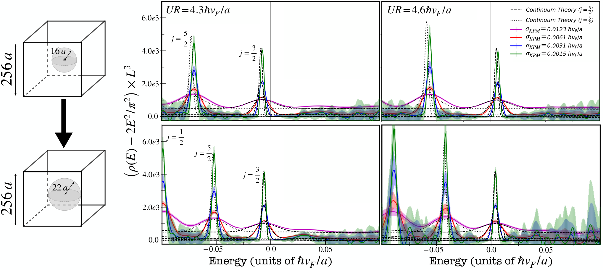
The first assumption to be tested is that internode coupling is irrelevant for the problem of spherical scatterers. Even though this is a very sound assumption provided the spheres are large compared to the lattice spacing , we still test it by evaluating the DoS deformation caused by a single scatterer of radius in a lattice with side . The calculations of the DoS were done using the KPM with a Jackson kernel, as described in Appendix 7, within implementation provided by the QuantumKITE [238], and using averaging over twisted boundary conditions to eliminate the mean-level spacing. As referred before, this numerical technique introduces a finite energy resolution by effectively broadening every energy Dirac- into a gaussian of variance , where is the number of Chebyshev polynomials retained in the expansion. Therefore, in order to compare our numerical results for the DoS with the analytic ones (obtained from the FSR), we convolute the latter with a gaussian that accounts for this finite spectral resolution, i.e.,
| (340) |
More precisely, we are interested in comparing the DoS deformation obtained from Eq. (324), with , to the results obtained for a single spherical scatterer of radius . Thus, the right quantity to represent is not the full numerically DoS but rather
| (341) |
This is to be compared with
| (342) |
that is the analytical FSR result for a single impurity of radius and potential , already broadened by the finite resolution determined by .
Some illustrative results are shown in Fig. 24, where it is clear that as becomes larger (e.g. ) the several resonances become well described by the continuum theory developed in the previous sections. In fact, we can even go further and exploit the finite resolution of the KPM calculation to analyze the DoS deformation caused by a critical spherical scatterer. In Fig. 25 a, we present these results for and a radius of , which are then compared to gaussians of width centered at the nodal energy. To the available resolution, an exactly critical impurity introduces zero energy bound states in the system, as predicted from our earlier. exact solution of Weyl hamiltonian.
In summary, we have established that, even in the more realistic lattice WSM with several nodes in the fBz, the structure of resonances predicted by the FSR for an isolated spherical scatterer within a single-node continuum model are well reproduced if the latter are sufficiently large. This is hardly surprised, as a slowly-varying potential in real-space is not able to induce scattering processes with large momentum transfer (see Suzuura and Ando [255] for a paradigmatic example).

Dilute Limit Hypothesis:
The numerical results clearly point to a great accuracy of the continuum theory to describe DoS’s deformations caused by isolated spherical scatterers. The only requirement is that the corresponding lattice perturbation is a smooth region significantly larger than the lattice spacing. However, the validity of the single-region theory is not enough to validate our earlier conclusions; We must also check that there is a well-defined dilute limit associated to this model of disorder. Even though such a result can be somewhat expected for a system with impurities that lie very far from each other, there are known examples [256] of systems in which the DoS is a non-analytic function of the impurity concentration. Therefore, this dilute limit assumption must be explicitly verified for our system of interest.
In order to show that, we have performed KPM simulations fo large systems () in which a set of spheres of radius were scattered, using the method described in Fig. 25 c. In analogy to Sect. 15, we considered several random configurations of scatterers and considered random values of , which have been drawn out of a gaussian distribution centered around the “magical value” , with a standard deviation . The results are shown in Fig. 25 c and fully confirm the DoS deformation predicted from the continuum theory in Fig. 23 a. In fact, by analyzing the mean nodal DoS, our results further confirm that a linear scaling with concentration, i.e. , exists in samples containing to random impurities per unit volume. These results confirms that our earlier dilute limit assumption makes sense in this context.
Chapter 4 Rare-Event States of Point-Like Impurities and Small Clusters
Chapters 2 and 3 gave us two examples of how different disorder types can result in distinct effects on Dirac-Weyl semimetals. First, the electronic DoS was analyzed in the presence of an Anderson random potential. Both the analytical and numerical calculations revealed that the semi-metallic phase, with a vanishing nodal DoS, remains stable up to a critical disorder strength, after which the DoS takes on a finite value. This corresponds to a non-conventional disorder-induced SMMT [209, 25, 192] that long precedes the conventional Anderson MIT. Afterwards, we also considered the case of a DWSM that is “decorated” by a finite concentration of sizable scalar spherical scatterers of random strength. This disorder model intends to mimic random smooth potential regions that can rarely appear within a disordered landscape. These "rare regions" are deemed relevant in the disordered semimetal phase because they are expected to create a finite density of states at the node, by means of a non-perturbative effect [32, 34, 37]. In this case, we have concluded that, as long as there is a non-zero probability density for these scatterers to support bound states, the nodal DoS gets lifted proportionally to their overall concentration in the system. Note that our conclusions for the latter model stand in stark contrast with our findings for the Anderson model, even when considering our unbiased simulation results.
The two disorder models analyzed earlier are obviously probing very different limits of what a disordered DWSM is. This partially justifies the contrasting physical effects but, as reported by Pixley et al. [34, 220], both the mean-field and the rare-event contributions (AQC) to the nodal DoS can be actually produced by the same type of disorder. In effect, if we have a random scalar potential with a local distribution that has unbounded tails 5656 56 Note that the numerical study of Chapter 2 dealt only with a local box-distribution potential. (such as a gaussian or a Cauchy distribution), the DoS shows a clear semimetal-to-metal transition at finite disorder, but its nodal value will remain finite — — even within the semimetal phase. From our simplified model of random scatterers, it is not possible to understand why does an “unbounded” Anderson potential yield an enhanced AQC effect, when compared to the bounded case (analyzed in Chapter 2). Understanding this enhancement is the main subject of this chapter, which will culminate in an alternative interpretation of what a rare-event of a disordered landscape really is. For that, we will begin by reconsidering the model of Chapter 3 in the limit of a vanishing scatterer radius (what we shall call a point-like impurity). Considering a continuous and lattice version, we will demonstrate an essential difference relative to the model treated in Chapter 3: bound states do not arise from a single point-like impurity but, instead, require a fine-tuned configuration of (at least) a pair of nearby impurities. Then, we will return to the disordered lattice WSM and use Lanczos Diagonalization (LD) to assess the appearance of rare-event nodal eigenstates in different random on-site disorder models, pinpointing the crucial role played by large fluctuations in the local potential. Finally, these rare-event nodal states in a disordered lattice are interpreted, not as being due to large smooth regions in the landscape (as claimed in Ref. [32]), but rather due to very small clusters of nearby sites, in which the conditions for a collective bound state are sporadically met. Some results presented here are original but still unpublished.
17 - Impurities in a Continuum Weyl Semimetal
In Chapter 3, we have shown that a spherical scatterer can create nodal bound states of Weyl electrons, if and only if the product of the potential () with its radius () takes on a fine-tuned discrete value. This condition becomes problematic in the limit , which drags all the “magical values” of to . Therefore, in order to study the problem of point-like impurities in the continuum, we follow the study of Buchhold et al. [37] and consider the perturbed single-node Weyl Hamiltonian,
| (343) |
(the same as in Sect. 8), but now with the perturbation
| (344) |
which is a simple sum of scalar -impurities. Unlike the spherical scatterers, these point-like impurities certainly generate scattering with arbitrarily large momentum transfer which would, in principle, invalidate the assumption of independent Weyl nodes in a lattice model. In spite of this, we can carry on with the continuum calculation and try to compute the eDoS for a given configuration of -impurities. To do this, we will take advantage of the reduced support of the perturbation (provided is a relatively small number) and employ a projected Green’s function method.
17.1 Projected Green’s Function Formalism
Obtaining the single-particle properties of the Hamiltonian in Eq. (343) is a standard problem in which we have a separable Hamiltonian, , about which we know everything in the absence of . To be more precise, we know from Sect. 8 the clean model’s SPGF 5757 57 All propagators here-forth will be considered as retarded, by default.,
| (345) |
where and a summation over is implicit. In the presence of any perturbation, the system’s SPGF encapsulates all single-particle properties of the perturbed system and has a completely analogous expression:
| (346) |
However, in practice, the matrix-inversion implied by Eq. (346) is not feasible and one must take some type of approximation scheme, e.g., perturbation theory, or use some clever trick that allows one to bypass the full inversion in the whole Hilbert space. Here, we will take the latter approach and, for that, we start by writing down the exact Dyson relations,
| (347a) | ||||
| (347b) | ||||
where stands for a full contraction of all indices/coordinates in the working representation. This pair of equations may be combined and written in the different, but equivalent way,
| (348a) | ||||
| (348b) | ||||
where is the (retarded) -matrix, an energy-dependent operator associated to the whole perturbation . Now, we bring about the essential point of the Projected Green’s Function (pGF) method: Both and only act non-trivially in a very restricted real-space volume, the support of the perturbation, which we generically call 5858 58 Note that, since we are dealing with single-particle problems, it is entirely equivalent to think about as small subset of real-space, or a very small subspace of the full system’s Hilbert space. and that, in our case, is composed by the positions where the -impurities are centered. This locality property of allows us to solve Eqs. (348a)-(348b) as a two step process:
- 1.
Project the system of equations into , i.e., given any general operator , and considering the projector onto the subspace of as the operator , we must transform in all equations. For the Green’s function equations, this yields
(349a) (349b) where we have used the fact that and . Clearly, Eqs. (349a) and (349b) form a closed set of coupled equations that can be solved explicitly. More precisely, we have
(350) and, consequently,
(351) Note that in the previous equations, contrary to Eq. (346), the matrix-inversion is not a problem because the matrices involved have small dimensions. For the specific case of the single Weyl node, solving Eq. (351) would involve the inversion of a dense complex-valued matrix. In a common laptop, one can numerically invert an complex dense matrix in less minutes and using about Gb of RAM memory for . Typically, these -based inversion algorithms scale as in CPU-time and in memory usage.
- 2.
The perturbed SPGF for any two points outside can be reconstructed from the perturbed one by using Eq. (348a), with the -matrix calculated in the previous step.
Note that all this process takes for granted that one knows, a priori, the unperturbed SPGF in real-space. If we know this quantity, then the aforementioned - matrix can be calculated as follows,
| (352) |
where , and where we have assumed a real-space representation that orders the basis of the projected subspace as
| (353) |
In summary, in the presence of a finite number of -impurities, the perturbed SPGF between any two points in space can be entirely determined by calculating the matrix presented in Eq. (352). The algorithmic complexity of this method comes from two stages: (i) the construction of the matrix to be inverted [an process], and (ii) the inversion of this matrix. As we shall see, this can be done analytically if the number of impurities is sufficiently small, namely .
Density of States and the Projected -Matrix:
The perturbed propagator between any two positions can be reconstructed from the knowledge of in the projected real-space representation of Eq. (353). However, for the purpose of calculating changes induced by in the system’s global eDoS it is hardly necessary to do that. The change in the eDoS is defined, in terms of SPGF as 5959 59 The global sign would appear reversed for advanced SPGFs.
| (354) |
where the trace is over the whole Hilbert space. Using the result of Eqs. (348a) and (351), we can cast this expression into the apparently more complicated form,
| (355) |
or, equivalently,
| (356) |
where we have used the cyclic property of the trace. Since both the rightmost and leftmost operators inside the trace have support in , one is entitled to replace the full trace by one that is restricted to this subspace, i.e.,
| (357) | ||||
where we have also used the fact that . Finally, we arrive at the essential formal result of this section: the change in the eDoS due to a cluster of -impurities can be obtained as a projected trace involving the projected -matrix and the clean SPGF. Although the form of Eq. (357) is the most useful for numerical calculations, it is worth remarking that there are alternative ways [37] of writing this result, namely,
| (358) | ||||
| (359) |
where use was made of the general matrix identity,
17.2 Bound-States and the Projected Lippmann-Schwinger Equation
Before moving on to calculate the eDoS deformation for particular cases, it is important to take a small detour and establish a further formal result. Here, we will show that the projected formalism can likewise be used to identify nodal bound states in systems of a few impurities. To see this, we start by writing the wavefunction equivalent of Eqs. (347a)-(347b); the so-called Lippmann-Schwinger Equation (LSE) [257, 258] for a scattering state ,
| (360) |
where is an eigenstate of the unperturbed system described by , being a parent extended state of . Note that Eq. (360) is an exact self-consistent representation of a solution to the perturbed quantum eigenvalue problem, and has the trivial interpretation that a perturbed solution can be seen as an unperturbed propagating wavefunction, at that energy, to which a scattering part is added. In principle, this equation also works to find non-propagating solutions, for which there is no parent eigenstate of the clean Hamiltonian, i.e.,
| (361) |
where is the energy of the state. Note that the previous equation clearly indicates that such a solution must belong to the kernel of the operator . Furthermore, if the perturbation has a finite support , one can project Eq. (361) into this subspace and get
| (362) |
where is the restriction of to the support . Remarkably, by analyzing the dimension of the kernel of , one can obtain possible bound states generated by the perturbation . To prove that such a state is a bound state of the system, it is necessary to reconstruct the corresponding wavefunction outside , that is,
| (363) |
where is an arbitrary position. Being a bound state or not then depends on the asymptotic properties of the clean SPGF in real-space. For this system any solution of Eq. (362) with a non-zero energy will not lead to a square-normalizable wavefunction, because . However, if we focus only on the nodal energy (), the reconstructed wavefunction is guaranteed to be normalizable by the property, 6060 60 Despite being a fairly common situation, there is no fundamental reason for a proper bound state to appear at energies where the clean system has a vanishing DoS. In fact, bound states within a continuous spectrum [259] are known to exist since the dawn of quantum mechanics (see the seminal paper of von Neumann and Wigner [260]).. Therefore, obtaining the null-space of the projected operator allows us to pinpoint the existence of many-impurity nodal bound states.
17.3 The Single- and Two-Impurity Problem
At this point, we have developed all the necessary formalism to study the spectral effects introduced by a set of -impurities in a Weyl semimetal. Here, we employ it for the analytical study of two important cases:
| (364) |
which describe a system of a single or an isolated pair of -impurities. These problems have already been addressed in Ref. [37] but are still of great importance to understand some major qualitative features of point-like scalar impurities in Weyl system. Namely, we will show that nodal bound states can only arise from quantum interference between several -impurities, unlike what happened with the spherical scatterers of Chapter 3.
The isolated -impurity case:
We begin by the perturbation, which is controlled by a single real-valued parameter, , measuring the strength of the local potential. Note that has dimensions of energy times volume, because the Dirac- is a 3D distribution. Considering the clean SPGF of Sect. 8, together with the “smooth cut-off” UV-regularizer considered there, we can explicitly write the -matrix as
| (365) |
where , is the smooth cut-off scale and is a matrix defined in a support of dimension . Hence, we have the following expression for the correction to the eDoS,
| (366) |
where is the eDoS measured in units of , while and are dimensionless parameters. In Fig. 26, we plot for different values of , demonstrating that a sharp resonance appears in the valence (conduction) band as (). This behavior is qualitatively similar to what was found for the spherical scatterers of Chapter 3 but with a crucial difference: the resonance never crosses the node. In fact, we can prove that there are no parameter able to generate a bound state of the -impurity, because
| (367) |
only has a single solution
| (368) |
which for zero energy (), cannot be satisfied by any finite .
Pair of -impurities distanced by :
In considering the two-impurity perturbation, , it is important to first realize that the continuum model is isotropic in space. This means that can be chosen to point in an arbitrary direction, e.g., , with no loss of generality. With the later choice, the -matrix associated to this pair of -impurities simply reads,
| (369) |
which, after some lengthy algebra, yields the following result:
| (370) |
where and are dimensionless quantities. From Eq. (370), we can obtain the correction to the eDoS due to the pair of -impurities, which we plot in Fig. 27. Before commenting on general results, we remark that the limit of Eq. (370) yields the additive result,
| (371) |
thus confirming a well-defined dilute limit for point-like impurities. Going back to the plots of Fig. 27, we can identify two distinct situations. If , the isolated impurities would lead to two resonances in either side of the node, which hybridize as they get closer together and are repelled away from the Weyl node. On the contrary, if , the two isolated resonances would be on the same band and hybridization tends to drive one of them towards the node until it crosses it. When this happens, the situation becomes analogous to the one described in Subsect. 14.1, and a non-degenerate nodal bound state is formed between the impurity pair. This argument can be proven directly by analyzing
| (372) |
Assuming zero energy, this determinant is null if and only if
| (373) |
which is -parameter fine-tuned situation. Note that, for the case presented on the left (central) panel of Fig. 27, we have a critical separation of (), which is consistent with the point at which the sharper resonance traverses .
The Role of Impurity Correlations:
At this point, we can already draw some interesting conclusions about the point-like impurity limit of the problem treated in Chapter 3. In this case, an isolated scalar impurity is not able to bind Weyl electrons at the nodal energy, independently of how strong the potential is. As one takes the impurity potential to more extreme values, an ever sharper impurity-induced resonance is observed to approach the Weyl node without ever crossing it. In order to have such a crossing, and the formation of a nodal bound state, it is crucial to include interference effects between two such impurities, as previously noted by Buchhold et al. [37]. However, even in this case the bound states are delicate and require three independent parameters to be fine-tuned: the impurity strengths and the distance between the two -impurities.
18 Atomic-Sized Impurities in a Lattice Weyl Semimetal
We have started by analyzing the case of point-like impurities in the single-node continuum model of a Weyl semimetal. By doing so, one is also taking for granted a set of assumptions that may not hold in the context of a lattice system and, therefore, require confirmation by analogous lattice calculations. In this section, we take the clean simple cubic lattice model given by the Hamiltonian,
| (374) |
whose properties are fully explored in the Appendix 10. Since this model is discrete, the -impurities of the continuum model must be replaced by a set of atomic-sized perturbations, such as,
| (375) |
where the potential takes the form,
| (376) |
Unlike the continuum case, here the s have dimensions of energy and, therefore, can be naturally measured in units of . Fortunately, this case is not fundamentally different from the one treated in Sect. 17, as all the pGF formalism may be directly translated into the discrete theory, without significant adaptations. The sole major difference will lie in the form of the real-space SPGF (usually called a lattice Green’s Function (lGF) in the tight-binding context) which will differ from the continuum one, and needs to be evaluated.
18.1 The Lattice Green’s Function
The first step to analyze the lattice problem is to calculate the lGF associated to the model of Eq. (374), something that can be easily done in -space, where
| (377) |
is the Bloch Hamiltonian, with being a vector of Pauli matrices and . Upon inversion of this Hamiltonian, we can obtain a general expression for the (retarded) lGF, in terms of an integral over the cubic fBz:
| (378) | ||||
which can be simplified by introducing a dimensionless energy, , a dimensionless position, , and a dimensionless crystal momentum, . This then yields
| (379) |
where the integral is now over the 3D cube, . The expression of Eq. (379) can be suitably divided into two fundamental parts, which must be treated independently, i.e.,
| (380) | ||||
or, equivalently,
| (381) |
In the form of Eq. (381), it becomes evident that the calculation of the lGF for this model reduces to the calculation of two constitutive (dimensionless) triple-integrals,
| (382a) | ||||
| (382b) | ||||
which are to be taken in the limit . Note that, in a simple cubic lattice, the vector is composed by a set of integer numbers and, due to cubic symmetry, the integral of Eq. (382b) does not depend on the index . In Appendix 10, we detail a semi-analytic procedure by which one of the -integrals in both Eqs. (382a) and (382b) can be performed analytically with the limit taken formally. By numerically performing the two remaining integrals, we are able to evaluate the lGF of the model to an arbitrary energy resolution. In Fig. 28, we show these results and compare them to the continuum limit near the nodal energy. As can be seen, the two models agree in the limit and , as they should.

Small-Scale Properties of the lGF:
Before using the calculated lattice Green’s function within the pGF formalism to study atomic-sized impurities in this lattice model, it is important and useful to comment on some special featured of that happen at the scale of the lattice spacing. More precisely, we can show that given a lattice displacement , the constitutive integrals are (i) all zero if two or three integers are odd, (ii) only is nonzero if all integers are even and, finally (iii) if and only if is odd, with the other two being even. This weird property is clearly a feature of the discretized model 6161 61 One can show that this actually comes from the destructive interference of excitations from Weyl nodes at different TRIM (see Appendix 11 for further details). and does not survive any coarse-graining procedure that leads to a continuum limit. Nevertheless, one must be aware of this non-universal property when making calculations in the lattice model, e.g., two atomic-sized impurities in the lattice model may be uncoupled due to a vanishing lGF between their positions.
The Case of Zero Energy:
Besides the aforementioned features at the scale of the lattice spacing, the lGF also features important symmetries referring to the reversal of sign in the energy. Concretely, we have
| (383a) | ||||
| (383b) | ||||
where we employed the transformation on the integrals of Eqs. (382a)-(382b). These symmetries imply that lGF obeys the following relation,
| (384) |
At zero energy, , Eq. (384) demonstrates that only the second term in the lGF survives, that is,
| (385) |
where the fact that is purely imaginary was also used.
18.2 The Single- and Two-Impurity Problem in the Lattice
After calculating the lGF between any two positions, we can now retrace the whole study of Subsect. 17.3, made for -impurities in the continuum model, and now check how it translates to a lattice model that has a built-in ultraviolet scale () and several Weyl nodes are coupled by point-like perturbations in real-space.
Apart from small-scale peculiarities which are inherited from the properties of the clean lGF, the conclusions obtained by considering one or two atomic-sized impurities are essentially the same as what we have seen for the continuum model. Namely, (i) an isolated lattice site with a scalar potential does not generate nodal bound states, giving rise to sharp resonances that get closer to the nodal energy as , and (ii) a pair of impurities (distanced by in the lattice and having potentials /) can create a nodal bound state by means of coherent scattering between them. Three representative examples of the eDoS change caused by a pair of atomic-sized impurities in the lattice are presented in Fig. 29.
In Fig. 29a, we show the calculation done for two points with local potentials that have the opposite signs. Just like the continuum -impurities, effects of hybridization act to further split the resonances and drive them farther from the nodal energy. In Figs.29b and c, an analogous calculation is presented but now with impurities that have . In this case, we find two seemingly different situations; If has only even coordinates, the two resonances hybridize only slightly at short distances but there is not peak being driven towards the nodal energy. In contrast, if one is odd, the two resonances hybridize strongly such that one of the resonances is driven through . The difference between the two cases lies on the fact that only the latter case has a nonzero prefactor for the term . Therefore, we conclude that the latter term is the one ultimately responsible for creating nodal bound states through inter-vacancy interference. Finally, it is worth noting two further points: (i) that, in all the cases, the impurities do not hybridize if has two or three odd coordinates, and (ii) that the limit of this exact lattice calculation always coincides the analogous calculation within the multi-valley continuum approximation derived in Appendix 11.

18.3 Minimal Clusters for Nodal Bound States
The same analysis that was done for two points in the lattice WSM can also be repeated for an arbitrarily complex cluster, with each point having its own local potential. From the discussion of Sect. 17, we are already aware that increasing the complexity of the cluster of point-like impurities entails a very unfavorable scaling of the method, as a larger matrix is required to be numerically built and inverted. Therefore, we will focus on the simple case of very small clusters of adjacent points in the lattice, as shown in the scheme of Fig. 30.
Our main point here is to push the theory of smooth regions, as presented in Chapter 3 to its small-size limit, i.e., examine the possibility for a small cluster of adjacent site with the exact same local potential, , to give rise to nodal bound states. In the plots of Fig. 30, we present results for the change in the eDoS as a function of for three types of clusters: a line of three sites, a planar cross along the -plane, and a three-dimensional cross. In all the cases we see there is a sharp DoS resonance that is driven through the nodal energy as is increased 6262 62 We have considered only positive potentials, with no loss of generality.. When such crossing happens, at a critical value , there is a nodal bound state that forms akin the ones that were observed for the spherical scatterers in the previous Chapter. In fact, the latter will be obtained as the limit of these results when the radius of the cluster considered becomes sufficiently large. An important feature of these critical values is that they become smaller as the cluster includes a larger number of sites, as illustrated in the scheme of Fig. 30.
19 What are Rare-Regions in a Disordered Lattice?
Now, we are ready to establish a connection between the mesoscopic view of nodal bound states, undertaken in previous sections, and the rare-region-induced effects that were numerically found by Pixley et al. [34], leading to an AQC scenario for the mean-field transition in disordered WSMs. For that purpose, we take a step back and carefully analyze what these non-perturbative effects really are in the context of a disordered lattice. To do this, we numerically study the nodal eigenstates of disordered WSM lattices (of side dimension ), using the implicitly restarted Lanczos diagonalization algorithm [261, 262], as implemented in ARPACK [263]. In order to separate any putative nodal bound state, from the extended Bloch-like states, we employ twisted boundary conditions (with fixed twist of rad in all directions) to open up a finite-size gap, , inside of which the rare-region-induced states will lie. We recall that this segregation is due to a greater degree of localization expected for the rare-region-induced states which, as pointed out in Ref. [34], makes them much more insensitive to the boundary conditions than the extended ones. Finally, we remark that a similar analysis was undertaken by Pixley and Wilson in Ref. [220]
In Fig. 31, we present results from diagonalizing independent samples of the (squared) disordered Hamiltonian, . For reasons that will become clear, we considered two different models of uncorrelated scalar disorder that differ solely on their local potential distributions:
| (386) |
i.e., a box-distribution (BD) and a gaussian distribution (GD). Note that, in both models, the parameter measures the strength of disorder in a comparable way, that is, for a given both local distributions have the same standard deviation. For the two models, and several values of 6363 63 All chosen below the mean-field critical disorder., we plot in Fig. 31 the four lowest (absolute) eigenvalues of all samples, in succession. Simultaneously, we also show (in the left panels) a scatter plot of the corresponding Inverse-Participation Ratios (IPRs) [223, 264, 207] of each determined wavefunction, i.e.,
| (387) |
which characterizes the degree of locality of a quantum state in real-space thus allowing one to correlate the eigenenergies with the localization of the corresponding eigenstates. This quantity is perhaps the simplest way to distinguish between localized and delocalized quantum states: one expects an extended three-dimensional Bloch-like wavefunction to have , while for a localized one. Notice that the scaling with which is presented in Fig. 32b for the data obtained with the GD model further confirms the interpretation of the rare-region-induced states as localized (or quasi-localized), while the ones belonging to the energy strips are likely extended.

For the BD disorder model, we observe that the only effect of disorder is to randomize the clean energy levels into “energy strips” that get wider () and approach the nodal energy () as increases (scalings are demonstrated in Fig. 32 a). Actually, this is the expectation obtained from the - order perturbation theory presented in Appendix 12, and the values of the IPRs further confirm that all these states are indeed extended. In great contrast, the GD model generates a behavior that is qualitatively very different; Besides having the same energy strips of Bloch-like states that behave identically to the BD case, there are also a different class of “rarer states” with energies that clearly invade the finite-size gap, . These states, which have IPRs orders of magnitude higher than the ones in the energy strips, are the rare-region-induced eigenstates that create the exponentially small background DoS in the numerical results of Ref. [34].

19.1 The Role of Unbounded Local Distributions
Recapping the numerical results presented at the end of Chapter 2, we have not seen any signs of AQC in spite of having pushed the limits of our KPM simulations in both system size and spectral resolution. The previous analysis of the Anderson BD model makes it clear why no rare-region-induced effects could be observed: because, statistically speaking, there were none! As a matter of fact, it had already been pointed out, in Refs. [34, 220], that one must consider disorder models with unbounded local distributions for allowing the rare-region-induced AQC to appear in lattice simulations. In more direct terms, we can state that, while the mean-field criticality is driven by the disorder strength parameter, the rare-region effects depend on large fluctuations on the disordered potential.
One outstanding question that we can legitimately ask is the following: How many rare fluctuations do we need to generate the rare-region induced states? To answer this question, we repeat the analysis of the BD disorder model, but now with an additional fixed isolated potential spike, of strength , that is placed by hand in all the random samples. In Fig. 32 c, we present these results where it becomes clear that high-IPR in-gap states start to emerge immediately, in way that is very similar to what was obtained for the GD model. Therefore, the short answer to our previous question is simply: one. This surprising conclusion contradicts the picture advocated in Nankishore et al. [32], according to which the AQC in a disordered WSM is caused by bound states of rare smooth regions in the potential landscape. Statistically speaking, there are roughly as many smooth regions in the GD (or the BD + fluctuation) disorder model, as there were in the BD Anderson potential of Fig. 31. Notwithstanding, no rare-event eigenstate could be detected in the latter case. Thereby, we may conclude that these rare-event states are better interpreted as being fine-tuned bound states that emerge from the coherent scattering of two (or maybe more) nearby lattice points, which can have very asymmetric local potentials. This is precisely a realization of the mesoscopic mechanism unveiled in Subsect. 18.2, which singles out the isolated large potential fluctuation as a “nucleation center” for bound eigenstates to appear by interference with the (much weaker) surrounding disorder.
20 A Consistent Picture of AQC in a Lattice Model
From our study of the nodal eigenstates at the mesoscopic level, we have pinpointed two main mechanisms by which these can emerge from an uncorrelated disordered potential. On the one hand, we have a Two-Point Asymmetric Interference (2PAI) mechanism, by which an isolated large fluctuation of the disordered landscape hybridizes with one (or more) of its neighboring points generating states as the ones described in Subsect. 18.2. On the other, we have a Minimal Smooth Cluster (MSC) mechanism, which is akin the rare-region mechanism of Chapter 3, but which we have shown to require very minute clusters of nearby points in a lattice.
Within an arbitrary disordered landscape one expects both the 2PAI and the MSC mechanisms to generate nodal bound states and, thus, avoid the mean-field quantum critical point in these systems. Nevertheless, if the local disorder distribution happens to be bounded, the system may find itself in a situation where the 2PAI mechanism is actually absent for weak disorder, as there may be impossible for two nearby fluctuations to meet the criterium for the emergence of a joint nodal bound state. In principle, the MSC mechanism is always possible for arbitrarily weak disorder. However, as the disorder strength gets decreased, the size of the smooth clusters must grow accordingly in order to bind nodal electrons. Such large smooth regions are extremely unlikely for uncorrelated disordered potentials which ultimately explains why we could not observe any signs of AQC with the BD Anderson disorder.
Chapter 5 Vacancies in Weyl Semimetals
In Chapters 2 to 4, we have addressed the effects of disorder in the spectral properties of emergent three-dimensional Weyl fermions near the Fermi level of a quantum solid. For that, we analyzed three different models of quenched disorder (uncorrelated random potentials, randomly placed smooth regions, and scalar point-like impurities) in the context of continuum single-node models, as well as multi-valley lattice models. While these simple disorder models yield some interesting (and somewhat surprising) effects, they do not describe all the sources of disorder one finds in actual crystalline samples that are grown in the laboratory. Usually, even the most perfect crystals suffer from poor stoichiometry or flaws in the crystallization procedure [265, 266], that give rise to substitutional disorder (atomic impurities), lattice imperfections (e.g., missing atoms [267] or deformed unit cells), inhomogeneous strain, or other topological defects [68, 268]. Adding to all of these, real samples will often be multi-crystalline and always have some vibrational dynamics due to thermally excited phonon modes [269, 270]. All in all, these effects break the lattice translation symmetry, which will scatter the propagating Bloch electrons, and may significantly change the electronic properties of the material [271].
By this point, we will consider another common type of lattice disorder which is due to be present in real samples: dilute lattice vacancies. Vacancy-disorder in a tight-binding Hamiltonian corresponds to a set of randomly chosen orbitals that got removed from the system 6464 64 And, therefore, also from the single-electron Hilbert space.. Such a procedure attempts to model the effects caused by isolated atoms that are missing from the crystal [272, 267], but without accounting for the more complicated lattice distortions and charge screening which are also expected to appear around the vacant site [273]. Even so, the simplest models of random vacancies (also called point-defects) are able to generate novel and remarkable physical phenomena that can serve to explain real experimental results. Graphene is a prime example of how point-defects can give rise to fundamentally different physics that goes far beyond what can be reproduced by Anderson random potentials. There, random vacancies effectively realize a chiral-symmetric (see Sect. 3) disorder model [274] which originates robust nodal bound states that greatly enhance the density of states at the charge neutrality point [62, 26], and lead to a finite universal dc conductivity [42, 256]. Regarding three-dimensional semimetals, the influence of vacancies have been overlooked so far in theoretical literature, even though these are common sub-products of the synthesis process [275] and have even been experimentally observed by Transmission Electron Microscopy (TEM) in stoichiometric Weyl semimetals [276]. Additionally, the concentration of vacancies may also be externally controlled by means of light-ion irradiation of a crystalline sample [277]. While being still an unexplored territory, the study of vacancy effects in these systems has recently received a motivational boost by the experimental results of Xing et al. [278], that established a link between surface vacancies in the magnetic WSM, , and the existence of exotic localized Spin-Orbit Polarons. In this Chapter, we will present novel results on the effects of diluted vacancies in a cubic Weyl semimetal focusing, not only on the spectral effects, but also in predicting observable signatures in dc transport, magnetic response and optical properties. This original study is published in Refs. [2] and [3].
21 Modeling a Vacancy in a Weyl Semimetal
Before analyzing the case of a finite concentration of vacancies in a macroscopic sample, we begin by considering the simpler problem of an isolated vacancy in the tight-binding model of a cubic WSM, which was first introduced in Eq. (276). Our clean Hamiltonian reads
| (388) |
where is a simple cubic lattice of parameter , are the cartesian unit vectors, are local two-component fermionic creation/annihilation operators, and are Pauli matrices. In this model, a vacancy defect is a missing lattice site, which can happen in two ways within the two-band Hamiltonian of Eq. (388): (i) by removing all atoms in a unit cell (a full-vacancy), or (ii) by removing only a single orbital (a half-vacancy). In a bipartite lattice, like a graphene monolayer, this choice is clearly important due to the sublattice symmetry, which is broken by a concentration imbalance between the vacancies in each sublattice [274]. However, here the situation is less symmetric because does not have a sublattice symmetry to begin with 6565 65 A 3D Weyl semimetal is not chiral symmetric, which is obvious from the matrix form of the corresponding Bloch Hamiltonian.. Therefore, we shall only treat the case of a full-vacancy, keeping in mind that no new phenomena would arise if half-vacancies were considered instead 6666 66 This was explicitly verified in Santos Pires et al. [3], and can be easily obtained from the same pGF method that will presented in the remainder of this section.. Under this framework, a single full-vacancy is implemented by removing the hoppings connecting both orbitals within a unit cell to the remaining lattice. This procedure actually leaves behind the disconnected site, something that we must take into account when looking at spectral properties. With no loss of generality, we start by considering the vacancy as placed at the origin () and, thereby, add to a term that precisely cancels all hoppings to this site, i.e.,
| (389) |
Note that the perturbation has the advantage of acting only on the finite support , which forms the octahedron depicted in Fig. 33. Such a local perturbation to a lattice model can be conveniently studied by using the whole machinery of the projected Green’s Function (pGF) method introduced in Sect. 17. To more easily apply the pGF formalism, it is convenient to encode the sites of in the order, , such that the single vacancy perturbation looks like,
| (390) |
i.e, a simple matrix in the projected subspace. In Eq. (390) (and following), we define as an zero matrix, as an identity matrix, and as a vector of Pauli matrices. At the same time, using the short-distance properties of the lGF and its symmetry around the nodal energy (derived in Subsect. 18.1), we also see that the projected lGF reads simply as
| (391) |
where , and are dimensionless functions of energy, that are determined from the integrals in Eqs. (382a)-(382b). To be more precise, we have
| (392a) | ||||
| (392b) | ||||
| (392c) | ||||
whose integrals, over the cube , can be performed semi-analytically in the limit (as described in Appendix 10). It is also relevant to emphasize that is a special point, in which the clean pGF takes on the particularly simple form,
22 Nodal Bound States of an Isolated Vacancy
The simple matrices defined in Eqs. (390)-(393) can be plugged directly into the expressions derived within the general formalism presented in Chapter 4, In particular, a first question that can be asked is whether or not a vacancy is able to create bound-states at the nodal energy. For that, we use Eqs. (390) and (393) to build the projected operator , whose determinant takes on the remarkably simple form,
| (394) |
The operator must have, at least, a two-dimensional kernel subspace because of the two orbitals that were disconnected from the lattice. Hence, with our implementation, a vacancy always produces a couple of “trivial localized states”, corresponding to the Wannier orbitals that were removed. However, what Eq. (394) is also telling us is that the kernel is actually four-dimensional. This implies that an additional pair of “non-trivial bound states” also appears, these extending into the remaining lattice. In fact, a full diagonalization of yields the following projected wavefunctions:
| (395a) | ||||
| (395b) | ||||
where are the local Wannier states ( labels the orbital). Upon a reconstruction of the states outside of the original support, , these yield the following wavefunctions:
where are spinor components of the lGF. Note that, from the continuum approximation derived in Appendix 11, Eqs. (396) and (396) imply that the new states generated by the vacancy correspond to square-normalizable wavefunctions in the lattice, with tails that decay asymptotically as . Both the existence of these states and their asymptotic behavior are confirmed by the Lanczos Diagonalization (LD) results presented in Fig. 34 a. Further discussion is left to the next section.
Deformation in the Density of States:
Since the dimension of the system’s Hilbert space was not changed, the presence of extra nodal bound states necessarily implies that some spectral weight was drawn out the band-continuum to the node, by the vacancy. To characterize this process, we assess the vacancy-induced deformation in the global extensive density of states (eDoS), through Eq. (357), and using the matrix expression of the clean lattice pGF at all energies, given in Eq. (391). Therefore, we obtain
| (397) |
where all the functions , and (and their derivatives) can be numerically calculated from Eqs. (392a)-(392c). A plot of is shown in Fig. 34 b, where we see that a negative correction to the eDoS appears across the entire band spectrum. This is consistent with an overall transfer of spectral weight to the emergent nodal bound states. Also, the integral of this curve is exactly , because the number of continuum states is not conserved, i.e., two states (per orbital) appear as vacancy bound-states while two others were removed from the Hilbert space.

23 Density of States With Multiple Vacancies
An isolated lattice vacancy produces a doublet of exact nodal bound states in our model of a Weyl semimetal. Under a dilute limit argument, a finite concentration of vacancies, , would give rise to an accumulation of nodal eigenstates per unit volume, which would change appreciably the electronic properties near the Weyl node, relative to the clean WSM case. However, as happened for the bound states analyzed in Chapter 3, these nodal states decay asymptotically as a power-law and, therefore, a strong inter-vacancy interference can potentially affect the results in the presence of multiple vacancies. To study this case, we now employ a combination of KPM and LD calculations to tackle the many-vacancy problem and see which features of the single-vacancy case would survive the more realistic scenario of a macroscopic number of vacancies.

Our starting approach is based upon a LD of lattices having unit cells, and containing a prescribed concentration () of randomly placed vacancies. As detailed in Appendix 8, the use of twisted boundary conditions opens up a finite-size gap in the spectrum that serves as a separation between the nodal bound states, and the extended ones. In principle, any state is affected by phase-twists at the boundaries of the simulated cell, but extended states will certainly be more sensitive. As in Sect. 19, our finite-size gap will work as an “energy bin” in which the vacancy-induced states lie and, thereby, we can simply ask the diagonalization algorithm to compute the eigenpairs 6767 67 Naively, one expects that each vacancy gives rise to two bound states, which makes this number sufficiently large to capture most states within the finite-size gap. that are closest to . In Fig. 35 a, we present a scatter plot of the energies and corresponding IPRs of every eigenpair determined for a set of random arrangements of vacancies, with a concentration that ranges from to (per unit cell). The results clearly demonstrate that, in spite of the proximity between vacancies, the system still features a large number of high-IPR eigenstates which are flanked by a region of extended states. This physical interpretation is further confirmed by Fig. 35 b, where a 3D bubble chart of is depicted for two eigenstates randomly chosen from each of the regions.
The study of inter-vacancy effects by LD can provide us with a qualitative picture on how the eigenstates near the Weyl node look like, in the presence of many vacancies. However, this approach is severely limited by the effective spectral resolution 6868 68 The main issue is that the Lanczos algorithm can miss eigenstates that are nearly-degenerate. In contrast, the KPM algorithm calculates observables that involve the entire spectrum, albeit with an artificial broadening of the individual energy levels., the finite number of eigenstates that can be considered, and the attainable system sizes, which precludes a clear physical picture of what to expect in the thermodynamic limit. Therefore, we now complement the LD results with full-spectrum simulations of the mean DoS based on the Kernel Polynomial Method (KPM), which is lengthly described in Appendix 7.
Average Density of States:
Our KPM results for the mean DoS are summed up in Fig. 35c, where we present an overview of the entire spectrum, for different vacancy concentrations. The plots show a big enhancement of the number of states in (and around) the nodal energy, which indicates that the nodal DoS gets quickly and strongly lifted as increases 6969 69 One can think of this as the limit of the results found for atomic-sized impurities considered in Sect. 18.. This effect is consistent with the prevalence of the single-vacancy nodal bound states at finite concentrations, and qualitatively agrees with what was concluded from our previous LD analysis. Nevertheless, as the central peak grows in height, a much wider symmetrical profile emerges at its base. This is a telltale sign that inter-vacancy hybridization, which becomes stronger for smaller typical distances between vacant sites, is turning the bound states of isolated vacancies into low-energy scattering resonances within the continuum. This, however, does not change the total number of vacancy-induced states around the Weyl nodes, sine the integral of the full central correction to the DoS is seen to be proportional to (see the inset of Fig. 36c). In the bottom panel of Fig. 35c, we present a closeup of this broadened central peak where, in addition of showing that the vacancy-induced spectrum is diffused around , we can also observe the emergence of a finer structure of subsidiary peaks (a comb of sharp scattering resonances) around the node for concentrations .
23.1 Inter-Vacancy Hybridization in 3D Weyl Semimetals
Our KPM results clearly demonstrate that inter-vacancy effects become relevant in determining the induced changes in the DoS. Simply put, isolated vacancies would place new (proper) bound states at the nodal energy, but a finite concentration of these defects actually translates into a broadened central peak in the DoS. This is hardly a surprising result, as one expects quantum-interference effects to becomes relevant in any system that hosts a sufficiently large concentration of impurities. What is surprising here is the appearance of a superposed comb of sharp subsidiary resonances at finite energies for . In Fig. 36a, we present a finer analysis of this structure as a function of . There it becomes evident that, prior to being washed-out, these resonance peaks move away from the node proportionally to the vacancy concentration. Moreover, we also show in Fig. 36 b an analogous calculation done in a two-dimensional version of 7070 70 A square lattice Hamiltonian which is the same as in Eq. (388), but restricted to the -plane., which realizes a (chiral-symmetric) 2D Dirac semimetal. Despite displaying a similar broadening of the central peak due to inter-vacancy effects, our results show no signs of a modulated structure of subsidiary resonances. The previous comparison between 2D and 3D analogous systems provides a clue on the nature of these resonances. Intuitively, one expects an increased dimensionality to decrease the quantum-interference effects. While 2D vacancy-induced states get rapidly driven away from the nodal energy, in 3D, the quantum-interference effects are reduced such that inter-vacancy hybridization happens through an intermediate phase with very sharp resonances around the node, that still preserve some degree of locality around one (or a few) vacancy(ies).

23.2 Magnetic Sensitivity of the Subsidiary Resonances
The claim of locality [Subsect. 23.1], done for states composing the subsidiary resonances, deserves some further attention. In fact, from the LD results presented in Fig. 35a, we have already some evidence that the many-vacancy states which accumulate around the nodal energy are rather localized. Looking at the highest IPRs shown in Fig. 35a, we see that these are way too big for the states to be extended near the node. However, it is not easy to numerically prove this statement, because the LD algorithm can yield artificial linear combinations of

nearly-degenerate eigenstates, whose IPRs would scale with in an extended-like fashion (i.e., ). This faulty behavior of the LD algorithm is illustrated by the 2D scheme shown in Fig. 38; There, we start with an well localized system for which an eigenstate is found using LD with a spectral accuracy . Within , there are exact energy levels such that the LD algorithm yields an artificial linear combination of three localized states and, thereby, a squared-wavefunction with three blobs in the simulated plane. If we now increase the system’s size from (without changing ), then additional exact levels will exist within the accuracy window and, therefore, the obtained wavefunction will have roughly four times the number of blobs as shown in the bottom panel of Fig. 38. This way, we can see that the IPR of such a state, despite the fact that it may have small nominal values for a fixed , will scale with the system size in precisely the same way as a typical extended state of that dimensionality.
Due to this limitation, we now change our strategy and attempt to better understand the hybridized states by directly calculating the DoS for a more controlled vacancy disorder model, in which a predetermined number of vacancies are positioned in the places of an underlying superlattice 7171 71 The spacing parameter of this superlattice is the mean distance between vacancies, as determined by their concentration, .. Then, the mean DoS is calculated using the KPM for a series of samples in which the (originally periodic) vacancy positions are randomized by a vector , where are independent random integers for each vacancy. In Fig. 37 a, we showcase the mean DoS using the above procedure to position the vacancies in the lattice. From our results, we see that an almost periodic positioning of the vacancies, even though it still causes a broadening of the central peak, does not create any additional structure in the density of states. However, as soon as becomes sufficiently large to allow two (or more) vacancies to be distanced on the order of , the structure of subsidiary resonances re-emerges. These results, though indirect, hint that these resonances can be interpreted as hybridized states of a few nearby vacancies (i.e., resonances of small vacancy clusters).
Magnetic Sensitivity:
By this point, the reader must be rather convinced that both the central peak and the subsidiary resonances in the mean DoS correspond to heavily localized states. The former are likely weakly perturbed single-vacancy states, whilst the latter probably correspond to hybridized states between a few nearby vacancies. Nevertheless, we do a further computation to support our earlier claim: We calculate the mean DoS with a finite concentration of vacancies

in the presence of a magnetic field along the direction.
As depicted in the scheme of Fig. 39, if a wavefunction is localized in real-space, then the effects of an applied magnetic field will only be appreciable if the corresponding magnetic length scale, , is small when compared with the linear spatial extension of the state itself. Therefore, a spectral region composed of more localized states is expected to be less sensitive to applied magnetic fields. Such a magnetic insensitivity have actually been observed near the nodal energy of a Weyl semimetal with gaussian white-noise disorder by Lee et al. [279], being attributed to the presence of rare-event bound states [like the ones shown in Fig. 32]. In Fig. 37 b, we illustrate such an effect in the mean DoS (cubic WSM lattice of side 7272 72 Under periodic boundary conditions and a typical lattice spacing of , this corresponds to a minimal field of .) as a function of the magnetic field strength , and with a fixed vacancy concentration . Clearly, the areas identified earlier as being composed chiefly of more localized resonances (shaded in the panel) are also the energies for which the DoS shows lesser sensitivity to the applied magnetic field. For completeness, we also show corresponding calculations done in the absence of vacancies (shown in the inset of Fig. 37b), which clearly place the system in a regime of well-defined Landau bands [280, 281] and a finite plateau in the DoS around the node, due to the dispersion of the lowest Landau level along the magnetic field direction (see Subsect. 7.1 for a detailed discussion of the Landau spectrum near a Weyl node).
24 Impact of Vacancies in DC and Optical Conductivies
So far, we have focused on static spectral properties of Weyl electrons under the influence of vacancy disorder. Concretely, we have characterized the changes that are induced in the mean density of states and further characterized the qualitative structure of the corresponding wavefunctions in real-space. With the advent of thin-films, two-dimensional materials and surface-state electronics, the single-electron density of states appeared as a quantity of great experimental interest in its own right [282], because its real-space value could be measured by Scanning Tunneling Spectroscopy [283, 284] (STM) or, in -space, via Angle-resolved Photoemission Spectroscopy [285] (ARPES). For the bulk DoS of a three-dimensional sample, direct measurements are generally not available and one must resort to indirect measurements, such as, low-temperature specific-heat [286, 287], electronic transport or optical response measurements. In this section, we present our own predictions of the effects cause by vacancy-induced nodal bound-states (and their hybridized counterparts) on the dc conductivity and linear optical response of a Weyl semimetal.
24.1 Longitudinal DC Conductivity
The first quantity we study is the bulk linear longitudinal dc conductivity, , which is phenomenologically defined as
| (398) |
where is the electric current density in the bulk, and is the applied static electric field. Note that this conductivity is a function of the Fermi energy and, in fact, it is a property of states lying at the Fermi surface. Therefore, provided has control over the value of , this is a natural quantity where to look for signals of both the enhancement of the nodal DoS, as well as the subsidiary resonances arising from inter-vacancy effects. In the diffusive transport regime, the conductivity is beautifully related to the density of states at the Fermi level through the well-known Einstein Relation,
| (399) |
where is the elementary charge, is the quantum electronic diffusivity at the Fermi level, and is the mean DoS at the Fermi level. Therefore, if the quantum diffusivity were not affected by the vacancies, all the features found in the mean DoS would be precisely reproduced in the conductivity as a function of . However, such an insensitivity of to the vacancy disorder cannot be true in the light of the localized nature of the states that are introduced in and around the nodal energy. In fact, as pointed out by Elattari et al. [253, 254], whenever sharp resonances appear in the DoS, there is a great possibility of a strongly suppressed quantum diffusivity at those energies. Such an effect could counteract the enhancement in the DoS and effectively reduce the conductivity.

In order to study this quantity accurately, we performed large-scale unbiased real-space simulations of the mean dc conductivity using the Single-Shot Kubo-Greenwood method implemented in the QuantumKITE software (and described in Appendix 7). Our results for are summarized in Fig. 40a for vacancy concentrations of and , in a lattice with side , and spectral resolutions in the range of . The results show that the dc conductivity, first decreases, but then grows steadily as the Fermi level gets driven away from the node (see gray lines in 40a). However, upon a closer inspection there is a more outstanding feature in the results: precisely at the energies where the subsidiary resonances appear, the conductivity displays dips relative to its overall background value. In Fig. 40a, we complement these conclusions by showing the effect of an increasing temperature (thermal broadening of the Fermi surface) in the conductivity. From these results we realize that, even though the conductivity dips cannot survive up to arbitrarily high temperatures, one is still expected to observe them at temperatures as high as .
Physical Mechanisms:
The overall growth of the dc conductivity away from the nodal energy is an expected result, that may be seen as the trivial effect of an increased density of states. In contrast, the physical interpretation of the aforementioned conductivity dips is a more subtle issue, which cannot simply be an effect of the DoS’s energy modulation. As a matter of fact, these can only be explained by considering that the quantum diffusivity is strongly suppressed at the subsidiary resonances which, in turn, is due to the localized nature of the states that compose them. This suppression is sufficient to reduce the overall dc conductivity, in spite of the larger number of states that exist at that Fermi level.
24.2 Linear Optical Response
We have seen that it is possible, in principle, to detect the vacancy-induced features of the mean DoS using bulk dc transport measurements in crystalline samples. To detect the described effects, however, an active tuning of the system’s Fermi energy is required. This is easily achieved in two-dimensional materials, where a back gate voltage may be used to alter the bulk charge carrier density. On the contrary, tuning the Fermi level of a 3D material is generally a much more complex process that employs relatively new experimental techniques, such as a electric field-effect in thin-films [288, 289], or a precise stoichiometric control during an epitaxial growth process [290]. For this reason, it is useful to turn our attention for alternative measurable properties that (i) are sensitive to the existence of vacancy-induced nodal states, and (ii) do not depend on modifying the Fermi energy of the system. The optical response coefficient is such a quantity, where the frequency of the excitation field () plays the role of an external control parameter that can be easily changed.
In order to assess the effects of vacancies in the optical response of a Weyl semimetal, we have evaluated the -dependent linear conductivity of the tight-binding model defined in Eq. (388), using the real-space approach developed by João et al.[291] and currently implemented in the QuantumKITE package[238]. This method is based upon the spectral expansion of the linear Kubo formula,
| (400) | ||||
where is the lateral size of the simulated system, is the disordered Hamiltonian, is the Fermi-Dirac distribution, is the velocity operator, , and are the advanced/retarded SPGFs of the system (in the presence of disorder). The numerical calculation of this quantity involves an intrinsic spectral resolution, , relative to which one must assure the convergence of the obtained results (numerical method detailed in Appendix 7).

In Fig. 41 a, we present numerical results obtained for the real and imaginary parts of in the presence of either vacancies, with concentration , or a random Anderson potential of strength 7373 73 Concretely, this corresponds to an on-site random potential with a box distribution of width . . For a pristine, but slightly doped WSM (), the vertical inter-band transitions are Pauli blocked if . This defines the system’s optical gap, in which the imaginary part of the optical conductivity is finite, but reverses sign at . Our numerical results clearly show that the optical response of the material gets altered by the presence of both types of disorder and, more importantly, that it can be used to establish a clear distinction between the two models (random on-site potential versus vacancies). With a random potential, the optical gap remains intact at weak disorder, with the transition being simply smoothened as is increased. In addition, we also see that the typical linear dependence of is changed by the disorder, showing a slope that increases with . Remarkably, in the presence of random vacancies, no major changes are observed in except for the appearance of a new optical gap at that initiates a plateau in for the interval . This distinctive features of vacancy-induced optical response is highlighted in Fig. 41b, where it is also clear that the change in sign of no longer happens at but at lower frequencies.
Physical Mechanisms:
By now, it became clear that the optical response of a bulk WSM containing lattice vacancies, displays very distinctive features that can be unambiguously connected to the presence of vacancy-induced nodal states. As a matter of fact, these features can be traced back to the macroscopic number of states that the vacancies introduce close to the nodal energy, and the fact that these are states which strongly deviate from extended Bloch states. As such, the vacancy-induced states efficiently participate in momentum non-conserving (but energy conserving) transitions to/from the extended states at the Fermi level. Since the vacancy states only occur for , these transitions give a contribution to the real part of the conductivity starting at . This interpretation also explains why the width of the transition to the vacancy-induced absorption regime indirectly probes the energy width of the central peak in the DoS and, therefore, also the extent of inter-vacancy hybridization. Above the clean system’s optical gap, the most relevant processes are the vertical transition between valence/conduction Bloch states. Since vacancies, unlike Anderson disorder, do not renormalize strongly their Fermi velocity, the slope of remains unchanged.
Chapter 6 Concluding Remarks and Outlook
Topological semimetals are well known for their unique electrodynamic properties, but also for their robustness to perturbations which are due to topological constraints. The topology of the band-structure guarantees, to some extent, that Weyl nodes will remain stable for a wide range of Hamiltonian deformations. However, it does not imply that physical properties of the emergent Weyl fermions will be unaffected by them. In this thesis, we studied the mechanisms by which different types of disorder can alter the basic properties of the nodal quasiparticles in a Weyl (or Dirac) semimetal. Our main focus was placed on the destabilization of semi-metallic phase which can be induced by disorder in these systems, and turns an incompressible gas of Weyl fermions into a fundamentally different diffusive phase characterized by a non-vanishing density of states. Thereby, the electronic mean density of states emerges here as the central physical observable that characterizes the disordered Dirac-Weyl semimetal, and which we compute in the presence of different types of disorder: Anderson on-site potentials, random spherical scatterers, scalar point-like impurities, and lattice point defects. By analyzing all these cases, we have concluded that disorder effects in these systems can show a very non-universal character which deems a model-by-model analysis important for interpreting the results of future experimental studies. Despite having focused mostly on the density of states in the presence of disorder, we have also assessed some more easily measurable quantities, such as the electronic specific heat, the dc conductivity, the electronic magnetic properties, and also the linear optical response. These studies are important since they, not only indicate where to look for relevant signs of disorder-induced phenomena in upcomming theoretical studies, but may guide the fundamental explanation of future experimental results.
Before moving onto the outlook of this work, we present a short description of what the purpose and main conclusions of each Chapter are.
Chapter 1:
A self-contained introduction is given to the physics of 3D semi-metallic phases, highlighting their topological features, presenting the different variants, and reviewing the major phenomenology that makes these systems interesting from the physical point-of-view.
Chapter 2:
A detailed study of the (mean-field) disorder-induced semimetal-to-metal transition in gapless 3D systems is presented. We start by analyzing the mean DoS of an isolated Weyl node model in the presence of a short-range correlated on-site potential. For that, we employ a diagrammatic Self-Consistent Born Approximation, as well as a Statistical Field Theory approach which is treated at the mean-field level (with a short reference to the effect of loop corrections). In both cases, an unconventional disorder-induced quantum critical point seems to emerge in these systems, with the mean density of states serving as the order parameter. All these results were confirmed by accurate lattice simulations.
Chapter 3:
The polemic subject of non-perturbative effects due to smooth and statistically rare-regions of a disordered landscape is approached. To isolate this effect, we analyze a tailor-made model in which random smooth regions are diluted within a 3D Weyl semimetal. Combining a continuum scattering theory approach with unbiased large-scale lattice simulations, we demonstrate that a vanishing concentration of smooth regions destabilizes the semi-metallic phase, leading to a physical picture differing from mean-field theory of dirty semimetals: The Avoided Quantum Criticality (AQC) scenario. Even though this effect is connected to fine-tuned nodal bound states generated by critical smooth regions , we show that its statistical significance is actually guaranteed by a near-critical mechanism, in which needle-like resonances proliferate around the nodal energy and add-up to a finite DoS on average.
Chapter 4:
A model of diluted point-like impurities is studied in both a continuum and lattice model context. No bound states, or near-critical mechanism, is present for isolated point-like impurities, with a nodal bound state emerging only through a coherent multiple scattering involving (at least) two impurities. Nevertheless, this model clarified the conditions under which the AQC appears in a disordered lattice. Namely, we demonstrate that very small clusters, with a few adjacent sites of similar on-site potential, are enough to support nodal bound states akin the ones found for smooth regions in Chapter 3. In addition, an exact diagonalization study of the nodal eigenstates of a disordered WSM, we have shown that the existence of rare-event states depends on large fluctuations of the on-site energies, which can only be provided by unbounded distributions of the local potential. Together, these results hint that the background DoS numerically found by Pixley et al. [34] can be generated by two different mechanisms: (i) from smooth regions of a few adjacent sites, and (ii) the hybridization of a large (atypical) fluctuation of the potential with its (typical) disordered environment. Within a disordered landscape, one expects both mechanisms to generate nodal bound states and, thus, avoid the mean-field quantum critical point. The first mechanism is statistically irrelevant for a disordered landscape whose on-site random potential is drawn from a bounded, or unbounded, distribution. Large smooth clusters are exceedingly rare in either case. However, the second mechanism is only active if the on-site potential can have unbounded values. This interpretation predicts the AQC effects to be enhanced in disordered landscapes with unbounded (or even fat-tailed) distributions and also explains why these were absent in the accurate large-scale lattice simulations presented in Chapter 2, whilst Pixley et al. were able to pinpoint them using gaussian distributions for the on-site Anderson potential.
Chapter 5:
The effects of vacancies in the electronic structure and transport properties of a lattice Weyl semimetal are considered. In contrast to Anderson disorder, point-like defects are found to yield much more extreme effects in the spectrum near the Weyl node. Firstly, an isolated vacancy is unambiguously shown to create a bound state at the nodal energy, which survives at finite concentrations as a strongly enhanced nodal peak in the mean DoS that gets broadened by inter-vacancy interference. Meanwhile, these inter-vacancy effects are fundamentally different from the analogous in 2D Dirac systems, with the usual broadening of the peak being accompanied by a comb of subsidiary resonances that flank the nodal energy. These resonances are composed of scattering states that still retain a great degree of locality in real-space, being concentrated around a few nearby vacancies. This local character is further confirmed by a great magnetic insensitivity of the DoS at those energies, which also translates to a strongly suppressed quantum diffusivity that creates dips in the bulk dc-conductivity as a function of the Fermi level. Finally, the optical response of a Weyl semimetal with vacancies is also evaluated and predicted to show robust experimental signatures of vacancy-induced states. Most notably, these are shown to generate a shorter optical gap, ending at , whose threshold frequency corresponds to momentum non-conserving transitions between scattering states and the vacancy-induced nodal eigenstates.
Outlook and Further Developments
While providing a better grasp on the disorder-induced phenomena that have been stirring the literature on dirty Dirac-Weyl semimetals for the past decade, this work also serves to raise a new set of questions, which call for further research. In the following, we divide these questions into two major avenues.
The first route is of a more fundamental nature, and concerns an improved theoretical understanding of the unconventional phase transition found for weakly disordered Weyl fermions. We recall that the central point of discussion in Chapters 2 to 4 concerned the fact that the mean density of states at the nodal energy does not seem to be a proper order parameter for describing this quantum phase transition [292]. Nevertheless, this does not imply the nonexistence of a phase transition, but rather that the order parameter is probably a more complex quantity. As it often happens in disorder-driven critical phenomena (e.g., see Parisi [229]), the critical behavior only gets well-defined on a statistical sense, being encoded in the statistical properties of a local quantity. For instance, the statistical distribution of the local density of states (LDoS), which is sensitive to the small-scale structure of wavefunctions, can be used to distinguish a system with delocalized eigenstates from a localized phase [215, 293, 237]. In the former, the LDoS is shown to follow a normal distribution independently of the system size, while in the latter, it is expected to take a log-normal distribution with a typical value that scales down to zero with an increasing system size [294]. Historically, such a precise statistical definition of criticality was a crucial step to fully understand the Anderson metal-to-insulator transition, culminating with the identification of the geometric mean of the LDoS as a proper order parameter of this transition (see Refs. [295, 296, 297, 298, 222, 299, 211, 210, 212, 300, 213, 214, 215]). A similar situation may actually happen for the semimetal-to-metal transition, which can be only perceived by thoroughly studying the statistical properties of local observables when crossing this (mean-field) critical point. This is a research line that is still in its infancy [29, 301, 302], but certainly deserves further development.
The second route, encouraged by the results presented here, arises from the clear demonstration that alternative models of disorder are worth studying in the context of Dirac-Weyl semimetals. Our experience showed that going from the simplest Anderson potential to a slightly more realistic random arrangement of vacancies is enough to create radical changes in the electronic structure of the emerging Weyl fermions. These changes are deemed to have major consequences in the electrodynamic properties of topological semimetals, which may serve to explain future experimental results. Overall, our results hint that the theoretical consideration of models hosting more realistic sources of disorder, such as random alloy models [303, 277] or more sophisticated lattice defects [276], may be a fruitful research path that is worth following.
Chapter 7 A Crash Course on Spectral Methods to Disordered Lattices
Throughout this work, we have often turned to numerical simulation methods in order to analyze the physical behavior of a Weyl semimetal in the presence of perturbations that break translation symmetry. This was done mainly by studying single-particle physical observables derived from tight-binding Hamiltonian of the general form,
| (401) |
where and are Bravais lattice vectors, is a fermionic creation operator that acts on the space of local orbitals, is the inter-cell hopping matrix, and is the intra-cell Hamiltonian (both in the space of local orbitals). Typically, on disordered problems the is not a lattice periodic operator, for it contains some random component, e.g., the local energies in the a scalar Anderson potential. In that case, one cannot use Bloch’s Theorem to block diagonalize the Hamiltonian in -space and is forced to work with the full matrix, which must necessarily refer to a finite lattice system 7474 74 As infinite lattices have -dimentional Hamiltonians.. Remarkably, in this case, it often becomes more useful to work directly in a real-space representation. Electrons in a disordered (or even amorphous) solid-state system still propagate across a set of Wannier orbitals that are pinned to fixed positions in space. Since these orbitals are well localized, only short-ranged hoppings are allowed and, therefore, the real-space Hamiltonian is typically a very sparse matrix.
Appendix 7.A Spectral Functions
If one knows all eigenvalue/eigenvectors of , all single-particle properties can be suitably obtained. However, for very large lattice (with orbitals), this route is not a viable option as full diagonalization [304] have a very disadvantageous scaling with in both CPU-time (usually cubic) and memory (usually quadratic 7575 75 Note that most full exact diagonalization algorithms require all eigenvectors to be calculated and saved at once, in order to ensure numerical stability [305].). Meanwhile, one is usually interested in functions of the Hamiltonian itself [237, 238], such as:
- •
The global density of states per unit volume (DoS),
(402) where is the volume of the Bravais lattice’s unit cell.
- •
(403) where is the velocity operator [defined in Eq. (406)], is the electron’s charge, is the Fermi energy, and are cartesian indices.
- •
The linear dynamical conductivity tensor given by the Kubo formula in a basis-independent way (see João et al. [291]),
In Eqs. (403)-(404), almost all essential elements are well-known by now; We have several Dirac- distributions of , as well as retarded/advanced SPGF operators which are defined as,
| (405) |
where . But, other than these, we also have the operators and which are generalized velocity operators:
| (406) |
where is the cartesian component of the position operator. At this point, it is important to note two important details: (i) All the large matrices involved in the strings of operators in Eqs. (402)-(404) are typically sparse real-space matrices 7676 76 Note that, since is sparse matrix in real-space, so are the generalized velocities., and (ii) all these quantities are expressed as traces over the entire Hilbert space of the single-particle system. In the following section, we will show how the aforementioned properties can be used to efficiently calculate these spectral functions using Chebyshev expansions and stochastic evaluation of the trace (see Weisse et al. [237] for an extensive review).
Appendix 7.B Chebyshev Expansions
The Kernel Polynomial Method (KPM) or, more generally, the Chebyshev Iteration Method (CIM) is based upon the expansion of any function , defined for as an infinite Chebyshev series, i.e.,
| (407) |
where are the first-kind Chebyshev polynomials that obey the orthonormality condition,
| (408) |
and the following three-term recursion relation,
| (409) |
initialized by and . In principle, every function defined in can be expanded as a Chebyshev series, with the coefficients universally given as
| (410) |
For our purposes, we are interested in two particular expansions, and , where is a real value and is a complex value of the form with . In both cases, the form of the Chebyshev coefficients is known analytically [307, 308, 42], namely
| (411) | ||||
| (412) |
In practice, such a series is only useful if it allows accurate approximations when truncated to a finite order . In Fig. 42, we show the convergence of the expansion for the function , as a function of the number of polynomials kept in the expansion. Since the -function is singular, the convergence of this series is poor due to the so-called Gibbs phenomenon; higher-order polynomials dominate the expansion while trying to reproduce point discontinuities in the expanded function [309, 237]. This problem, however, can be mended by introducing a damping kernel in the expansion, that is,
| (413) |
where depends on the truncation order but is not unique. The optimal choice for expanding Dirac- functions is to use the positive-definite Jackson’s kernel [310], defined as
| (414) |
The introduction of this kernel effectively broadens the -function into a gaussian-like function of width [237]. In this case, the resolution of the expansion is therefore indexed to the number of polynomials alone. In contrast, for the function , Fig. 42 shows that the convergence is much more controlled so long as (an effective “lorentzian broadening”) is finite. Then, the resolution is built into the expanded function. In the following, we will employ both kinds of expansions.
Appendix 7.C Chebyshev Spectral Expansions
The main idea of the Chebyshev spectral methods is that all the ideas of functional expansion presented in Sect. 7.B can be translated to arbitrary functions of a bounded hermitian operator [311, 237]. The only care that must be taken is to shift and normalize the corresponding operator, so that its spectrum lies fully inside the interval , for which the Chebyshev series converges. More precisely, if we have an intensive physical quantity that can be expressed as
| (415) |
where is a set of parameters and is the tight-binding Hamiltonian. We start by transforming , where centers the spectrum around and rescales it. Then, we can expand the function in terms of Chebyshev polynomials of the Hamiltonian operator, i.e.,
| (416) |
where are the Chebyshev-expansion coefficients of (with respect to the second argument) and, importantly, the term in 7777 77 Usually called the -Chebyshev Moment. can be efficiently calculated using the recursion relation,
| (417) |
with and . In addition, if is very large, the trace can be calculated using a few stochastic vectors [237], namely
| (418) |
where are a set of independently generated vectors, whose elements can be chosen as random complex phases. Equations (415)-(418) form the basis of any computation that uses a variant of the Kernel Polynomial Method (KPM) [237]. Now, we will specialize the calculation to the three quantities indicated in Sect. 7.A.
Global Density of States:
The density of states is perhaps the easiest quantity of all to calculate with KPM. The Dirac- of Eq. (402) is expanded in a truncated Chebyshev series that is complemented by a Jackson damping kernel,
| (419) |
where is the number of polynomials in the expansion, and . Since this quantity is a spectral density, returning to the original energy variable involves the following transformation:
| (420) |
Before proceeding, it is important to remark that this expression has a finite resolution which will affect its comparison to possible analytical results that may exists. Since, we encounter this situation in Chapter 3, here is a way to compare these results, accounting for the finite resolution of the calculation,
| (421) |
where the analytical expression for the DoS, , is convoluted with a gaussian that has a broadening consistent with the spectral resolution of the KPM calculation.
Longitudinal DC Conductivity:
Like the DoS, the dc conductivity as defined in Eq. (403), involves only velocity operators and two Dirac- functions of the lattice Hamiltonian that could be expanded in a was similar to what was done prior. However, we follow the alternative approach of Ferreira et al. [42], and rewrite the dc conductivity as
| (422) |
which, as we will see, allows for a more efficient computational method. In this form, and after a proper normalization of the lattice Hamiltonian, we can proceed with a double expansion of the SPGFs, i.e.,
| (423) |
where the coefficients are defined as in Eq. (412). Using this expansion into Eq. (422), one obtains
| (424) |
for which the numerically expensive part is to perform the trace over the Hilbert space. In the notation of Ref. [291], we can define
| (425) |
and therefore, the KPM dc conductivity simply reads
| (426) |
Note that the trace in can be calculated using stochastic vectors in the normal way 7878 78 Note that here, and in all the following steps, the application of generalized velocity operators has the exact same computational complexity as a Hamiltonian-vector operation. but, in the end, all elements of an matrix of double Chebyshev moments have to be build and saved in order to reconstruct for all values of the Fermi energy. However, if a single Fermi energy is of interest, one could get away with an number of operations by using the so-called Single-Shot Conductivity Method (SSCM) [42, 238] in which one starts with a random vector and simultaneously calculate

| (427a) | ||||
| (427b) | ||||
which can be cast in the form of a couple of independent two-point Chebyshev recursions in the random vector. Finally, after doing this, the conductivity can be recovered as
| (428) |
In Fig. 43, we showcase two calculations done using the SSCM for different Fermi energies, in the simple models of a 2D square lattice and 3D cubic lattice with only nearest-neighbor hoppings. The comparison with the analytical result is perfect.
Note that, for each value of and , this calculation involved operations, against the operations needed for the full-spectrum dc conductivity calculation. Physically, this simplification only arises because the longitudinal dc conductivity only depends on the Fermi energy, which does not hold true in general.
Linear Dynamical Conductivity:
The most complex observable we compute in this work is the linear conductivity tensor, , which is a function of the electric field’s frequency . The expression of Eq. (404) involves Dirac- functions of as well as SPGF. All of these can be expanded as Chebyshev series, with analytically known coefficients and Chebyshev moments that can be determined by recursion. This representation have already been explored in previous work [312, 313, 291, 238, 314] and we limit ourselves to the final expressions. Following João et al. [291], we have
| (429) |
where all the energy scales are properly re-scaled by . In Eq. (429), the symbols
| (430a) | ||||
| (430b) | ||||
denote traces that have to be evaluated stochastically, while
| (431a) | ||||
| (431b) | ||||
which are energy-integrals that must be done by numerical quadrature. All in all, the calculation of the dynamical conductivity with KPM requires operations but the scaling with system size () remains unaltered. In addition, one can also see that, unlike what was happened in the DoS, conductivities evaluated with rescaled Hamiltonians retain their nominal value, with and being measured in units of rescaled energies.
Appendix 7.D Comments on Implementation Efficiency
Before closing this Appendix, it is worth remarking some important features of the previous methods which makes them stand as go-to tools for the study of non-interacting lattice models. In fact, the whole power of the KPM method is that the bottleneck operation is a matrix-vector product, . This is a feature that the Kernel Polynomial Method shares with other (so-called) iterative matrix methods, such as the Lanczos-Arnoldi Methods (used in Chapters 4 and 5 for numerical diagonalization) or the Generalized Minimal Residual Method (GMRES).
The efficiency of these methods rely on both their iterative nature, but crucially, on the sparse nature of the matrices. In fact, a matrix-vector usually involves elementary operations but, if the matrix is very sparse 7979 79 As the Hamiltonian is in a real-space representation. this number is lowered to only . In addition, for a disordered or defective solid-state system, there is always an underlying periodic lattice structure. This structure allows the matrix-vector product to be performed without ever building the matrix explicitly, but rather using a matrix-free approach in which a repeated local pattern acts independently on each spacial index of . Any deviation from this pattern can then be applied on top of this periodic structure, usually involving a substantially smaller number of operations. In simpler words, the periodic part of the Hamiltonian can be encoded as a local graph, which is schematically represented in Fig. 44. These techniques, together with an efficient CPU-parallelization of the matrix-vector product by domain-decomposition, are the main cornerstones that make the implementation of the QuantumKITE [238], extensively used here, a particularly efficient and capable of reaching enormous lattice sizes.
Chapter 8 Superlattices and Twisted Boundary Conditions
One of the main drawbacks when simulating finite Dirac-Weyl semimetal lattices comes from the highly unfavorable scaling of the mean-level spacing near the nodal energy with the simulated system size. For example, if one considers our working tight-binding model, whose Bloch Hamiltonian reads
| (432) |
the eigenstates are Bloch-waves with a crystal momentum and with the dispersion relation,
| (433) |
If the finite lattice is considered to have dimensions and standard Periodic Boundary Conditions (PBC), the usual quantization condition in applies, i.e. 8080 80 Note that we are assuming to be even numbers.,
| (434) |
which translate into a corresponding quantization of the spectrum in a discrete set of energy levels. Exactly at , the lattice system has degenerate energy levels corresponding two the 8 Kramers’ doublets (see Subsect. 3.2 for a discussion of Kramers Theorem) placed at the TRIM of the fBz. The nearby energy levels will be symmetrically placed around and will be due to that are distanced by which corresponds to a spacing in energy of
| (435) |
Therefore, we conclude that the linear dispersion relation of the system around leads to a mean level spacing around the node that scales as , where is the total number of lattice sites. This is obviously a problem for the use of spectral methods in lattice simulations as, ultimately, the resolution is limited by the mean-level spacing. Therefore, if one eight-fold increases the simulated system, the CPU-time is also eight-folded but the mean-level spacing gets only diminished by a factor of two.
Appendix 8.A Phase-Twisted Boundary Conditions
In -space, a finite lattice looks like a compact first Brillouin zone (fBz) which is discretized in a regular lattice of points allowed by the boundary conditions in the real-space lattice. If one changes the boundary conditions in real-space, then so will change the lattice of quantized -points. The choice to impose PCB in a lattice simulation is mostly a matter of convenience; These do not break any symmetries of the infinite lattice, do not give rise to unwanted boundary phenomena and, in the limit of a very large lattice, physical results are expected to match the ones found in a truly infinite lattice. Nevertheless, this is not the only choice that matches the above criteria as, for instance, one may impose the generalized condition in the real-space wavefunctions,
| (436) |
where () are the primitive generators of the real-space (dual) lattice and is a phase-angle. Clearly, the boundary condition defined in Eq. (436) includes the PBC as a particular case, for which the phase-twists are . However, it further defines a much broader class of boundary conditions, which we collectively call Twisted Boundary Conditions (TBC). In fact, one can easily show that the quantization condition for -space, as induced by a set of phase-twists is given as
| (437) |
where are the usual integers (defined in Eq. 434) and the lattice was assumed to have dimensions along the primitive real-space directions. Equation (437) offers a very transparence description of the effects of TBC in the -space quantization: It leads to a global shift of the lattice of allowed s by a vector . This is depicted in Fig. 45 a for the special case of a 2D hexagonal lattice.
Appendix 8.B Superlattices by Monte-Carlo Sampling
The poor scaling of the mean-level spacing with the the system size can be seen as caused by a “poor sampling” of the first Brillouin zone near the TRIM, which is imposed by the boundary conditions. If one fixes the boundary conditions, the only way to increase the quality of this sampling is to increase the size of the simulated system and that has great cost in both memory usage and CPU-time. However, the previous analyses of the more general TBC entails a different strategy to increase the sampling in : Fix the system size but average over random boundary twists. More concretely, we define a tight-binding Hamiltonian with a boundaries characterized by a vector of twist phase-angles, i.e. , and for an arbitrary observable

| (438) |
where is an arithmetic average over a uniform sampling of the vector . In practice, we will do a KPM evaluation of , performing a simultaneous averaging over boundary twists and random vectors to evaluate the trace over the Hilbert space. Clearly, if is a lattice periodic tight-binding Hamiltonian the can be replaced by a summation over the allowed ’s in the fBz, and therefore this boundary-averaging procedure is equivalent to a Monte-Carlo (MC) evaluation of a fBz integral. Hence, the method becomes exact if the system is a periodic one.
For a non-periodic simulated system, the situation turns out to be analogous. The easiest way to see this would be to establish an analogy with the manipulation done to obtain Eq. 4 in the introductory chapter of this thesis. There, we saw that solving an eigenvalue problem in a compact space complemented by twisted boundary conditions is the same as treating that same problem for a given Bloch in an infinite periodic superlattice. By summing over the phase-twists, one is effectively summing over all ’s within the superlattice’s fBz. In conclusion, by calculating any observable of a lattice Hamiltonian with TBCs, and then averaging the result over the phase-twists, one is effectively simulating that observable in an infinite superlattice obtained by repeating the finite simulated lattice. Although this may prove an useful resource for boosting numerical convergence, care must taken at all instances, so as to guarantee that there are no periodicity artifacts being introduced this way.
Chapter 9 The Dirac Equation in Spherical Coordinates
In Chapter 3, it was crucial to have the analytical solution for the eigenstates of a continuum single-node Dirac Hamiltonian in the presence of a spherical scattering potential. The possibility of achieving a separation of variables of a rotationally invariant Dirac (or Weyl) equation in the spherical coordinates is a known problem in relativistic quantum mechanics’ literature (see, for example, Björken and Drell [315]), whose results we have adapted for our purposes. However, due to its technical nature, we find it useful to write this Appendix providing the reader with clear details on how to solve this problem.
Even though in Chapter 3 we restricted ourselves to the gapless case, here we provide a more general treatment of a gapped Dirac fermion, which is represented by a four-component wavefunction, , and whose quantum dynamics is determined by the Hamiltonian,
| (439) |
where is a generic scalar potential,
| (440) |
is a Dirac-mass term and the -matrices can be written as
| (441) |
in terms of the usual Pauli matrices . Note that, unlike Chapter 3, here we opted to use a Dirac representation for the spinor matrices. The two representations are equivalent and related by a unitary transformation.
Appendix 9.A Angular Momentum and Rotation Invariance
In the absence of the scalar potential 8181 81 Or consider that the potential is spherically symmetric, i.e., ., the Hamiltonian of Eq. (439) is rotationally symmetric and thus has good quantum numbers associated to angular momentum. Nevertheless, unlike in the Schrödinger problem, the wavefunction has itself non-trivial rotation properties due to its spinor character. From the relativistic Dirac theory, one has an angular momentum associated to orbital degrees of freedom,
| (442) |
and an intrinsic one related to the spin of the four-component wavefunction,
Equation (9.A) implies that the spin (or pseudo-spin) degree of freedom, in the Dirac representation, is a block-diagonal operator in the four-dimensional spinor space. Joining together both components of the angular momentum, we can establish that the cartesian components of the total angular momentum operator read as follows,
Now, we will see that all components of the operator 8282 82 Which are the generators of three-dimensional rotations. commute with , provided the applied potential, , is spherically symmetric. To prove it, we treat each term in Eq. (439) separately:
- •
Massless Term: , where is the linear momentum operator. In this notations, one has
where repeated indices are summed over and . The commutator between the massless term and the components of the angular momentum then read
(454) Now, we only need to recognize that, since and , we have
(455) Simultaneously, we also have . Using these algebraic relations into Eq. (454), we arrive at
(456) since is a contraction of a symmetric with an antissymetric tensor in the and indices.
- •
Mass Term: . For this term we have
which immediately yields .
- •
Potential Term: . In this case, the result is obvious since the spinor structure is irrelevant, as the operator is scalar and , once written in spherical coordinates, does not involve derivatives with respect to the radial coordinate.
Summing up all the previous results, i.e. , we have
| (461) |
Unsurprisingly, if the scalar potential term does not have angular dependences, the massive Dirac Hamiltonian is rotationally symmetric and, consequently, one may build eigenstates of well-defined eigenvalues associated to both and .
Appendix 9.B Total Orbital and Spin Angular Momenta
The spherically symmetric Dirac Hamiltonian has a conserved total angular momentum that is composed of two components: an orbital part, , and a spin- part, . The cartesian components of these two operators are not conserved, by themselves, but the same does not happen for the operator,
| (462) |
which with , as it is proportional to the identity operator. In contrast, although the orbital operator commutes both with and , we can show that it does not commute with the massless term, i.e.
Now, using the identity , and recognizing that one must have , or otherwise the product of Levi-Civita symbols would yield zero, it is clear that and . Hence, Eq. (9.B) can be written as
which means that does not provide good quantum numbers to label eigenfunctions of .
Appendix 9.C The Conserved Spin-Orbit Operator
Till now, we have identified that , and provide common good quantum numbers for a spherically symmetric massive Dirac Hamiltonian. Notwithstanding, there is another conserved operator built out of these two, the Spin-Orbit Operator, . Actually, it will be useful to consider a shifted version,
| (473) |
where is a diagonal matrix, and which can be shown directly to commute will all terms in the Hamiltonian of Eq. 439. But does this quantity provide new good quantum numbers, compatible with the previously found ones? In order to see that, we must calculate the commutators of with these operators. This is an easy operation for each individual component of , i.e
meaning that the commutator between the components of and take the form,
| (478) |
Since we know that and , we get
| (479) |
and then arrive at the final conclusion that is also a scalar operator. This is enough to affirm that and are complete set of commuting observable for the spherically symmetric Dirac equation.
Appendix 9.D Spin- Spherical Harmonics
Following Refs. [315, 245, 244], we now build common eigenspinor of , and the conserved operator . To do this, we being by remind the explicit form of these operators in the question as matrices in spinor space. Namely, we have
| (488) |
with
| (489) |
and where are the orbital angular momentum ladder operators. The first step is to write the four-component wavefunction in spherical coordinates,
| (490) |
and then express the operator as a differential operators in spherical coordinates, which allows to be expressed as follows:
| (491) |
As it is, the operator is already diagonal in spinor space, meaning that we can write the eigenvalue problem as four uncoupled differential equations,
| (492) |
Separation of variables allows us to solve Eqs. (492), yielding the solution
| (493) |
where we must guarantee that . Note that this periodicity condition holds if and only if are integers, so that we must have
| (494) |
In this form, we have and is a half-integer. Equation 494 gives the most general form of an eigenspinor of well-defined angular momentum along . Let us further restrict its form, for it have a well-defined eigenvalue of as well. The latter operator is not originally in diagonal form, but it is block-diagonal, being enough to solve a single block. Therefore, we have
| (495) |
All the operators in Eq. (495) are purely angular, which allows the separation of variables,
| (496) |
where the radial function is the same in both equations. The angular functions and can be expanded in the basis of normalized scalar Spherical Harmonics, , with the restriction that , respectively. Hence, the two first components of the Dirac spinor take the form,
| (497) | ||||
| (498) |
where the summations over are always restricted to . Then, we have
| (499) |
or, equivalently
| (500) |
Since the spherical Harmonics are a complete and orthogonal basis of functions in a 3D unit spherical surface, the previous homogenous system has a single solution; All the coefficients must be zero, which implies that
| (501) |
which only has a non-trivial solution if
| (502) |
and therefore implies that with . This is an expected result from the Addition Theorem of Angular Momenta and, for each case, we have the following relation between the and coefficients:
- •
For :
(503) - •
For :
(504)
Hence, we have the following general form for the eigenspinors of and :
| (505) |
From Eq. (505) it is already evident that does not have a well-defined value for , because it is a linear superposition of states with , for a fixed half-integer . Therefore setting and is not enough to fully specify the angular part of the Dirac spinor components. However, we still have a further conserved quantity to work with, the spin-orbit operator . Let us impose that
| (506) |
where is to be determined. Despite our problem being intrinsically -dimensional, the operator , as written in block-diagonal form, as shown in Eq. 9.D. Hence, we can work with
and
separately. Taking only Eq. (9.D), we arrive at two independent linear systems, namely
| (519) |
and
| (520) |
The system in Eq. (519) admits a single non-vanishing solution, provided
or, equivalently . On the contrary, the system of Eq. (520) requires that
or . In summary, if and if . Both functions will be zero for any other value of .
Finally, if we turn our attention to Eq. (9.D), we find an analogous situation with role of both radial functions reversed, i.e. if and if . Hence, if we add to the list of angular quantum numbers we uniquely classify the angular part of the eigenspinors. Namely, we have
| (521) |
and
| (522) |
Now, we can use the same notation used in the Weyl system with rotational symmetry. Namely, we define the (normalized) spin- spherical harmonics (with quantum numbers and ) as:
with these definitions, the previously found eigenspinors read
respectively. Note that , as defined in Eqs. (523)-(523) are orthogonal and properly normalized in the sense,
| (528) |
This implies that the normalization condition for read simply
| (529) |
which is just a radial integral.
Appendix 9.E Spherical Separation of Variables
Defining the spin-orbit quantum number, , we can write a general spherically symmetric Dirac eigenstate as
| (530) |
and now we will use this general form to derive radial ODEs that allow to determine the functions and in the presence of a potential that depends only on the radial coordinate. For that purpose, it is useful to write the Hamiltonian of Eq. (439) in the matrix form,
| (531) |
where we can use the fact
| (532) |
in order to write down
| (533) |
where is a radial unit vector. Furthermore, if we recognize that
| (534a) | ||||
| (534b) | ||||
| (534c) | ||||
Since , and are all conserved quantities of , we only need to analyze how the Dirac Hamiltonian acts on the states , as defined in Eqs. ()-(). This yields the following results:
Finally, if we incorporate the previous results into the eigenvalue problem for ,
| (539) |
we arrive at the radial equations,
| (540) |
for and
| (541) |
for . In order to conform with the simpler notation of Chapter 3, we define the following objects
| (542) |
such that
| (543) |
Finally, in terms of these new functions, we arrive at the following coupled system of radial ODEs:
| (544) |
where , and . Note that these equations are entirely equivalent to the Eq. (290) of Chapter 3, upon setting and performing a unitary transformation in spinor space. The latter difference is due to the use a (off-diagonal) Dirac representation for the -matrices, rather than the (diagonal) Weyl representation.
Chapter 10 Evaluation of the Lattice Green’s Function
To analyze the emergence of nodal bound states and calculate changes in the eDoS induced by clusters of atomic-sized impurities in the lattice WSM model, an essential ingredient was to know the clean lattice Green’s function (lGF). Computing the lGF of an arbitrary tight-binding Hamiltonian in an infinite lattice is, by itself, a relevant problem and many methods have been invented to do so [316, 317, 318, 319, 320, 321, 322, 323, 324, 325]. For our particular case, the lGF can be expressed as
| (545) |
where is a dimensionless energy and the triple-integral is over . In addition, we have further showed that this function can be expressed in terms of two simpler integrals, i.e.,
| (546) |
with the dimensionless constitutive integrals, , being defined as follows:
| (547a) | ||||
| (547b) | ||||
which are to be taken in the limit . In this Appendix, we present a tailor-made semi-analytic method that we have devised to calculate the lGF of our lattice model in the limit . This was the method used to obtain the examples plotted in Fig. 28.
Appendix 10.A Analytical Evaluation of the First Integral
Starting directly from the integrals of Eqs. (547a)-(547b), it is clear that these cannot be determined analytically in any simple way. However, some analytical progress can be achieved by rewriting them as
| (548a) | ||||
| (548b) | ||||
where is a complex variable, and is the complex function
| (549) |
that has an obvious symmetry. Due to this symmetry, all we have to evaluate is
| (550) |
This latter may be cast into a contour integral along the unit circle of the complex-plane. To accomplish this, we change the integration variable from , which yields
| (551) |
The integral in Eq. (551) can be solved using the Residue Theorem, so that we have to pick up the poles inside the unit circle, given any value of the complex parameter . The integrand has four poles: the complex roots of . These come in two symmetric pairs, whose square is given by
| (552) |
By definition, the poles contributing to the integral in Eq. (551) are the ones having moduli smaller than one. In Fig. 46, we analyze as a function of , where one sees that, if ( ) only the square-roots of () lie inside the unit circle. Furthermore, since each root corresponds to a simple pole of the integrand, their residues are simple to calculate, and we arrive at the final final result
| (553) |
From Eq. (553), it is already clear that whenever is an odd integer and, also using the fact that , we can re-write the answer in a more condensed form:
| (554) |
On top of all this, we can also take the formal limit of , which yields
| (555) |
a real-valued quantity outside the interval , but still complex within it. Note that, if , there is actually a branch cut in the real axis, such that the , with two square-root singularities located at the borders of the branch cut.
Appendix 10.B Numerical Evaluation of the Second Integral
With the analytical expression for , we can now evaluate the remaining integrals by numerical quadrature. From Eqs. (548a)-(548b), the only integral we really need is
| (556) |
with a real parameter . By the symmetry , this integral reduces to
| (557) |
but can be further broken into,
| (558) |
Equation 558 is nonzero if and only if is an even integer, in which case it equals
| (559) |
Since the integral of Eq. (559) is defined in the interval , we can change variables from , which turns it into
| (560) |
This expression has the advantage of clarifying that the integrand only has integrable square-root type singularities which appear in 8383 83 Which may or not be inside the integration interval. and at the borders of the integration interval. Nevertheless, there are three exception to this, for if , at least two of these singularities coincide and become (non-integrable) first-order poles. These points appear as logarithmic divergences or discontinuities in the values of . In order to deal with the integrable singularities properly in our numerical calculations, it useful to consider three separate cases:
The parameter is between and :
In this case, we have the pole inside the integration domain, which can be separated into four disjoint intervals of integration, each with a single (one-sided) square-root singularity at the boundary, i.e.,
| (561) | ||||
where are a regular functions of . In each term of Eq. (561), we can change variables so as to eliminate the singularity within that interval. Sequentially in Eq. (561), we do , and . After these changes, we arrive at the equivalent integral
| (562) | ||||
Note that, now, all the integrands are regular in their respective integration domains, and can be evaluated with standard methods of quadrature very easily.
The parameter is between and :
In this case, we have a situation analogous to the previous one, but with the pole inside the integration interval. To proceed, we similarly split the integration region and perform suitable variable changes, thus casting the integral into the form
| (563) |
Once again, all the integrals in Eq. 563 are of completely regular functions.
The parameter is not between and :
Finally, we consider the case in which there are no singularities in the integration domain, except for the ones at the borders. In this case, we only need to split the interval in half and change variables in order to eliminate the integrable singularities in each case. This procedure yields
| (564) |
Using the previous expressions, we can easily evaluate for any real value of . Some examples are shown in Fig. 47, where the discontinuous/divergent behavior near the special points, are evident.
Appendix 10.C Numerical Evaluation of the Third Integral
The two basic integrals of Eqs. (548a)-(548b) may be expressed in terms of the double integral which was evaluated in the previous section. However, we provide a detailed explanation, starting by reminding the following symmetries,
| (565a) | ||||
| (565b) | ||||
which allow us to considering only , and therefore express both integrals, already in the limit, as
| (566a) | ||||
| (566b) | ||||
Both these integrals can be written in a reduced region, using the same symmetries invoked in the previous section. Without surprise, we conclude that is only nonzero iff and are all even, while needs to be odd, with even. In case each integral is non-zero, we can cast them into the forms,
| (567a) | ||||
| (567b) | ||||
And, finally, we change variables from , which yields
| (568a) | ||||
| (568b) | ||||
where clearly two square-root singularities remain at the borders of the integration interval. However, unlike our starting point, in the integrals of Eqs. (568a)-(568a) we are assured to only have integrable singularities, whenever the value of is. These singularities can be well-estimated by numerical quadrature with a mesh of points that samples well the values of the integrand around the said singularities.
Chapter 11 Multi-Valley Continuum Approximation
In this Appendix, we determine the low-energy continuum limit of the lattice Green’s function determined in Chapter 4. Here, we properly consider the Weyl fermion excitations around all eight inequivalent valleys fo the lattice model,
| (569) |
for a Weyl semimetal in a simple cubic lattice . The results obtained here are the ones used to compare with the numerically exact results for the lGF, as shown in Fig. 28. Our starting point is the original expression for the lGF as an integral over the first Brillouin zone, i.e.,
| (570) |
where , and the crystal momenta were normalized to the inverse lattice spacing, . Near , the important contributions to the integral will arise from states which are nearby the nodes at the TRIM. These are represented in the scheme of Fig. 48 and are simply,
In order to obtain an analytical expression for low-energies, we break the fBz into eight equal small cubic pieces centered on each of the -points. This is also depicted in Fig. 48 and turns Eq. (570) into
| (571) |
where and are the deviations relative to the each TRIM. The integrand can be further simplified by recognizing that
| (572) |
which gives
| (573) |
Now, in the limit , we can approximate the lattice’s dispersion relation as linear, which yields
| (574) |
where
| (575) |
This SPGF in real-space is fully determined by two integrals, just like the one obtained for the continuum model of a single Weyl node. These integrals read simply
| (576) | ||||
| (577) |
where the angular integral can be easily integrated and, therefore,
| (578) | ||||
| (579) |
or, equivalently,
| (580) | ||||
| (581) |
Both these integrals can be solved by using the Residues Theorem, and do not require any kind of regularization. In contrast, the on-site Green’s function requires us to introduce a regularization scheme, exactly as it happened in the single node model of Chapter (3). The final results obtained for real-space SPGF are
| (582) | ||||
| (583) |
so that we can finally write down the Green’s function in the continuum approximation (and at a finite distance) as
| (584) |
All we have done relied on the existence of the finite distance, , which regularizes the integrals. However, this is not the case when dealing with . Then, one has the following expressions:
| (585) | ||||
| (586) |
which amounts to a solution of the following integrals
| (587) |
| (588) |
The first integral is divergent, while the second is zero by symmetry. The first integral then must be regularized and, for that, we make use of a Pauli-Villars regularization (also called “smooth cut-off” in the main text), which corresponds to placing a lorentzian filter into the integrand, i.e.,
| (589) |
This integral, for a finite cut-off scale , can be solved analytically by using the residues theorem, one again. This yields
| (590) |
which implies that
| (591) |
Furthermore, for , we see that and the full on-site Green’s function reads
| (592) |
From here, it is clear that the density of states in this system is simply
| (593) |
a result which is just eight times the density of states in a single-node model, while the real part of the on-site Green’s function is linearly dependent on the cut-off scale . Given a particular lattice model, this cut-off scale can be adjusted by determining the slope of at , i.e.,
| (594) |
For our lattice model, this cut-off has the value .
Chapter 12 Perturbative Dressing of a Single Level by Disorder
In this short Appendix, we describe the statistics of the low-lying levels when slightly perturbed by an uncorrelated potential. This discussion justifies some of the results presented in Sect. 19, namely the behavior of the finite-size gap with increasing disorder strength. Assuming a finite Weyl system with twisted boundary conditions and odd side length (), we can study the statistics of the lowest energy levels when the lattice has an on-site scalar disordered landscape. To be more concrete, the Hamiltonian of the system reads
| (595) |
where is the strength of disorder and is a random function which has uncorrelated gaussian statistics, i.e.,
| (596) |
and all other averages of products of are obtained by Wick’s theorem. In particular, we will require the 4-point correlator
| (597) |
Since is a random function of position, the Bloch states are no longer a good basis to diagonalize the Hamiltonian . However, one expects that for low enough a perturbative treatment can be used to obtain the energy levels of the disordered systems. Since we are assuming that our boundary conditions are such that the clean energy levels are non-degenerate, we can write use a standard non-degenerate time-independent perturbation theory to study those in the presence of the disordered landscape. Hence, in 2nd-order perturbation theory in , we have
| (598) |
such that The previous summation over excludes the lowest available momentum, , where is the vector containing the boundary phase-twists applied to the system [see Sect. (19) for context], and there stands for the band index.
Equation (598) basically defines the energy of the two non-degenerate levels closest to the node as a function of the random field . This implies that will also be a random variable that inherits the statistical properties of the disordered landscape. We will now characterize their statistics by measuring the mean and standard-deviation for a finite sample of size . Before anything, we note that, by construction
| (599) |
and, since the disorder is assumed to act as a scalar within a unit-cell, we have
| (600) |
and, likewise,
| (601) | ||||
and finally we get to
| (602) |
which is the explicit formula of the functional. Considering only the case only, we get
| (603) |
By definition, we will be considering only samples for which the summation over the entire lattice is zero. Hence, the functional gets an even simpler form,
| (604) |
Now, we can evaluate the average over disorder realizations, i.e.,
| (605) |
where we have put aside the coupling between the two lowest-lying states. In the limit , we can see that
| (606) |
which means that the leading correction to the average value of the first energy level will be
| (607) |
This expression indicates what will be the average shift caused by the disorder on the two levels closest to the Weyl node. Note that both levels are equally drawn towards the node by the effect of disorder and, in addition, the shift is proportional to . Since is also proportional to , we conclude that the size of the finite size gap is renormalized by disorder as follows:
| (608) |
From now on, we will always disregard de , which is always non-leading in . Meanwhile, an analogous analysis can be done to obtain the width of the distribution for this first level. For this, we calculate the squared-average of , that is
| (609) |
and, now, we can make use of the statistical properties of , given in Eqs. (596)-(597), which yields a total of five non-zero terms, i.e.,
| (610) |
Now, the first three terms can be identified as , meaning that the variance of reads simply
| (611) |
which, finally yields
| (612) |
Once again, we can show that
| (613) |
meaning that
| (614) |
which yields a broadening that goes as , in perturbation theory.
References
- [1] J. P. Santos Pires, B. Amorim, A. Ferreira, I. Adagideli, E. R. Mucciolo, J. M. Viana Parente Lopes. Breakdown of universality in three-dimensional Dirac semimetals with random impurities. Physical Review Research 2021, 3, 013183.
- [2] J. P. Santos Pires, S. M. João, A. Ferreira, B. Amorim, J. M. Viana Parente Lopes. Anomalous Transport Signatures in Weyl Semimetals with Point Defects. Physical Review Letters 2022, 129, 196601.
- [3] J. P. Santos Pires, S. M. João, A. Ferreira, B. Amorim, J. M. Viana Parente Lopes. Nodal vacancy bound states and resonances in three-dimensional Weyl semimetals. Physical Review B 2022, 106, 184201.
- [4] N. A. Khan, J. M. Viana Parente Lopes, J. P. Santos Pires, J. M. B. Lopes dos Santos. Spectral functions of one-dimensional systems with correlated disorder. Journal of Physics: Condensed Matter 2019, 31, 175501.
- [5] J. P. Santos Pires, N. A. Khan, J. M. Viana Parente Lopes, J. M. B. Lopes dos Santos. Global delocalization transition in the de Moura–Lyra model. Physical Review B 2019, 99, 205148.
- [6] J. P. Santos Pires, B. Amorim, J. M. Viana Parente Lopes. Landauer transport as a quasisteady state on finite chains under unitary quantum dynamics. Physical Review B 2020, 101, 104203.
- [7] R. Peixoto, J. P. Santos Pires, C. S. Monteiro, M. Raposo, P. A. Ribeiro, S. O. Silva, O. Frazão, J. M. Viana Parente Lopes. Environmental Sensitivity of Fabry-Perot Microcavities Induced by Layered Graphene-Dielectric Hybrid Coatings. Physical Review Applied 2021, 16, 044041.
- [8] S. M. João, J. P. Santos Pires, J. M. Viana Parente Lopes. A new microscopic look into pressure fields and local buoyancy. American Journal of Physics 2022, 90, 179–186.
- [9] A. Suresh, R. D. Soares, P. Mondal, J. P. Santos Pires, J. M. Viana Parente Lopes, A. Ferreira, A. E. Feiguin, P. Plecháč, B. K. Nikolić. Electron-mediated entanglement of two distant macroscopic ferromagnets within a non-equilibrium spintronic device. arXiv:cond-mat.str-el/2210.06634 2022.
- [10] J. M. Alendouro Pinho, J. P. Santos Pires, S. M. João, B. Amorim, V. P. Lopes. From Bloch Oscillations to a Steady-State Current in Strongly Biased Mesoscopic Devices. arXiv:cond-mat.mes-hall/2212.05574 2022.
- [11] J. P. Santos Pires, B. Amorim, J. M. Viana Parente Lopes, Numerical Simulation of Non-Equilibrium Stationary Currents Through Nano-scale One-Dimensional Chains in EPJ Web of Conferences, EDP Sciences, p. 05010.
- [12] N. A. Khan, J. P. Santos Pires, J. M. Viana Parente Lopes, J. M. B. Lopes dos Santos, Probing the Global Delocalization Transition in the de Moura-Lyra Model with the Kernel Polynomial Method in EPJ Web of Conferences, EDP Sciences, p. 05011.
- [13] H. Weyl. Gravitation and the Electron. Proceedings of the National Academy of Sciences U.S.A. 1929, 15, 323–334.
- [14] G. E. Volovik, The Universe in a Helium Droplet, Oxford University Press, 2009.
- [15] M. V. Berry. Quantal phase factors accompanying adiabatic changes. Proceedings of the Royal Society of London A. Mathematical and Physical Sciences 1984, 392, 45–57.
- [16] X. Wan, A. M. Turner, A. Vishwanath, S. Y. Savrasov. Topological semimetal and Fermi-arc surface states in the electronic structure of pyrochlore iridates. Physical Review B 2011, 83, 205101.
- [17] P. Hosur. Friedel oscillations due to Fermi arcs in Weyl semimetals. Physical Review B 2012, 86, 195102.
- [18] E. Witten. Three lectures on topological phases of matter. Rivista del Nuovo Cimento 2016, 39, 313–370.
- [19] F. D. M. Haldane. Attachment of Surface "Fermi Arcs" to the Bulk Fermi Surface: "Fermi-Level Plumbing" in Topological Metals. arXiv:cond-mat/1401.0529 2014.
- [20] K. Hashimoto, T. Kimura, X. Wu. Boundary conditions of Weyl semimetals. Progress of Theoretical and Experimental Physics 2017, 2017, 053I01.
- [21] D. T. Son, B. Z. Spivak. Chiral anomaly and classical negative magnetoresistance of Weyl metals. Physical Review B 2013, 88, 104412.
- [22] C.-L. Zhang, S.-Y. Xu, I. Belopolski, Z. Yuan, Z. Lin, B. Tong, G. Bian, N. Alidoust, C.-C. Lee, S.-M. Huang, T.-R. Chang, G. Chang, C.-H. Hsu, H.-T. Jeng, M. Neupane, D. Sanchez, H. Zheng, J. Wang, H. Lin, C. Zhang, H.-Z. Lu, S.-Q. Shen, T. Neupert, M. Zahid Hasan, S. Jia. Signatures of the Adler-Bell-Jackiw chiral anomaly in a Weyl fermion semimetal. Nature Communications 2016, 7, 10735.
- [23] S. L. Adler. Axial-Vector Vertex in Spinor Electrodynamics. Physical Review 1969, 177, 2426–2438.
- [24] J. S. Bell, R. Jackiw. A PCAC puzzle: in the -model. Il Nuovo Cimento A (1965-1970) 1969, 60, 47–61.
- [25] E. Fradkin. Critical behavior of disordered degenerate semiconductors. I. Models, symmetries, and formalism. Physical Review B 1986, 33, 3257–3262.
- [26] E. Fradkin. Critical behavior of disordered degenerate semiconductors. II. Spectrum and transport properties in mean-field theory. Physical Review B 1986, 33, 3263–3268.
- [27] P. Goswami, S. Chakravarty. Quantum Criticality between Topological and Band Insulators in Dimensions. Physical Review Letters 2011, 107, 196803.
- [28] K. Kobayashi, T. Ohtsuki, K.-I. Imura, I. F. Herbut. Density of States Scaling at the Semimetal to Metal Transition in Three Dimensional Topological Insulators. Physical Review Letters 2014, 112, 016402.
- [29] S. V. Syzranov, P. Ostrovsky, V. Gurarie, L. Radzihovsky. Critical exponents at the unconventional disorder-driven transition in a Weyl semimetal. Physical Review B 2016, 93, 155113.
- [30] J. Pixley, P. Goswami, S. Das Sarma. Disorder-driven itinerant quantum criticality of three-dimensional massless Dirac fermions. Physical Review B 2016, 93, 085103.
- [31] S. Bera, J. D. Sau, B. Roy. Dirty Weyl semimetals: Stability, phase transition, and quantum criticality. Physical Review B 2016, 93, 201302.
- [32] R. Nandkishore, D. A. Huse, S. L. Sondhi. Rare region effects dominate weakly disordered three-dimensional Dirac points. Physical Review B 2014, 89, 245110.
- [33] S. Coleman. Fate of the false vacuum: Semiclassical theory. Physical Review D 1977, 15, 2929–2936.
- [34] J. Pixley, D. A. Huse, S. Das Sarma. Rare-Region-Induced Avoided Quantum Criticality in Disordered Three-Dimensional Dirac and Weyl Semimetals. Physical Review X 2016, 6, 021042.
- [35] V. Gurarie. Theory of avoided criticality in quantum motion in a random potential in high dimensions. Physical Review B 2017, 96, 014205.
- [36] M. Buchhold, S. Diehl, A. Altland. Vanishing Density of States in Weakly Disordered Weyl Semimetals. Physical Review Letters 2018, 121, 215301.
- [37] M. Buchhold, S. Diehl, A. Altland. Nodal points of Weyl semimetals survive the presence of moderate disorder. Physical Review B 2018, 98, 205134.
- [38] K. Ziegler, A. Sinner. Short Note on the Density of States in 3D Weyl Semimetals. Physical Review Letters 2018, 121, 166401.
- [39] J. H. Wilson, D. A. Huse, S. Das Sarma, J. Pixley. Avoided quantum criticality in exact numerical simulations of a single disordered Weyl cone. Physical Review B 2020, 102, 100201.
- [40] M. I. Katsnelson. Zitterbewegung, chirality, and minimal conductivity in graphene. European Physical Journal B 2006, 51, 157–160.
- [41] V. M. Pereira, J. M. B. Lopes dos Santos, A. H. Castro Neto. Modeling disorder in graphene. Physical Review B 2008, 77, 115109.
- [42] A. Ferreira, E. R. Mucciolo. Critical Delocalization of Chiral Zero Energy Modes in Graphene. Physical Review Letters 2015, 115, 106601.
- [43] P. W. Anderson. More Is Different. Science 1972, 177, 393–396.
- [44] F. Bloch. Über die Quantenmechanik der Elektronen in Kristallgittern. Zeitschrift für Physik 1929, 52, 555–600.
- [45] J. C. Slater. The Self Consistent Field and the Structure of Atoms. Physical Review 1928, 32, 339–348.
- [46] V. Fock. Näherungsmethode zur Lösung des quantenmechanischen Mehrkörperproblems. Zeitschrift für Physik 1930, 61, 126–148.
- [47] D. R. Hartree, W. Hartree. Self-consistent field, with exchange, for beryllium. Proceedings of the Royal Society of London. Series A - Mathematical and Physical Sciences 1935, 150, 9–33.
- [48] G.-B. Liu, W.-Y. Shan, Y. Yao, W. Yao, D. Xiao. Three-band tight-binding model for monolayers of group-VIB transition metal dichalcogenides. Physical Review B 2013, 88, 085433.
- [49] G. H. Wannier. The Structure of Electronic Excitation Levels in Insulating Crystals. Physical Review 1937, 52, 191–197.
- [50] J. C. Slater, G. F. Koster. Simplified LCAO Method for the Periodic Potential Problem. Physical Review 1954, 94, 1498–1524.
- [51] P. R. Wallace. The Band Theory of Graphite. Physical Review 1947, 71, 622–634.
- [52] D. J. Thouless. Wannier functions for magnetic sub-bands. Journal of Physics C: Solid State Physics 1984, 17, L325–L327.
- [53] N. Marzari, A. A. Mostofi, J. R. Yates, I. Souza, D. Vanderbilt. Maximally localized Wannier functions: Theory and applications. Reviews of Modern Physics 2012, 84, 1419–1475.
- [54] A. Altland, M. R. Zirnbauer. Nonstandard symmetry classes in mesoscopic normal-superconducting hybrid structures. Physical Review B 1997, 55, 1142–1161.
- [55] A. Altland, B. Simons, M. Zirnbauer. Theories of low-energy quasi-particle states in disordered d-wave superconductors. Physics Reports 2002, 359, 283–354.
- [56] P. Heinzner, A. Huckleberry, M. Zirnbauer. Symmetry Classes of Disordered Fermions. Communications in Mathematical Physics 2005, 257, 725–771.
- [57] C.-K. Chiu, J. C. Y. Teo, A. P. Schnyder, S. Ryu. Classification of topological quantum matter with symmetries. Reviews of Modern Physics 2016, 88, 035005.
- [58] E. Wigner. Ueber die Operation der Zeitumkehr in der Quantenmechanik. Nachrichten von der Gesellschaft der Wissenschaften zu Göttingen, Mathematisch-Physikalische Klasse 1932, 546–559.
- [59] H. A. Kramers. Théorie générale de la rotation paramagnétique dans les cristaux. Proc. Acad. Sci. Amsterdam 1930, 33, 959.
- [60] M. J. Klein. On a Degeneracy Theorem of Kramers. American Journal of Physics 1952, 20, 65–71.
- [61] R. Gade, F. Wegner. The replica limit of and models. Nuclear Physics B 1991, 360, 213–218.
- [62] R. Gade. Anderson localization for sublattice models. Nuclear Physics B 1993, 398, 499–515.
- [63] W. P. Su, J. R. Schrieffer, A. J. Heeger. Solitons in Polyacetylene. Physical Review Letters 1979, 42, 1698–1701.
- [64] A. P. Schnyder, S. Ryu, A. Furusaki, A. W. W. Ludwig. Classification of topological insulators and superconductors in three spatial dimensions. Physical Review B 2008, 78, 195125.
- [65] A. Kitaev. Periodic table for topological insulators and superconductors. AIP Conference Proceedings 2009, 1134, 22–30.
- [66] J. C. Y. Teo, C. L. Kane. Topological defects and gapless modes in insulators and superconductors. Physical Review B 2010, 82, 115120.
- [67] A. M. Essin, V. Gurarie. Bulk-boundary correspondence of topological insulators from their respective Green’s functions. Physical Review B 2011, 84, 125132.
- [68] N. D. Mermin. The topological theory of defects in ordered media. Reviews of Modern Physics 1979, 51, 591–648.
- [69] M. F. Atiyah, I. M. Singer. The index of elliptic operators on compact manifolds. Bulletin of the American Mathematical Society 1963, 69, 422–433.
- [70] R. Jackiw, C. Rebbi. Solitons with fermion number ½. Physical Review D 1976, 13, 3398–3409.
- [71] E. J. Weinberg. Index calculations for the fermion-vortex system. Physical Review D 1981, 24, 2669–2673.
- [72] T. Fukui. Majorana zero modes bound to a vortex line in a topological superconductor. Physical Review B 2010, 81, 214516.
- [73] T. Fukui, T. Fujiwara. Topological Stability of Majorana Zero Modes in Superconductor–Topological Insulator Systems. Journal of the Physical Society of Japan 2010, 79, 033701.
- [74] D. J. Thouless, M. Kohmoto, M. P. Nightingale, M. den Nijs. Quantized Hall Conductance in a Two-Dimensional Periodic Potential. Physical Review Letters 1982, 49, 405–408.
- [75] F. D. M. Haldane. Model for a Quantum Hall Effect without Landau Levels: Condensed-Matter Realization of the "Parity Anomaly". Physical Review Letters 1988, 61, 2015–2018.
- [76] K. von Klitzing, G. Dorda, M. Pepper. New Method for High-Accuracy Determination of the Fine-Structure Constant Based on Quantized Hall Resistance. Physical Review Letters 1980, 45, 494–497.
- [77] M. Born, V. Fock. Beweis des Adiabatensatzes. Zeitschrift für Physik 1928, 51, 165–180.
- [78] R. Kubo. Statistical-Mechanical Theory of Irreversible Processes. I. General Theory and Simple Applications to Magnetic and Conduction Problems. Journal of the Physical Society of Japan 1957, 12, 570–586.
- [79] L. Fu, C. L. Kane. Time reversal polarization and a adiabatic spin pump. Physical Review B 2006, 74, 195312.
- [80] L. Fu, C. L. Kane, E. J. Mele. Topological Insulators in Three Dimensions. Physical Review Letters 2007, 98, 106803.
- [81] T. Fukui, Y. Hatsugai. Quantum Spin Hall Effect in Three Dimensional Materials: Lattice Computation of Z2 Topological Invariants and Its Application to Bi and Sb. Journal of the Physical Society of Japan 2007, 76, 053702.
- [82] J. E. Moore, L. Balents. Topological invariants of time-reversal-invariant band structures. Physical Review B 2007, 75, 121306.
- [83] T. Fukui, T. Fujiwara, Y. Hatsugai. Topological Meaning of Z2 Numbers in Time Reversal Invariant Systems. Journal of the Physical Society of Japan 2008, 77, 123705.
- [84] R. Roy. classification of quantum spin Hall systems: An approach using time-reversal invariance. Physical Review B 2009, 79, 195321.
- [85] T. Zhang, P. Cheng, X. Chen, J.-F. Jia, X. Ma, K. He, L. Wang, H. Zhang, X. Dai, Z. Fang, X. Xie, Q.-K. Xue. Experimental Demonstration of Topological Surface States Protected by Time-Reversal Symmetry. Physical Review Letters 2009, 103, 266803.
- [86] M. Z. Hasan, C. L. Kane. Colloquium: Topological insulators. Reviews of Modern Physics 2010, 82, 3045–3067.
- [87] X.-L. Qi, S.-C. Zhang. Topological insulators and superconductors. Reviews of Modern Physical 2011, 83, 1057–1110.
- [88] R. Karplus, J. M. Luttinger. Hall Effect in Ferromagnetics. Physical Review 1954, 95, 1154–1160.
- [89] W. Kohn, J. M. Luttinger. Quantum Theory of Electrical Transport Phenomena. Physical Review 1957, 108, 590–611.
- [90] E. I. Blount. Bloch Electrons in a Magnetic Field. Physical Review 1962, 126, 1636–1653.
- [91] R. Resta. Theory of the electric polarization in crystals. Ferroelectrics 1992, 136, 51–55.
- [92] R. D. King-Smith, D. Vanderbilt. Theory of polarization of crystalline solids. Physical Review B 1993, 47, 1651–1654.
- [93] M.-C. Chang, Q. Niu. Berry Phase, Hyperorbits, and the Hofstadter Spectrum. Physical Review Letters 1995, 75, 1348–1351.
- [94] M.-C. Chang, Q. Niu. Berry phase, hyperorbits, and the Hofstadter spectrum: Semiclassical dynamics in magnetic Bloch bands. Physical Review B 1996, 53, 7010–7023.
- [95] G. Sundaram, Q. Niu. Wave-packet dynamics in slowly perturbed crystals: Gradient corrections and Berry-phase effects. Physical Review B 1999, 59, 14915–14925.
- [96] D. Xiao, J. Shi, Q. Niu. Berry Phase Correction to Electron Density of States in Solids. Physical Review Letters 2005, 95, 137204.
- [97] M.-C. Chang, Q. Niu. Berry curvature, orbital moment, and effective quantum theory of electrons in electromagnetic fields. Journal of Physics: Condensed Matter 2008, 20, 193202.
- [98] D. Xiao, M.-C. Chang, Q. Niu. Berry phase effects on electronic properties. Reviews of Modern Physics 2010, 82, 1959–2007.
- [99] C. Duval, Z. Horváth, P. A. Horváthy, L. Martina, P. C. Stichel. Comment on ”Berry Phase Correction to Electron Density of States in Solids”. Physical Review Letters 2006, 96, 099701.
- [100] D. Xiao, J. Shi, Q. Niu. Xiao et al. Reply:. Physical Review Letters 2006, 96, 099702.
- [101] S. M. Girvin, K. Yang, Modern Condensed Matter Physics, Cambridge University Press, 2019.
- [102] N. Nagaosa, J. Sinova, S. Onoda, A. H. MacDonald, N. P. Ong. Anomalous Hall effect. Reviews of Modern Physics 2010, 82, 1539–1592.
- [103] C.-Z. Chang, J. Zhang, X. Feng, J. Shen, Z. Zhang, M. Guo, K. Li, Y. Ou, P. Wei, L.-L. Wang, Z.-Q. Ji, Y. Feng, S. Ji, X. Chen, J. Jia, X. Dai, Z. Fang, S.-C. Zhang, K. He, Y. Wang, L. Lu, X.-C. Ma, Q.-K. Xue. Experimental Observation of the Quantum Anomalous Hall Effect in a Magnetic Topological Insulator. Science 2013, 340, 167–170.
- [104] C.-Z. Chang, W. Zhao, D. Y. Kim, H. Zhang, B. A. Assaf, D. Heiman, S.-C. Zhang, C. Liu, M. H. W. Chan, J. S. Moodera. High-precision realization of robust quantum anomalous Hall state in a hard ferromagnetic topological insulator. Nature Materials 2015, 14, 473–477.
- [105] C. L. Kane, E. J. Mele. Quantum Spin Hall Effect in Graphene. Physical Review Letters 2005, 95, 226801.
- [106] C. L. Kane, E. J. Mele. Topological Order and the Quantum Spin Hall Effect. Physical Review Letters 2005, 95, 146802.
- [107] L. Fu, C. L. Kane. Time reversal polarization and a adiabatic spin pump. Physical Review B 2006, 74, 195312.
- [108] M. Z. Hasan, J. E. Moore. Three-Dimensional Topological Insulators. Annual Review of Condensed Matter Physics 2011, 2, 55–78.
- [109] X.-L. Qi, S.-C. Zhang. Topological insulators and superconductors. Reviews of Modern Physics 2011, 83, 1057–1110.
- [110] Y. Ando. Topological Insulator Materials. Journal of the Physical Society of Japan 2013, 82, 102001.
- [111] S. Murakami. Phase transition between the quantum spin Hall and insulator phases in 3D: emergence of a topological gapless phase. New Journal of Physics 2007, 9, 356–356.
- [112] S. Murakami, S.-i. Kuga. Universal phase diagrams for the quantum spin Hall systems. Physical Review B 2008, 78, 165313.
- [113] Z. Wang, Y. Sun, X.-Q. Chen, C. Franchini, G. Xu, H. Weng, X. Dai, Z. Fang. Dirac semimetal and topological phase transitions in Bi (, K, Rb). Physical Review B 2012, 85, 195320.
- [114] S. M. Young, S. Zaheer, J. C. Y. Teo, C. L. Kane, E. J. Mele, A. M. Rappe. Dirac Semimetal in Three Dimensions. Physical Review Letters 2012, 108, 140405.
- [115] Z. Wang, H. Weng, Q. Wu, X. Dai, Z. Fang. Three-dimensional Dirac semimetal and quantum transport in Cd3As2. Physical Review B 2013, 88, 125427.
- [116] J. A. Steinberg, S. M. Young, S. Zaheer, C. L. Kane, E. J. Mele, A. M. Rappe. Bulk Dirac Points in Distorted Spinels. Physical Review Letters 2014, 112, 036403.
- [117] C. Herring. Accidental Degeneracy in the Energy Bands of Crystals. Physical Review 1937, 52, 365–373.
- [118] B. Q. Lv, T. Qian, H. Ding. Experimental perspective on three-dimensional topological semimetals. Reviews of Modern Physics 2021, 93, 025002.
- [119] G. Dresselhaus, M. S. Dresselhaus. Spin-Orbit Interaction in Graphite. Physical Review 1965, 140, A401–A412.
- [120] X.-F. Wang, T. Chakraborty. Collective excitations of Dirac electrons in a graphene layer with spin-orbit interactions. Physical Review B 2007, 75, 033408.
- [121] S.-M. Huang, S.-Y. Xu, I. Belopolski, C.-C. Lee, G. Chang, B. Wang, N. Alidoust, G. Bian, M. Neupane, C. Zhang, S. Jia, A. Bansil, H. Lin, M. Z. Hasan. A Weyl Fermion semimetal with surface Fermi arcs in the transition metal monopnictide TaAs class. Nature Communications 2015, 6, 7373.
- [122] A. A. Soluyanov, D. Gresch, Z. Wang, Q. Wu, M. Troyer, X. Dai, B. A. Bernevig. Type-II Weyl semimetals. Nature 2015, 527, 495–498.
- [123] S.-Y. Xu, N. Alidoust, G. Chang, H. Lu, B. Singh, I. Belopolski, D. S. Sanchez, X. Zhang, G. Bian, H. Zheng, M.-A. Husanu, Y. Bian, S.-M. Huang, C.-H. Hsu, T.-R. Chang, H.-T. Jeng, A. Bansil, T. Neupert, V. N. Strocov, H. Lin, S. Jia, M. Z. Hasan. Discovery of Lorentz-violating type II Weyl fermions in LaAlGe. Science Advances 2017, 3, e1603266.
- [124] H. Huang, K.-H. Jin, F. Liu. Black-hole horizon in the Dirac semimetal Zn2In2S5. Physical Review B 2018, 98, 121110(R).
- [125] A. Knoll, C. Timm, T. Meng. Negative longitudinal magnetoconductance at weak fields in Weyl semimetals. Physical Review B 2020, 101, 201402.
- [126] C. Fang, M. J. Gilbert, X. Dai, B. A. Bernevig. Multi-Weyl Topological Semimetals Stabilized by Point Group Symmetry. Physical Review Letters 2012, 108, 266802.
- [127] Z. K. Liu, B. Zhou, Y. Zhang, Z. J. Wang, H. M. Weng, D. Prabhakaran, S.-K. Mo, Z. X. Shen, Z. Fang, X. Dai, Z. Hussain, Y. L. Chen. Discovery of a Three-Dimensional Topological Dirac Semimetal, Na3Bi. Science 2014, 343, 864–867.
- [128] S.-Y. Xu, C. Liu, S. K. Kushwaha, R. Sankar, J. W. Krizan, I. Belopolski, M. Neupane, G. Bian, N. Alidoust, T.-R. Chang, H.-T. Jeng, C.-Y. Huang, W.-F. Tsai, H. Lin, P. P. Shibayev, F.-C. Chou, R. J. Cava, M. Z. Hasan. Observation of Fermi arc surface states in a topological metal. Science 2015, 347, 294–298.
- [129] Z. K. Liu, J. Jiang, B. Zhou, Z. J. Wang, Y. Zhang, H. M. Weng, D. Prabhakaran, S.-K. Mo, H. Peng, P. Dudin, T. Kim, M. Hoesch, Z. Fang, X. Dai, Z. X. Shen, D. L. Feng, Z. Hussain, Y. L. Chen. A stable three-dimensional topological Dirac semimetal Cd3As2. Nature Materials 2014, 13, 677–681.
- [130] M. Neupane, S.-Y. Xu, R. Sankar, N. Alidoust, G. Bian, C. Liu, I. Belopolski, T.-R. Chang, H.-T. Jeng, H. Lin, A. Bansil, F. Chou, M. Z. Hasan. Observation of a three-dimensional topological Dirac semimetal phase in high-mobility Cd3As2. Nature Communications 2014, 5, 3786.
- [131] S. Borisenko, Q. Gibson, D. Evtushinsky, V. Zabolotnyy, B. Büchner, R. J. Cava. Experimental Realization of a Three-Dimensional Dirac Semimetal. Physical Review Letters 2014, 113, 027603.
- [132] J. Kim, S. S. Baik, S. H. Ryu, Y. Sohn, S. Park, B.-G. Park, J. Denlinger, Y. Yi, H. J. Choi, K. S. Kim. Observation of tunable band gap and anisotropic Dirac semimetal state in black phosphorus. Science 2015, 349, 723–726.
- [133] B. Bradlyn, J. Cano, Z. Wang, M. G. Vergniory, C. Felser, R. J. Cava, B. A. Bernevig. Beyond Dirac and Weyl fermions: Unconventional quasiparticles in conventional crystals. Science 2016, 353, aaf5037.
- [134] A. Das, D. Z. Freedman. Gauge quantization for spin-3/2 fields. Nuclear Physics B 1976, 114, 271–296.
- [135] B. Q. Lv, Z.-L. Feng, J.-Z. Zhao, N. F. Q. Yuan, A. Zong, K. F. Luo, R. Yu, Y.-B. Huang, V. N. Strocov, A. Chikina, A. A. Soluyanov, N. Gedik, Y.-G. Shi, T. Qian, H. Ding. Observation of multiple types of topological fermions in PdBiSe. Physical Review B 2019, 99, 241104.
- [136] H. B. Nielsen, M. Ninomiya. The Adler-Bell-Jackiw anomaly and Weyl fermions in a crystal. Physics Letters B 1983, 130, 389–396.
- [137] J. W. McClure. Diamagnetism of Graphite. Physical Review 1956, 104, 666–671.
- [138] J. G. Checkelsky, L. Li, N. P. Ong. Zero-Energy State in Graphene in a High Magnetic Field. Physical Review Letters 2008, 100, 206801.
- [139] A. H. Castro Neto, F. Guinea, N. M. R. Peres, K. S. Novoselov, A. K. Geim. The electronic properties of graphene. Reviews of Modern Physics 2009, 81, 109–162.
- [140] K. Dolui, T. Das. Theory of Weyl orbital semimetals and predictions of several materials classes. arXiv:cond-mat/1412.2607 2014.
- [141] M. Naumann, F. Arnold, Z. Medvecka, S.-C. Wu, V. Süss, M. Schmidt, B. Yan, N. Huber, L. Worch, M. A. Wilde, C. Felser, Y. Sun, E. Hassinger. Weyl Nodes Close to the Fermi Energy in NbAs. Physica Status Solidi (b) 2021, 259, 2100165.
- [142] M. A. Stephanov, Y. Yin. Chiral Kinetic Theory. Physical Review Letters 2012, 109, 162001.
- [143] H.-J. Kim, K.-S. Kim, J.-F. Wang, M. Sasaki, N. Satoh, A. Ohnishi, M. Kitaura, M. Yang, L. Li. Dirac versus Weyl Fermions in Topological Insulators: Adler-Bell-Jackiw Anomaly in Transport Phenomena. Physical Review Letters 2013, 111, 246603.
- [144] K.-S. Kim, H.-J. Kim, M. Sasaki. Boltzmann equation approach to anomalous transport in a Weyl metal. Physical Review B 2014, 89, 195137.
- [145] D. T. Son, N. Yamamoto. Berry Curvature, Triangle Anomalies, and the Chiral Magnetic Effect in Fermi Liquids. Physical Review Letters 2012, 109, 181602.
- [146] M. N. Chernodub, A. Cortijo, A. G. Grushin, K. Landsteiner, M. A. H. Vozmediano. Condensed matter realization of the axial magnetic effect. Physical Review B 2014, 89, 081407(R).
- [147] M. N. Chernodub, A. Cortijo, M. A. H. Vozmediano. Generation of a Nernst Current from the Conformal Anomaly in Dirac and Weyl Semimetals. Physical Review Letters 2018, 120, 206601.
- [148] M. N. Chernodub, Y. Ferreiros, A. G. Grushin, K. Landsteiner, M. A. Vozmediano. Thermal transport, geometry, and anomalies. Physics Reports 2022, 977, 1–58.
- [149] A. Cortijo, Y. Ferreirós, K. Landsteiner, M. A. H. Vozmediano. Elastic Gauge Fields in Weyl Semimetals. Physical Review Letters 2015, 115, 177202.
- [150] A. Cortijo, D. Kharzeev, K. Landsteiner, M. A. H. Vozmediano. Strain-induced chiral magnetic effect in Weyl semimetals. Physical Review B 2016, 94, 241405.
- [151] A. G. Grushin, J. W. F. Venderbos, A. Vishwanath, R. Ilan. Inhomogeneous Weyl and Dirac Semimetals: Transport in Axial Magnetic Fields and Fermi Arc Surface States from Pseudo-Landau Levels. Physical Review X 2016, 6, 041046.
- [152] V. Arjona, M. A. H. Vozmediano. Rotational strain in Weyl semimetals: A continuum approach. Physical Review B 2018, 97, 201404(R).
- [153] P. E. C. Ashby, J. P. Carbotte. Chiral anomaly and optical absorption in Weyl semimetals. Physical Review B 2014, 89, 245121.
- [154] F. de Juan, A. G. Grushin, T. Morimoto, J. E. Moore. Quantized circular photogalvanic effect in Weyl semimetals. Nature Communications 2017, 8, 15995.
- [155] A. L. Levy, A. B. Sushkov, F. Liu, B. Shen, N. Ni, H. D. Drew, G. S. Jenkins. Optical evidence of the chiral magnetic anomaly in the Weyl semimetal TaAs. Physical Review B 2020, 101, 125102.
- [156] A. Vilenkin. Equilibrium parity-violating current in a magnetic field. Physical Review D 1980, 22, 3080–3084.
- [157] S. Parameswaran, T. Grover, D. Abanin, D. Pesin, A. Vishwanath. Probing the Chiral Anomaly with Nonlocal Transport in Three-Dimensional Topological Semimetals. Physical Review X 2014, 4, 031035.
- [158] T. Morimoto, N. Nagaosa. Chiral Anomaly and Giant Magnetochiral Anisotropy in Noncentrosymmetric Weyl Semimetals. Physical Review Letters 2016, 117, 146603.
- [159] S. Nandy, D. A. Pesin. Chiral Magnetic Effect of Hot Electrons. Physical Review Letters 2020, 125, 266601.
- [160] Q. Li, D. E. Kharzeev, C. Zhang, Y. Huang, I. Pletikosić, A. Fedorov, R. Zhong, J. Schneeloch, G. Gu, T. Valla. Chiral magnetic effect in ZrTe5. Nature Physics 2016, 12, 550–554.
- [161] B. Z. Spivak, A. V. Andreev. Magnetotransport phenomena related to the chiral anomaly in Weyl semimetals. Physical Review B 2016, 93.
- [162] V. Aji. Adler-Bell-Jackiw anomaly in Weyl semimetals: Application to pyrochlore iridates. Physical Review B 2012, 85, 241101.
- [163] A. A. Burkov. Chiral Anomaly and Diffusive Magnetotransport in Weyl Metals. Physical Review Letters 2014, 113, 247203.
- [164] A. A. Burkov. Chiral anomaly and transport in Weyl metals. Journal of Physics: Condensed Matter 2015, 27, 113201.
- [165] A. A. Burkov. Giant Planar Hall Effect in Topological Metals. Physical Review B 2017, 96, 041110.
- [166] S. Nandy, G. Sharma, A. Taraphder, S. Tewari. Chiral Anomaly as the Origin of the Planar Hall Effect in Weyl Semimetals. Physical Review Letters 2017, 119, 176804.
- [167] K. Fukushima, D. E. Kharzeev, H. J. Warringa. Chiral magnetic effect. Physical Review D 2008, 78, 074033.
- [168] L.-K. Yang, X.-F. Luo, J. Segovia, H.-S. Zong. A Brief Review of Chiral Chemical Potential and Its Physical Effects. Symmetry 2020, 12, 2095.
- [169] E. H. Sondheimer, A. H. Wilson. The theory of the magneto-resistance effects in metals. Proceedings of the Royal Society of London. Series A. Mathematical and Physical Sciences 1947, 190, 435–455.
- [170] A. A. Abrikosov, Fundamentals of the theory of metals, Elsevier Science, London, England, 1988.
- [171] K. Yoshida. Anomalous Electric Fields in Semimetals under High Magnetic Fields. Journal of the Physical Society of Japan 1975, 39, 1473–1481.
- [172] R. D. dos Reis, M. O. Ajeesh, N. Kumar, F. Arnold, C. Shekhar, M. Naumann, M. Schmidt, M. Nicklas, E. Hassinger. On the search for the chiral anomaly in Weyl semimetals: the negative longitudinal magnetoresistance. New Journal of Physics 2016, 18, 085006.
- [173] G. Sharma, S. Nandy, S. Tewari. Sign of longitudinal magnetoconductivity and the planar Hall effect in Weyl semimetals. Physical Review B 2020, 102, 205107.
- [174] X. Huang, L. Zhao, Y. Long, P. Wang, D. Chen, Z. Yang, H. Liang, M. Xue, H. Weng, Z. Fang, X. Dai, G. Chen. Observation of the Chiral-Anomaly-Induced Negative Magnetoresistance in 3D Weyl Semimetal TaAs. Physical Review X 2015, 5, 031023.
- [175] Y. Li, Z. Wang, P. Li, X. Yang, Z. Shen, F. Sheng, X. Li, Y. Lu, Y. Zheng, Z.-A. Xu. Negative magnetoresistance in Weyl semimetals NbAs and NbP: Intrinsic chiral anomaly and extrinsic effects. Frontiers of Physics 2017, 12, 127205.
- [176] H. Li, H. He, H.-Z. Lu, H. Zhang, H. Liu, R. Ma, Z. Fan, S.-Q. Shen, J. Wang. Negative magnetoresistance in Dirac semimetal Cd3As2. Nature Communications 2016, 7, 10301.
- [177] J. Xiong, S. K. Kushwaha, T. Liang, J. W. Krizan, M. Hirschberger, W. Wang, R. J. Cava, N. P. Ong. Evidence for the chiral anomaly in the Dirac semimetal Na3Bi. Science 2015, 350, 413–416.
- [178] S. Liang, J. Lin, S. Kushwaha, J. Xing, N. Ni, R. J. Cava, N. P. Ong. Experimental Tests of the Chiral Anomaly Magnetoresistance in the Dirac-Weyl Semimetals Na3Bi and GdPtBi. Physical Review X 2018, 8, 031002.
- [179] M. Hirschberger, S. Kushwaha, Z. Wang, Q. Gibson, S. Liang, C. A. Belvin, B. A. Bernevig, R. Cava, N. Ong. The chiral anomaly and thermopower of Weyl fermions in the half-Heusler GdPtBi. Nature Materials 2016, 15, 1161–1165.
- [180] D. Shin, Y. Lee, M. Sasaki, Y. H. Jeong, F. Weickert, J. B. Betts, H.-J. Kim, K.-S. Kim, J. Kim. Violation of Ohm’s law in a Weyl metal. Nature Materials 2017, 16, 1096–1099.
- [181] S.-Y. Yang, K. Chang, S. S. P. Parkin. Large planar Hall effect in bismuth thin films. Physical Review Research 2020, 2, 022029.
- [182] Shama, R. Gopal, Y. Singh. Observation of planar Hall effect in the ferromagnetic Weyl semimetal Co3Sn2S2. Journal of Magnetism and Magnetic Materials 2020, 502, 166547.
- [183] N. Zhang, G. Zhao, L. Li, P. Wang, L. Xie, B. Cheng, H. Li, Z. Lin, C. Xi, J. Ke, M. Yang, J. He, Z. Sun, Z. Wang, Z. Zhang, C. Zeng. Magnetotransport signatures of Weyl physics and discrete scale invariance in the elemental semiconductor tellurium. Proceedings of the National Academy of Sciences U.S.A. 2020, 117, 11337–11343.
- [184] L. Isaev, Y. H. Moon, G. Ortiz. Bulk-boundary correspondence in three-dimensional topological insulators. Physical Review B 2011, 84, 075444.
- [185] Y. Hatsugai. Chern number and edge states in the integer quantum Hall effect. Physical Review Letters 1993, 71, 3697–3700.
- [186] L. Balents. Weyl electrons kiss. Physics 2011, 4, 36.
- [187] G. Xu, H. Weng, Z. Wang, X. Dai, Z. Fang. Chern Semimetal and the Quantized Anomalous Hall Effect in . Physical Review Letters 2011, 107, 186806.
- [188] R. Okugawa, S. Murakami. Dispersion of Fermi arcs in Weyl semimetals and their evolutions to Dirac cones. Physical Review B 2014, 89, 235315.
- [189] O. Vafek, A. Vishwanath. Dirac Fermions in Solids: From High-Tc Cuprates and Graphene to Topological Insulators and Weyl Semimetals. Annual Review of Condensed Matter Physics 2014, 5, 83–112.
- [190] P. Dirac. Quantised singularities in the electromagnetic field. Proceedings of the Royal Society of London A 1931, 133, 60–72.
- [191] P. A. M. Dirac. The Theory of Magnetic Poles. Physical Review 1948, 74, 817–830.
- [192] N. P. Armitage, E. J. Mele, A. Vishwanath. Weyl and Dirac semimetals in three-dimensional solids. Reviews of Modern Physics 2018, 90, 015001.
- [193] S. Li, A. V. Andreev. Spiraling Fermi arcs in Weyl materials. Physical Review B 2015, 92, 201107.
- [194] S. Tchoumakov, M. Civelli, M. O. Goerbig. Magnetic description of the Fermi arc in type-I and type-II Weyl semimetals. Physical Review B 2017, 95, 125306.
- [195] A. C. Potter, I. Kimchi, A. Vishwanath. Quantum oscillations from surface Fermi arcs in Weyl and Dirac semimetals. Nature Communications 2014, 5, 5161.
- [196] B. Q. Lv, S. Muff, T. Qian, Z. D. Song, S. M. Nie, N. Xu, P. Richard, C. E. Matt, N. C. Plumb, L. X. Zhao, G. F. Chen, Z. Fang, X. Dai, J. H. Dil, J. Mesot, M. Shi, H. M. Weng, H. Ding. Observation of Fermi-Arc Spin Texture in TaAs. Physical Review Letters 2015, 115, 217601.
- [197] Y. Zhang, D. Bulmash, P. Hosur, A. C. Potter, A. Vishwanath. Quantum oscillations from generic surface Fermi arcs and bulk chiral modes in Weyl semimetals. Scientific Reports 2016, 6, 23741.
- [198] R.-J. Slager, V. Juričić, B. Roy. Dissolution of topological Fermi arcs in a dirty Weyl semimetal. Physical Review B 2017, 96, 201401.
- [199] J. H. Wilson, J. H. Pixley, D. A. Huse, G. Refael, S. Das Sarma. Do the surface Fermi arcs in Weyl semimetals survive disorder? Physical Review B 2018, 97, 235108.
- [200] E. Brillaux, A. A. Fedorenko. Fermi arcs and surface criticality in dirty Dirac materials. Physical Review B 2021, 103, L081405.
- [201] N. Xu, H. M. Weng, B. Q. Lv, C. E. Matt, J. Park, F. Bisti, V. N. Strocov, D. Gawryluk, E. Pomjakushina, K. Conder, N. C. Plumb, M. Radovic, G. Autès, O. V. Yazyev, Z. Fang, X. Dai, T. Qian, J. Mesot, H. Ding, M. Shi. Observation of Weyl nodes and Fermi arcs in tantalum phosphide. Nature Communications 2016, 7, 11006.
- [202] K. Deng, G. Wan, P. Deng, K. Zhang, S. Ding, E. Wang, M. Yan, H. Huang, H. Zhang, Z. Xu, J. Denlinger, A. Fedorov, H. Yang, W. Duan, H. Yao, Y. Wu, S. Fan, H. Zhang, X. Chen, S. Zhou. Experimental observation of topological Fermi arcs in type-II Weyl semimetal MoTe2. Nature Physics 2016, 12, 1105–1110.
- [203] Y. Wu, D. Mou, N. H. Jo, K. Sun, L. Huang, S. L. Bud’ko, P. C. Canfield, A. Kaminski. Observation of Fermi arcs in the type-II Weyl semimetal candidate . Physical Review B 2016, 94, 121113.
- [204] X. Zheng, Q. Gu, Y. Liu, B. Tong, J.-F. Zhang, C. Zhang, S. Jia, J. Feng, R.-R. Du. Observation of 1D Fermi arc states in Weyl semimetal TaAs. National Science Review 2021, 9, nwab191.
- [205] A. P. Sakhya, C.-Y. Huang, G. Dhakal, X.-J. Gao, S. Regmi, X. Yao, R. Smith, M. Sprague, B. Singh, H. Lin, S.-Y. Xu, F. Tafti, A. Bansil, M. Neupane. Observation of Fermi arcs and Weyl nodes in a non-centrosymmetric magnetic Weyl semimetal. arXiv:cond-mat/2203.05440 2022.
- [206] P. W. Anderson. Absence of Diffusion in Certain Random Lattices. Physical Review 1958, 109, 1492–1505.
- [207] B. Kramer, A. MacKinnon. Localization: theory and experiment. Reports on Progress in Physics 1993, 56, 1469–1564.
- [208] J. Rammer, Quantum Transport Theory, of Frontiers in Physics, Westview Press, Philadelphia, PA, 2004.
- [209] S. V. Syzranov, L. Radzihovsky. High-Dimensional Disorder-Driven Phenomena in Weyl Semimetals, Semiconductors, and Related Systems. Annual Review of Condensed Matter Physics 2018, 9, 35–58.
- [210] B. L. Al’tshuler, V. N. Prigodin. Distribution of Local Density of States and NMR line shape in a one-dimensional Disordered Conductor. Soviet Physics JETP 1989, 68, 198.
- [211] I. Lerner. Distribution functions of current density and local density of states in disordered quantum conductors. Physics Letters A 1988, 133, 253–259.
- [212] M. van Rossum, T. Nieuwenhuizen, E. Hofstetter, M. Schreiber. Density of states of disordered systems. Physical Review B 1994, 49, 13377–13382.
- [213] A. D. Mirlin. Distribution of local density of states in disordered metallic samples: Logarithmically normal asymptotics. Physical Review B 1996, 53, 1186–1192.
- [214] M. Janssen, Fluctuations and localization in mesoscopic electron systems, of World Scientific lecture notes in physics, World Scientific, 2001.
- [215] G. Schubert, J. Schleede, K. Byczuk, H. Fehske, D. Vollhardt. Distribution of the local density of states as a criterion for Anderson localization: Numerically exact results for various lattices in two and three dimensions. Physical Review B 2010, 81, 155106.
- [216] S. Syzranov, L. Radzihovsky, V. Gurarie. Critical Transport in Weakly Disordered Semiconductors and Semimetals. Physical Review Letters 2015, 114, 166601.
- [217] S. Syzranov, V. Gurarie, L. Radzihovsky. Unconventional localization transition in high dimensions. Physical Review B 2015, 91, 035133.
- [218] J. Klier, I. V. Gornyi, A. D. Mirlin. From weak to strong disorder in Weyl semimetals: Self-consistent Born approximation. Physical Review B 2019, 100, 125160.
- [219] B. Sbierski, G. Pohl, E. J. Bergholtz, P. W. Brouwer. Quantum Transport of Disordered Weyl Semimetals at the Nodal Point. Physical Review Letters 2014, 113, 026602.
- [220] J. Pixley, J. H. Wilson. Rare regions and avoided quantum criticality in disordered Weyl semimetals and superconductors. Annals of Physics 2021, 435, 168455.
- [221] V. Popov, Functional integrals in quantum field theory and statistical physics, D. Reidel Pub. Co. Sold and distributed in the U.S.A. and Canada by Kluwer Academic Publishers, Dordrecht Boston Hingham, MA, 1983.
- [222] F. Wegner. The mobility edge problem: Continuous symmetry and a conjecture. Zeitschrift für Physik B: Condensed Matter and Quanta 1979, 35, 207–210.
- [223] P. A. Lee, T. V. Ramakrishnan. Disordered electronic systems. Reviews of Modern Physics 1985, 57, 287–337.
- [224] K. Efetov. Supersymmetry and theory of disordered metals. Advances in Physics 1983, 32, 53–127.
- [225] J. L. Cardy. Electron localisation in disordered systems and classical solutions in Ginzburg-Landau field theory. Journal of Physics C: Solid State Physics 1978, 11, L321–L327.
- [226] I. V. Lerner. Nonlinear Sigma Model for Normal and Superconducting Systems: A Pedestrian Approach. arXiv:cond-mat/0307471 2003.
- [227] S. Yaida. Instanton calculus of Lifshitz tails. Physical Review B 2016, 93, 075120.
- [228] S. F. Edwards, P. W. Anderson. Theory of spin glasses. Journal of Physics F: Metal Physics 1975, 5, 965–974.
- [229] G. Parisi. Infinite Number of Order Parameters for Spin-Glasses. Physical Review Letters 1979, 43, 1754–1756.
- [230] H. Haber. Useful relations among the generators in the defining and adjoint representations of SU(N). SciPost Physics Lecture Notes 2021.
- [231] R. L. Stratonovich. A method for the computation of quantum distribution functions. Soviet Physics Doklady 1957, 115, 1097–1100.
- [232] J. Hubbard. Calculation of Partition Functions. Physical Review Letters 1959, 3, 77–78.
- [233] Y. Ominato, M. Koshino. Quantum transport in a three-dimensional Weyl electron system. Physical Review B 2014, 89, 054202.
- [234] B. Roy, S. Das Sarma. Diffusive quantum criticality in three-dimensional disordered Dirac semimetals. Physical Review B 2014, 90, 241112(R).
- [235] B. Roy, S. Das Sarma. Erratum: Diffusive quantum criticality in three-dimensional disordered Dirac semimetals [Phys. Rev. R 90, 241112(R) (2014)]. Physical Review B 2016, 93, 119911.
- [236] J. Pixley, P. Goswami, S. Das Sarma. Anderson Localization and the Quantum Phase Diagram of Three Dimensional Disordered Dirac Semimetals. Physical Review Letters 2015, 115, 076601.
- [237] A. Weiße, G. Wellein, A. Alvermann, H. Fehske. The kernel polynomial method. Reviews of Modern Physics 2006, 78, 275–306.
- [238] S. M. João, M. Anđelković, L. Covaci, T. G. Rappoport, J. M. Viana Parente Lopes, A. Ferreira. KITE: high-performance accurate modelling of electronic structure and response functions of large molecules, disordered crystals and heterostructures. Royal Society: Open Science 2020, 7, 191809.
- [239] I. Lifshitz. The energy spectrum of disordered systems. Advances in Physics 1964, 13, 483–536.
- [240] B. I. Halperin, M. Lax. Impurity-Band Tails in the High-Density Limit. I. Minimum Counting Methods. Physical Review 1966, 148, 722–740.
- [241] J. Zittartz, J. Langer. Theory of Bound States in a Random Potential. Physical Review 1966, 148, 741–747.
- [242] B. I. Halperin, M. Lax. Impurity-Band Tails in the High-Density Limit. II. Higher Order Corrections. Physical Review 1967, 153, 802–814.
- [243] F. Calogero, Variable Phase Approach to Potential Scattering, 1967.
- [244] Z.-Q. Ma. The Levinson theorem. Journal of Physics A: Mathematical and General 2006, 39, R625–R659.
- [245] Z.-Q. Ma, G.-J. Ni. Levinson theorem for Dirac particles. Physical Review D 1985, 31, 1482–1488.
- [246] J. Friedel. XIV. The distribution of electrons round impurities in monovalent metals. The London, Edinburgh, and Dublin Philosophical Magazine and Journal of Science 1952, 43, 153–189.
- [247] N. Levinson. On the uniqueness of the potential in a Schrodinger equation for a given asymptotic phase. Det Kongelige Danske Videnskab Selskab. Matematisk-Fysiske Meddelelser 1949, 25.
- [248] D.-H. Lin. Friedel sum rule and Levinson theorem for massless Weyl fermions. Physical Review A 2006, 73, 052113.
- [249] E. McCann, V. I. Fal’ko. Symmetry of boundary conditions of the Dirac equation for electrons in carbon nanotubes. Journal of Physics: Condensed Matter 2004, 16, 2371–2379.
- [250] M. V. Berry, R. Mondragon. Neutrino billiards: time-reversal symmetry-breaking without magnetic fields. Proceedings of the Royal Society of London. A. Mathematical and Physical Sciences 1987, 412, 53–74.
- [251] V. Alonso, S. De Vincenzo, L. Mondino. On the boundary conditions for the Dirac equation. European Journal of Physics 1997, 18, 315–320.
- [252] A. Chodos, R. Jaffe, K. Johnson, C. Thorn, V. Weisskopf. New extended model of hadrons. Physical Review D 1974, 9, 3471–3495.
- [253] B. Elattari, T. Kottos. One-dimensional localization in the presence of resonances. Physical Review B 1999, 59, R5265–R5268.
- [254] B. Elattari, T. Kottos. Effect of resonances on the transport properties of two-dimensional disordered systems. Physical Review B 2000, 62, 9880–9883.
- [255] H. Suzuura, T. Ando. Crossover from Symplectic to Orthogonal Class in a Two-Dimensional Honeycomb Lattice. Physical Review Letters 2002, 89, 266603.
- [256] S. M. João, J. M. Viana Parente Lopes, A. Ferreira. High-resolution real-space evaluation of the self-energy operator of disordered lattices: Gade singularity, spin–orbit effects and p-wave superconductivity. Journal of Physics: Materials 2022, 5, 045002.
- [257] B. A. Lippmann, J. Schwinger. Variational Principles for Scattering Processes. I. Physical Review 1950, 79, 469–480.
- [258] B. A. Lippmann. Variational Principles for Scattering Processes. II. Scattering of Slow Neutrons by Para-Hydrogen. Physical Review 1950, 79, 481–486.
- [259] C. W. Hsu, B. Zhen, A. D. Stone, J. D. Joannopoulos, M. Soljačić. Bound states in the continuum. Nature Reviews Materials 2016, 1, 16048.
- [260] J. von Neumann, E. Wigner. Über merkwürdige diskrete Eigenwerte. Physikalische Zeitschrift 1929, 30, 467–470.
- [261] C. Lanczos. An iteration method for the solution of the eigenvalue problem of linear differential and integral operators. Journal of Research of the National Bureau of Standards 1950, 45, 255–282.
- [262] C. Paige. Accuracy and effectiveness of the Lanczos algorithm for the symmetric eigenproblem. Linear Algebra Applications 1980, 34, 235–258.
- [263] R. Lehoucq, D. C. Sorensen. Deflation Techniques For An Implicitly Re-Started Arnoldi Iteration. SIAM Journal on Matrix Analysis and Applications 1996, 17, 789–821.
- [264] S. Hikami. Localization Length and Inverse Participation Ratio of Two Dimensional Electron in the Quantized Hall Effect. Progress of Theoretical Physics 1986, 76, 1210–1221.
- [265] J. H. Crawford, L. M. Slifkin, Point Defects in Solids, Springer, Berlin, Germany, 1972.
- [266] D. M. Mattox, Handbook of physical vapor deposition (PVD) processing 2nd ed., William Andrew Publishing, Norwich, CT, 2010.
- [267] H. J. Wollenberger, Point Defects in Physical Metallurgy, Elsevier, 1996, pp. 1621–1721.
- [268] J. P. Hirth, J. Lothe, Theory of Dislocations 2nd ed., Krieger Publishing Company, Melbourne, FL, 1991.
- [269] D. Paquet, P. Leroux-Hugon. Electron propagation in a Markovian time-fluctuating medium: A dynamical generalization of the coherent-potential approximation. Physical Review B 1984, 29, 593–608.
- [270] A. Mookerjee. Systems with static and dynamic disorder: generalised coherent potential approximation. Journal of Physics: Condensed Matter 1990, 2, 897–909.
- [271] S. M. Girvin, M. Jonson. Dynamical electron-phonon interaction and conductivity in strongly disordered metal alloys. Physical Review B 1980, 22, 3583–3597.
- [272] R. Siegel. Vacancy concentrations in metals. Journal of Nuclear Materials 1978, 69-70, 117–146.
- [273] T. B. Massalski, Structure and Stability of Alloys in Physical Metallurgy, Elsevier, 1996, pp. 135–204.
- [274] P. M. Ostrovsky, I. V. Protopopov, E. J. König, I. V. Gornyi, A. D. Mirlin, M. A. Skvortsov. Density of States in a Two-Dimensional Chiral Metal with Vacancies. Physical Review Letters 2014, 113, 186803.
- [275] J. Buckeridge, D. Jevdokimovs, C. R. A. Catlow, A. A. Sokol. Nonstoichiometry and Weyl fermionic behavior in TaAs. Physical Review B 2016, 94, 180101.
- [276] T. Besara, D. A. Rhodes, K.-W. Chen, S. Das, Q. R. Zhang, J. Sun, B. Zeng, Y. Xin, L. Balicas, R. E. Baumbach, E. Manousakis, D. J. Singh, T. Siegrist. Coexistence of Weyl physics and planar defects in the semimetals TaP and TaAs. Physical Review B 2016, 93, 245152.
- [277] Z.-J. Zhang, Y.-L. Fu, W. Cheng, F.-S. Zhang. Electronic properties of defects induced by hydrogen and helium radiation on Weyl semimetal niobium arsenic. Computational Materials Science 2019, 160, 9–15.
- [278] Y. Xing, J. Shen, H. Chen, L. Huang, Y. Gao, Q. Zheng, Y.-Y. Zhang, G. Li, B. Hu, G. Qian, L. Cao, X. Zhang, P. Fan, R. Ma, Q. Wang, Q. Yin, H. Lei, W. Ji, S. Du, H. Yang, W. Wang, C. Shen, X. Lin, E. Liu, B. Shen, Z. Wang, H.-J. Gao. Localized spin-orbit polaron in magnetic Weyl semimetal Co3Sn2S2. Nature Communications 2020, 11, 5613.
- [279] J. Lee, J. H. Pixley, J. D. Sau. Chiral anomaly without Landau levels: From the quantum to the classical regime. Physical Review B 2018, 98, 245109.
- [280] J. Shao, G. Yang. Magneto-optical conductivity of Weyl semimetals with quadratic term in momentum. AIP Advances 2016, 6, 025312.
- [281] J. Klier, I. V. Gornyi, A. D. Mirlin. Transversal magnetoresistance and Shubnikov–de Haas oscillations in Weyl semimetals. Physical Review B 2017, 96, 214209.
- [282] W. Li, X. Chen, L. Wang, Y. He, Z. Wu, Y. Cai, M. Zhang, Y. Wang, Y. Han, R. W. Lortz, Z.-Q. Zhang, P. Sheng, N. Wang. Density of States and Its Local Fluctuations Determined by Capacitance of Strongly Disordered Graphene. Scientific Reports 2013, 3, 1772.
- [283] S.-I. Park, C. F. Quate. Scanning tunneling microscope. Reviews of Scientific Instruments 1987, 58, 2010–2017.
- [284] H. J. Zandvliet, A. van Houselt. Scanning Tunneling Spectroscopy. Annual Review of Analytical Chemistry 2009, 2, 37–55.
- [285] J. A. Sobota, Y. He, Z.-X. Shen. Angle-resolved photoemission studies of quantum materials. Reviews Modern Physics 2021, 93, 025006.
- [286] C. Y. Guo, F. Wu, Z. Z. Wu, M. Smidman, C. Cao, A. Bostwick, C. Jozwiak, E. Rotenberg, Y. Liu, F. Steglich, H. Q. Yuan. Evidence for Weyl fermions in a canonical heavy-fermion semimetal YbPtBi. Nature Communications 2018, 9, 4622.
- [287] M. Baggioli, M. N. Chernodub, K. Landsteiner, M. A. H. Vozmediano. Detect Axial Gauge Fields with a Calorimeter. SciPost Physics Core 2020, 3, 13.
- [288] Y. Wang, E. Liu, H. Liu, Y. Pan, L. Zhang, J. Zeng, Y. Fu, M. Wang, K. Xu, Z. Huang, Z. Wang, H.-Z. Lu, D. Xing, B. Wang, X. Wan, F. Miao. Gate-tunable negative longitudinal magnetoresistance in the predicted type-II Weyl semimetal WTe2. Nature Communications 2016, 7, 13142.
- [289] J. Chen, T. Zhang, J. Wang, N. Zhang, W. Ji, S. Zhou, Y. Chai. Field-Effect Chiral Anomaly Devices with Dirac Semimetal. Advanced Functional Materials 2021, 31, 2104192.
- [290] M. Ghosh, S. G. Bhat, A. Pal, P. S. A. Kumar. Tuning the semimetallic charge transport in the Weyl semimetal candidate Eu2Ir2O7 (111) epitaxial thin film with an all-in-all-out spin structure. Journal of Physics: Condensed Matter 2022, 34, 165701.
- [291] S. M. João, J. M. Viana Parente Lopes. Basis-independent spectral methods for non-linear optical response in arbitrary tight-binding models. Journal of Physics: Condensed Matter 2020, 32, 125901.
- [292] Y. Su, X. S. Wang, X. R. Wang. A generic phase between disordered Weyl semimetal and diffusive metal. Scientific Reports 2017, 7, 14382.
- [293] A. Alvermann, H. Fehske. Local distribution approach to disordered binary alloys. The European Physical Journal B 2005, 48, 295–303.
- [294] A. D. Mirlin. Statistics of energy levels and eigenfunctions in disordered systems. Physics Reports 2000, 326, 259–382.
- [295] D. J. Thouless. Electrons in disordered systems and the theory of localization. Physics Reports 1974, 13, 93–142.
- [296] D. C. Licciardello, D. J. Thouless. Constancy of Minimum Metallic Conductivity in Two Dimensions. Physical Review Letters 1975, 35, 1475–1478.
- [297] F. J. Wegner. Electrons in disordered systems. Scaling near the mobility edge. Zeitschrift fur Physik B Condensed Matter and Quanta 1976, 25, 327–337.
- [298] E. Abrahams, P. W. Anderson, D. C. Licciardello, T. V. Ramakrishnan. Scaling Theory of Localization: Absence of Quantum Diffusion in Two Dimensions. Physical Review Letters 1979, 42, 673–676.
- [299] A. McKane, M. Stone. Localization as an alternative to Goldstone’s theorem. Annals of Physics 1981, 131, 36–55.
- [300] M. Janssen. Multifractal Analysis of Broadly-Distributed Observables at Criticality. International Journal Modern Physics B 1994, 8, 943–984.
- [301] E. Brillaux, D. Carpentier, A. A. Fedorenko. Multifractality at the Weyl-semimetal–diffusive-metal transition for generic disorder. Physical Review B 2019, 100, 134204.
- [302] M. Gonçalves, P. Ribeiro, E. V. Castro, M. A. N. Araújo. Disorder-Driven Multifractality Transition in Weyl Nodal Loops. Physical Review Letters 2020, 124, 136405.
- [303] D. Fu, B. Zhang, X. Pan, F. Fei, Y. Chen, M. Gao, S. Wu, J. He, Z. Bai, Y. Pan, Q. Zhang, X. Wang, X. Wu, F. Song. Tuning the electrical transport of type II Weyl semimetal WTe2 nanodevices by Ga+ ion implantation. Scientific Reports 2017, 7, 12688.
- [304] A. Weiße, H. Fehske, Exact Diagonalization Techniques, Springer Berlin Heidelberg, Berlin, Heidelberg, 2008, pp. 529–544.
- [305] K. V. Fernando. On Computing an Eigenvector of a Tridiagonal Matrix. Part I: Basic Results. SIAM Journal on Matrix Analysis and Applications 1997, 18, 1013–1034.
- [306] D. A. Greenwood. The Boltzmann Equation in the Theory of Electrical Conduction in Metals. Proceedings of the Physical Society of London 1958, 71, 585–596.
- [307] Y. Huang, W. Zhu, D. J. Kouri, D. K. Hoffman. A general time-to-energy transform of wavepackets. Time-independent wavepacket-Schrödinger and wavepacket-Lippmann-Schwinger equations. Chemical Physics Letters 1993, 206, 96–102.
- [308] A. Braun, P. Schmitteckert. Numerical evaluation of Green’s functions based on the Chebyshev expansion. Physical Review B 2014, 90, 165112.
- [309] J. W. Gibbs. Fourier's Series. Nature 1899, 59, 606–606.
- [310] D. Jackson. On approximation by trigonometric sums and polynomials. Transactions of the American Mathematical Society 1912, 13, 491–515.
- [311] H. Tal-Ezer, R. Kosloff. An accurate and efficient scheme for propagating the time dependent Schrödinger equation. The Journal of Chemical Physics 1984, 81, 3967–3971.
- [312] J. H. García, L. Covaci, T. G. Rappoport. Real-Space Calculation of the Conductivity Tensor for Disordered Topological Matter. Physical Review Letters 2015, 114, 116602.
- [313] T. Cysne, T. Rappoport, A. Ferreira, J. Viana Parente Lopes, N. Peres. Numerical calculation of the Casimir-Polder interaction between a graphene sheet with vacancies and an atom. Physical Review B 2016, 94, 235405.
- [314] P. Sinha, S. Murakami, S. Basu. Landau levels and magneto-optical transport properties of a semi-Dirac system. Physical Review B 2022, 105, 205407.
- [315] J. D. Bjorken, S. D. Drell, Relativistic Quantum Mechanics, of Pure & Applied Physics S., McGraw-Hill, New York, NY, 1965.
- [316] L. S. Schulman. Green’s Function for an Electron in a Lattice. Physical Review 1969, 188, 1139–1142.
- [317] T. Horiguchi. Lattice Green's Function for the Simple Cubic Lattice. Journal of the Physical Society of Japan 1971, 30, 1261–1272.
- [318] T. Morita, T. Horiguchi. Lattice Green's Functions for the Cubic Lattices in Terms of the Complete Elliptic Integral. Journal of Mathematical Physics 1971, 12, 981–986.
- [319] T. Morita. Useful Procedure for Computing the Lattice Green's Function-Square, Tetragonal, and bcc Lattices. Journal of Mathematical Physics 1971, 12, 1744–1747.
- [320] T. Morita, T. Horiguchi. Lattice Green's Function for the Diatomic Lattices. Journal of Mathematical Physics 1972, 13, 1243–1252.
- [321] G. S. Joyce. On the cubic lattice Green functions. Proceedings of the Royal Society of London. Series A: Mathematical and Physical Sciences 1994, 445, 463–477.
- [322] P.-G. Martinsson, G. J. Rodin. Asymptotic Expansions of Lattice Green’s Functions. Proceedings: Mathematical, Physical and Engineering Sciences 2002, 458, 2609–2622.
- [323] M. Berciu. On computing the square lattice Green's function without any integrations. Journal of Physics A: Mathematical and Theoretical 2009, 42, 395207.
- [324] A. J. Guttmann. Lattice Green's functions in all dimensions. Journal of Physics A: Mathematical and Theoretical 2010, 43, 305205.
- [325] E. Kogan, G. Gumbs. Green’s Functions and DOS for Some 2D Lattices. Graphene 2021, 10, 1–12.