Revisiting Residual Networks for Adversarial Robustness:
An Architectural Perspective

Shihua Huang Zhichao Lu Thanks: Corresponding author Affiliation: Michigan State University Sun Yat-sen University{shihuahuang95, luzhichaocn}@gmail.com {kdeb, vishnu}@msu.edu Kalyanmoy Deb Vishnu Naresh Boddeti

Abstract

Efforts to improve the adversarial robustness of convolutional neural networks have primarily focused on developing more effective adversarial training methods. In contrast, little attention was devoted to analyzing the role of architectural elements (such as topology, depth, and width) on adversarial robustness. This paper seeks to bridge this gap and present a holistic study on the impact of architectural design on adversarial robustness. We focus on residual networks and consider architecture design at the block level, i.e., topology, kernel size, activation, and normalization, as well as at the network scaling level, i.e., depth and width of each block in the network. In both cases, we first derive insights through systematic ablative experiments. Then we design a robust residual block, dubbed RobustResBlock, and a compound scaling rule, dubbed RobustScaling, to distribute depth and width at the desired FLOP count. Finally, we combine RobustResBlock and RobustScaling and present a portfolio of adversarially robust residual networks, RobustResNets, spanning a broad spectrum of model capacities. Experimental validation across multiple datasets and adversarial attacks demonstrate that RobustResNets consistently outperform both the standard WRNs and other existing robust architectures, achieving state-of-the-art AutoAttack robust accuracy of 61.1% without additional data and 63.7% with 500K external data while being $2\times$ more compact in terms of parameters. Code is available at https://github.com/zhichao-lu/robust-residual-network

1 Introduction

Figure 1: (L) Impact of architectural components on adversarial robustness on CIFAR-10, relative to that of adversarial training methods. The variations of each component are elaborated in §4. (R) Progress of SotA robust accuracy against AutoAttack without additional data on CIFAR-10 with

\ell_{\infty}

perturbations of

\epsilon=8/255

chronologically. We show that innovation in architecture (this paper) can improve SotA robust accuracy while simultaneously being almost

2\times

more compact. Zoom in for details.

Robustness to adversarial attacks is critical for practical deployments of deep neural networks. Current research on defenses against such attacks has primarily focused on developing better adversarial training (AT) methods madry2018towards; zhang2019theoretically; wang2019improving; shafahi2019adversarial; wong2020fast. These techniques and the insights derived from them have primarily been developed by fixing the architecture of the network, typically variants of wide residual networks (WRNs) zagoruyko2016wide. While a significant body of knowledge exists on designing effective neural networks for vision tasks under standard empirical risk minimization (ERM) training, i.e., traditional learning without inner optimization needed in AT, limited attention has been devoted to studying the role of architectural components on adversarial robustness. However, as we preview in Figure 1, architectural components can impact adversarial robustness as much as, if not more than, different AT methods. As such, there is a large void in practitioners’ toolboxes for designing architectures with better adversarial robustness properties.

The primary goal of this paper is to bridge this knowledge gap by (i) systematically studying the contribution of architectural components to adversarial robustness, (ii) identify critical design choices that aid adversarial robustness, and (iii) finally construct a new adversarially robust network that can serve as a baseline and test bed for studying adversarial robustness. We adopt an empirical approach and conduct an extensive amount of carefully designed experiments to realize this goal.

We start from the well-founded observation that networks with residual connections exhibit more robustness to adversarial attacks cazenavette2021architectural, and thus, consider the family of residual networks. Then we systematically assess the two main aspects of architecture design, block structure and network scaling, and adversarially train and evaluate more than 1200 networks. For block structure, we consider the choice of layers, connections among layers, types of residual connections, activation, etc. For network scaling, we consider the width, depth, and interplay between them. To ensure the generality of the experimental observations, we evaluate them on three different datasets and against four adversarial attacks. To ensure the reliability of the empirical observations, we repeat each experiment multiple times with different random seeds. Based on our empirical observations, we identify architectural design principles that significantly improve the adversarial robustness of residual networks. Specifically, we make the following new observations:

❶

Placing activation functions before convolutional layers (i.e., pre-activation) is, in general, more beneficial with adversarial training, as opposed to post-activation used in standard ERM training. And sometimes, it can critically affect block structures such as the basic block used in WRNs. (§4.1.1, Figure 3(a) - 3(c))
❷

Bottleneck block improves adversarial robustness over the de-facto basic block used in WRNs. In addition, both aggregated and hierarchical convolutions derived under standard ERM training lead to improvements under adversarial training. (§4.1.1, Figure 3(d) and 4).
❸

A straightforward application of SE senet degrades adversarial robustness. Note that this is unlike in standard ERM training, where SE consistently improves performance across most vision tasks when incorporated into residual networks (§4.1.1, Figure 5).
❺

The performance of smooth activation functions is critically dependent on adversarial training (AT) settings and datasets. In particular, removing BN affine parameters from weight decay is crucial for the effectiveness of smooth activation functions under AT. (§4.1.2)
❹

Under the same FLOPs, deep and narrow residual networks are adversarially more robust than wide and shallow networks. Specifically, the optimal ratio between depth and width is $7:3$ . (§4.2.2)
❻

In summary, architectural design contributes significantly to adversarial robustness, particularly the block topology and network scaling factors.

Building upon the insights above, we make the following contributions:

•

We propose a simple yet effective SE variant, dubbed residual SE, for adversarial training. Empirically, we demonstrate that it leads to consistent improvements in the adversarial robustness of residual networks across multiple datasets, attacks, and model capacities.
•

We propose RobustResBlock, a novel residual block topology for adversarial robustness. It consistently outperforms the de-facto basic block in WRNs by $\sim 3\%$ robust accuracy across multiple datasets, attacks, and model capacities.
•

We present RobustScaling, the first compound scaling rule to efficiently scale both network depth and width for adversarial robustness. Technically, RobustScaling can scale any architecture (e.g., ResNets, VGGs, DenseNets, etc.). Experimentally, we demonstrate that RobustScaling is highly effective in scaling WRNs, where the scaled models yield consistent $\sim 2\%$ improvements on robust accuracy while being $\sim 2\times$ more compact in terms of learnable parameters over standard WRNs (e.g., WRN-28-10, WRNs-70-16).
•

We present a new family of residual networks, dubbed RobustResNets, achieving state-of-the-art AutoAttack croce2020reliable robust accuracy of 61.1% without generated or external data and 63.7% with 500K external data while being $2\times$ more compact in terms of parameters.

Refer to caption — Figure 2: Overview of the architecture components we considered for adversarial robustness: at the network scaling level (*Top*), the network has three stages, each with multiple blocks controlled by scaling parameters, i.e., depth and width; at the block level (*Bottom*), we explore variants of residual blocks and their components including convolution, activation, kernel size, normalization, etc.

2 Background and Related Work

This section provides a brief overview of related work. An extended description of the relation to existing work is provided in Appendix §A.1.

Adversarial white-box attacks. Since the first demonstration that high-performant DNNs are vulnerable to small perturbations in inputs (a.k.a. adversarial examples) szegedy2013intriguing, a plethora of efforts have been devoted to crafting stronger adversarial examples (AEs) – fast gradient sign method (FGSM) goodfellow2014explaining is one of the earliest methods that applies a single gradient step to generate AEs; projected gradient descent (PGD) madry2018towards is a widely studied method that performs well in most cases while being computationally efficient; Carlini & Wagner (CW) carlini2017towards introduced an alternative loss that exhibits strong attack performance; AutoAttack (AA) croce2020reliable is an aggregated attack formed from an ensemble of four complementary attacks.

Adversarial Training as a Defense. Adversarial training (AT) has emerged as one of the most effective ways to guard against adversarial attacks. The basic idea of AT is to leverage AEs during the training process of a DNN model. Early work on AT madry2018towards used inputs perturbed by PGD for training. Since then, AT techniques have been extended in multiple directions – customized loss functions to balance the trade-off between natural and robust accuracy zhang2019theoretically or making use of misclassified natural examples Wang2020Improving; advanced AT procedures such as early stopping to prevent robust overfitting rice2020overfitting and weight ensembling izmailov2018averaging; chen2021robust; wang2022selfensemble; more diverse data for training by generative modeling gowal2021improving; sehwag2022robust or data augmentation rebuffi2021data.

Robust Architecture. A few attempts have been made to explore the impact of architectural components on adversarial robustness. From a block structure point of view, (1) Cazenavette et al. showed that residual connections significantly aid adversarial robustness cazenavette2021architectural; (2) Xie et al. showed that smooth activation functions lead to better adversarial robustness on ImageNet xie2020smooth, with a similar observation by Pang et al. on CIFAR-10 with ResNet-18 pang2020bag; (3) Dai et al. identified that parameterized activation functions have better robustness properties dai2022parameterizing. However, neither of these studies verified their corresponding observations across different model capacities and datasets.

From a network’s scaling factors point of view, the prevailing convention favors wide networks, i.e., using WRNs instead of ResNets (RNs) zhang2019theoretically; wang2021convergence. However, we argue that there is no clear consensus on the impact and optimal configurations of scaling factors for adversarial robustness. More specifically, (1) Xie et al. hinted that compound scaling with a simple strategy would produce a more robust model than scaling up a single dimension xie2020smooth; (2) Gowal et al. found that deeper models perform better gowal2020uncovering; (3) Huang et al. studied the impact of network scaling factors and showed that reducing the capacity of the last stage leads to better adversarial robustness huang2021exploring; (4) Mok et al. claimed that there is no clear relationship between the width and the depth of architecture and its robustness mok2021advrush; (5) Zhu et al. showed that width helps robustness in the over-parameterized regime, but depth can help only under certain initialization zhu2022robustness. However, none of these studies provided a way to simultaneously scale depth and width.

To summarize, unlike this paper, none of the aforementioned prior works holistically study the impact of architectural components, i.e., block structure and network scaling, on adversarial robustness.

3 Preliminaries

In this section, we describe the experimental setup in terms of the adopted architectural skeleton and the details on training and evaluating the networks against adversarial attacks.

Architecture Skeleton: Figure 2 shows the skeleton of the network that we consider. It comprises a stem (i.e., a single $3\times 3$ convolution) and three processing stages. Each stage is made up of a varying number of convolutional blocks. The first block in stages two and three uses a stride of two to downsample the feature sizes by half. We denote the depth (i.e., number of blocks) and width (in terms of widening factors) of $i\textit{-}th$ stage by $D_{i}$ and $W_{i}$ , respectively. Unless otherwise specified, we use $3\times 3$ convolution, ReLU activation, and batch normalization as the default operations. We study the effect of the block structure (variants of residual blocks) and the network scaling (configurations of [ $D_{1},D_{2},D_{3}$ ] and [ $W_{1},W_{2},W_{3}$ ]) on the network’s adversarial robustness, within this architectural skeleton.

Datasets: We evaluate adversarial robustness on three datasets, CIFAR-10, CIFAR-100 and Tiny-ImageNet.

Training: We employ two training strategies in this paper:

•

Baseline adversarial training (BAT): For outer minimization, following prior work, models are adversarially trained for 100 epochs with a batch size of 128 using SGD with an initial learning rate of 0.1 (which is multiplied by 0.1 at 75^th and 90^th epochs), momentum 0.9, and weight decay $2\times 10^{-4}$ . We consider three different adversarial losses, SAT madry2018towards, TRADES zhang2019theoretically ( $\gamma=6$ ), and MART wang2019improving ( $\lambda=5$ ). For inner maximization, we use 10 and 7 steps of PGD with a step-size of $\alpha=2/255$ for CIFAR-10/-100 and Tiny-ImageNet, respectively. The maximum perturbation strength is set to $\epsilon=8/255$ to constrain the $\ell_{\infty}$ -norm. Unless otherwise specified, TRADES is our default baseline.
•

Advanced adversarial training (AAT): For outer minimization, following gowal2020uncovering; rebuffi2021data; gowal2021improving, models are adversarially trained with TRADES zhang2019theoretically for 400 epochs using SGD with Nesterov momentum and weight averaging izmailov2018averaging. We use a batch size of 512 and an initial learning rate of 0.2, which is decayed by a factor of 10 two-thirds-of-the-way through training. The decay rate of weight averaging is 0.999. For inner maximization, we follow the same procedure as in the case of baseline AT except for the step-size $\alpha$ , which is set to 0.1 and decreased to 0.01 after five steps.

Evaluation: We consider multiple attacks for evaluating adversarial robustness including, FGSM goodfellow2014explaining, 20-step PGD (PGD²⁰) madry2018towards, 40-step CW (CW⁴⁰) carlini2017towards, and AutoAttack (AA) croce2020reliable with the same perturbation constraint $\epsilon=8/255$ . We repeat each experiment multiple times and compute the mean performance to account for noise in evaluating adversarial attacks. In all results, we show the mean and standard deviation across the repetitions using markers and shaded regions, respectively.

4 Design of Adversarially Robust ResNets

We decompose and study the architectural design of adversarially robust residual networks at the block (i.e., block topology and components) and network (i.e., scaling factors such as depth and width) level.

4.1 Impact of Block-level Design

Designing a block involves choosing its topology, type of convolution, activation and normalization, and kernel size. We examine these elements independently through controlled experiments and, based on our observations, propose a novel residual block, dubbed RobustResBlock. A preview of RobustResBlock is provided below.

4.1.1 Block Topology

Residual Topology: Figure 2 (a, b, c) shows the primary variants of residual blocks in the literature, namely, basic he2016deep, bottleneck he2016deep, and inverted bottleneck mobilenetv2. Among them, the basic block is the de-facto choice for studying adversarial robustness zhang2019theoretically; Wang2020Improving; rebuffi2021data; gowal2021improving. Surprisingly, the bottleneck and inverted bottleneck blocks have rarely been employed for adversarial robustness, despite their well-established effectiveness under standard ERM training for image classification, object detection, etc. wightman2021resnet; tan2019efficientnet. Therefore, we revisit these residual blocks in the context of adversarial robustness. And for each block, we consider two variants (post-activation he2016deep and pre-activation he2016identity) corresponding to the placement of activation functions before and after a convolution (see Figure 2 (d, e) for an illustration). Moreover, we consider models of different capacities by varying the stage-wise depth $D_{i\in\{1,2,3\}}$ and width $W_{i\in\{1,2,3\}}$ among {4, 5, 7, 11} and {10, 12, 14, 16}, respectively.

(a) Basic

(b) Bottleneck

(d) Comparison among (a) – (c)

Figure 3: Robust accuracy of networks on C-10 with (a) basic, (b) bottleneck, and (c) inverted bottleneck blocks, with post and pre-activation. (d) Comparison among blocks with pre-activation. “No residual” removes the residual connection in the basic block.

Figure 3 compares the adversarial robustness of the above variants of residual blocks under baseline AT. We observe that (i) the basic block is susceptible to the location of the activation function, with pre-activation leading to a substantial improvement in adversarial robustness (Fig. 3(a)); (ii) performance of the bottleneck and inverted bottleneck blocks are relatively stable w.r.t the position of the activation function, although pre-activation provides a slight but noticeable benefit on large-capacity models with bottleneck blocks and small-capacity models with inverted bottleneck blocks (Figs. 3(b) and 3(c)). Thus, we argue that pre-activation is preferred over post-activation for adversarial robustness. Figure 3(d) compares the three residual blocks with pre-activation under baseline AT. We observe that the basic block is more effective in low model-capacity regions, while the bottleneck block is more effective in high model-capacity regions. Finally, since the inverted bottleneck does not outperform the other two blocks under any model capacity, we do not consider it any further. Additional results are available in Appendix §A.3.

(a)

(b)

(c)

(d)

Figure 4: (a, b) show effects of cardinality and scales for a low-capacity model (

D_{i}=4,W_{i}=10

). (c, d) Comparing aggregated (cardinality

=4

) and hierarchical (scales

=8

) bottleneck to other blocks. All results are on CIFAR-10.

Table 1: Break-down of the contribution of each identified topological enhancement. Both basic and bottleneck blocks use pre-activation. The cardinality for aggregated conv is 4, and the scale for hierarchical conv is 8. All results are for a large model with

D_{i}=11,W_{i}=16

Topology					Complexity		CIFAR-10			CIFAR-100
Basic	Bottle	Aggr.	Hier.	SE	^#P	^#F	Clean	PGD²⁰	CW⁴⁰	Clean	PGD²⁰	CW⁴⁰
$\checkmark$					267M	38.8G	$85.51_{\pm 0.19}$	$56.78_{\pm 0.13}$	$54.52_{\pm 0.13}$	$56.93_{\pm 0.49}$	$29.76_{\pm 0.14}$	$27.24_{\pm 0.15}$
	$\checkmark$				265M	39.0G	$85.47_{\pm 0.21}$	$57.49_{\pm 0.21}$	$55.07_{\pm 0.10}$	$59.24_{\pm 0.36}$	$32.08_{\pm 0.26}$	$28.61_{\pm 0.17}$
	$\checkmark$	$\checkmark$			265M	39.4G	$85.47_{\pm 0.10}$	$57.50_{\pm 0.28}$	$55.53_{\pm 0.26}$	$59.27_{\pm 0.34}$	$31.63_{\pm 0.36}$	$28.80_{\pm 0.18}$
	$\checkmark$	$\checkmark$	$\checkmark$		262M	39.3G	$86.29_{\pm 0.07}$	$59.48_{\pm 0.12}$	$56.94_{\pm 0.27}$	$59.32_{\pm 0.13}$	$33.46_{\pm 0.22}$	$29.65_{\pm 0.14}$
	$\checkmark$	$\checkmark$	$\checkmark$	$\checkmark$	270M	39.3G	$86.55_{\pm 0.10}$	$60.48_{\pm 0.00}$	$57.78_{\pm 0.09}$	$60.22_{\pm 0.57}$	$33.88_{\pm 0.03}$	$29.91_{\pm 0.15}$

Aggregated and Hierarchical Convolutions: Next, we consider two enhanced arrangements of convolution, aggregated xie2017aggregated, and hierarchical res2net, which have proven to be effective for residual blocks under standard EMR training on standard tasks. Aggregated and hierarchical convolutions split a regular convolution into multiple parallel convolutions and hierarchical convolutions; see Figure 2 (g, h) for visualizations. We incorporate both of them within the bottleneck block. For each enhancement, experiments with parameter sweeps were carried out to determine appropriate values for their hyperparameters, i.e., cardinality for aggregated (Figure 4(a)) and scales for hierarchical convolutions (Figure 4(b)). Figures 4 (c, d) compare the bottleneck block with aggregated and hierarchical convolutions under baseline AT, respectively. We observe that the bottleneck block consistently benefits from both enhancements and outperforms the basic block across a wide spectrum of model-capacity regions. On the other hand, aggregated convolution adversely affects adversarial robustness when paired with the basic block. More detailed results can be found in Appendix §A.4.

(a) SE

(b) Our SE

(c)

Designs (reduction ratio)	^#P (M)	^#F (G)	Clean	Robust (CW⁴⁰)
w/o SE	265	39.0	85.47	55.07
Standard SE ( $r=16$ )	296	39.1	84.56 (-0.91)	54.52 (-0.55)
Conv3 $\times$ 3-SE ( $r=16$ )	273	39.1	85.26 (-0.21)	54.77 (-0.40)
Identity-SE ( $r=16$ )	293	39.1	85.20 (-0.27)	54.94 (-0.13)
Our residual SE ( $r=16$ )	296	39.1	85.75 (+0.28)	55.95 (+0.88)
Our residual SE ( $r=64$ )	273	39.1	85.61 (+0.14)	56.05 (+0.98)

(d) Ablation study on SE integration designs.

Figure 5: (a) Standard SE block. (b) Our residual SE adds an extra skip connection around the SE module. (c) Comparison of residual blocks w/ and w/o our residual SE. (d) Ablation results with relative improvement/degradation shown in parentheses.

Squeeze and Excitation: Next, we consider squeeze-and-excitation (SE) senet, which emerged as a standard component of modern CNN architectures, such as MobileNetV3 howard2019searching, and EfficientNet tan2019efficientnet. However, we observe (see Table 5(d)) that a straightforward application of SE, and all its variants explored by Hu et al. senet, degrade adversarial robustness. This is unlike the case in standard ERM training, where SE consistently improves performance across most vision tasks when added to residual networks. We hypothesize that this may be due to the SE layer excessively suppressing or amplifying channels. Therefore, we present an alternative variant of SE, dubbed residual SE, for adversarial robustness. As shown in Figure 5(b), we add another skip connection around the SE module—a simple yet crucial modification. During adversarial training, this extra skip connection provides additional regularization to prevent channels from being excessively suppressed or amplified by SE. Figure 5(c) compares the basic and bottleneck blocks with and without residual SE under baseline AT. Results indicate that our residual SE consistently improves the adversarial robustness of both blocks across different model-capacity regions. Furthermore, as shown in Table 5(d), we observe that a higher reduction ratio can reduce the computational complexity of the SE module at the cost of a marginal degradation in clean accuracy. Additional results are available in Appendix §A.2.

Summary: We break down the contribution of each identified topological enhancement, namely, pre-activation, aggregated and hierarchical convolutions, and residual SE in Table 1. We demonstrate that all these enhancements can be naturally integrated within the bottleneck topology. Empirically, our final topology yields a $\sim$ 3% improvement under baseline AT over the basic block used in WRNs, the de-facto topology of choice for designing robust architectures.

(a) ReLU

(b) SiLU/Swish

(d) CIFAR-10

(e) CIFAR-100

(f) Tiny-ImageNet

(g) PGD²⁰

(h) CW⁴⁰

(i) AutoAttack

Figure 6: (a) - (c) Effect of weight decay on robust accuracy of models with different activation functions on CIFAR-10. (d) - (f) Robust accuracy of models with different activation functions across a range of model capacities. (g) - (i) Robust accuracy under advanced AT for different activation functions on CIFAR-10.

4.1.2 Activation and Normalization

Activation: Since the first demonstration by Xie et al. xie2020smooth, several researchers pang2020bag; singla2021low; gowal2020uncovering reaffirmed that smooth activation functions improve adversarial training, which in turn improves adversarial robustness. However, these observations are primarily based on CIFAR-10 with low-capacity models (e.g., ResNet-18 or WRN-34-10) and for a fixed set of training hyperparameters. We hypothesize that, smooth or not, different activation functions may perform differently depending on training hyperparameters, especially weight decay, as observed by Pang et al. pang2020bag. Therefore, we revisit the adversarial robustness of smooth and non-smooth activation functions under appropriate weight decay settings. We consider ReLU (non-smooth) and three smooth activation functions, SiLU/Swish xie2020smooth; rebuffi2021data; gowal2021improving, Softplus qin2019adversarial; pang2020bag, and GELU bai2021are, given their prevalence in the literature.

We first identify a suitable weight decay value for each activation function from $\{1,2,5\}\times 10^{-4}$ . From results in Figure 6 (a, b, c), we observe, under baseline AT, that (i) removing BN affine parameters from weight decay is crucial for smooth activation; (ii) different (but in general higher) values of weight decay are preferred by different activation functions. Then we compare performance under their respective optimal weight decay settings across a wide range of model capacities on three datasets. Surprisingly, the results in Figure 6 (d, e, f) suggest, under baseline AT, that smooth activation functions do not improve performance over ReLU in most cases, which contrasts with the prevailing consensus.

To verify the generality of our observations, we consider advanced adversarial training as described in §3 and repeat the experiment on CIFAR-10. Now we observe from Figure 6 (g, h, i) that smooth activation functions, particularly SiLU/Swish, start to provide meaningful improvements over non-smooth activation (i.e., ReLU) under advanced adversarial training.

To summarize, our empirical findings provide further context to understand the AT conditions under which models with smooth activation functions outperform ReLU and vice-versa. First, we showed that the adversarial robustness of models with smooth activation functions is sensitive to AT hyperparameters, where removing BatchNorm affine parameters from weight decay is crucial. Then, we support the prevailing consensus by reaffirming that SiLU/Swish outperforms ReLU under advanced AT. At the same time, we demonstrate that ReLU outperforms smooth activation functions in most cases (i.e., different combinations of datasets and model capacities) under baseline AT.

Normalization: We find that standard BatchNorm outperforms other alternatives such as GroupNorm wu2018group, LayerNorm ba2016layer, and InstanceNorm ulyanov2016instance. We refer the readers to Appendix §A.5 for details and results.

4.2 Impact of Network-level Design

Architectural design at the network level involves controlling the width and depth. Huang et al. huang2021exploring presented an initial study showing the importance of network-level architectural design for adversarial robustness, from which we draw inspiration. However, despite demonstrating the utility of scaling only width or depth for adversarial robustness, Huang et al.’s attempt to identify a compound scaling rule to simultaneously scale depth and width was unsuccessful. Nevertheless, we hypothesize the existence of a compound scaling that is more effective than independent scaling by depth or width.

We re-visit network-level scaling from a two-objective perspective of maximizing adversarial robustness and network efficiency. Specifically, we seek to design an algorithm to identify an effective scaling rule for a given complexity measure, e.g., FLOPs, number of parameters, etc. First, we study the impact of these two scaling factors independently, followed by the interplay between them. Then, building upon the insights derived from these studies, we present a compound scaling rule, dubbed RobustScaling, to efficiently and effectively scale depth and width simultaneously for improving adversarial robustness. While RobustScaling is agnostic to any complexity measure, as an illustration, we consider minimizing FLOPs to improve network efficiency. A preview of RobustScaling is provided below.

(a) Depth vs. Robustness

(b) Top-Ranked Networks

(d) Standard Uniform Scaling

(e) Width vs. Robustness

(f) Top-Ranked Networks

(g) Last-Ranked Networks

(h) Standard Uniform Scaling

Figure 7: Adversarial robustness of networks with (a) 343 depth and (e) 512 width settings on CIFAR-10. Pareto-efficient models (robust and compact) are in red squares, inefficient models (sensitive and complex) are in violet triangles, and networks with standard uniform scaling (

D_{1}=D_{2}=D_{3}

and

W_{1}=W_{2}=W_{3}

) are in brown diamonds. Rank correlation (Kendall

\tau

) between depth/width and robust accuracy is annotated. Distribution among the three stages for models with the efficient (b, f), standard uniform (c, g), and inefficient (d, h) distribution of depth and width are visualized, where the secondary y-axis with color corresponds to robust accuracy.

4.2.1 Independent Scaling by Depth or Width

We independently study the relationship between adversarial robustness and network depth (i.e., number of blocks) or width in terms of widening factors (i.e., number of channels). We allow the depth of each stage ( $D_{i\in\{1,2,3\}}$ ) to vary among $\{2,3,4,5,7,9,11\}$ , and the width widening factor ( $W_{i\in\{1,2,3\}}$ ) to vary among $\{4,6,8,10,12,14,16,20\}$ , while fixing the other architecture components to the baseline settings described in §3. As a result, the number of layers in the resulting networks ranges from 16 to 70 in the case of depth variations. We adversarially train all possible networks (i.e., $7^{3}=343$ for depth and $8^{3}=512$ for width) using the baseline AT and present the results in Figs. 7(a) and 7(e), respectively. We highlight the networks, which we refer to as “efficient”, “inefficient,” and “standard uniform depth/width” settings with different colored markers from a trade-off perspective of maximizing adversarial robustness and minimizing network complexity (FLOPs). Empirically, we observe that (i) there are no substantial correlations between network depth/width and adversarial robustness, implying that adding more blocks or channels does not automatically lead to better adversarial robustness; and (ii) at any given computational budget, there is a significant variation in adversarial robustness, suggesting that the distribution of depth/width between the different stages needs to be carefully selected for improving adversarial robustness.

Next, we perform a more detailed analysis of the depth/width distribution and robust accuracy of networks. At each level of total network depth/width, we rank the networks by their adversarial robustness and visualize the distribution of the number of blocks/widening factors among the three stages. We present the results in Fig. 7 and make the following observations, (i) networks that distribute more blocks evenly between the first two stages and decrease the number of blocks in the third stage are ranked at the top (Fig. 7(b)), (ii) networks that distribute more blocks in the third stage and reduce the number of blocks in the first two stages are ranked last (Fig. 7(c)), (iii) top-ranked networks tend to use small widening factors in stage 3 and allocate larger widening factors to the first two stages, particularly the second stage (Fig. 7(f)), and (iv) last-ranked networks use larger widening factors in the last stage by reducing the widening factors of the second stage (Fig. 7(g)).

After that, for both depth and width, by averaging the number of blocks/widening factor distribution in the top-ranked models across all levels of depth/width, we identify that distributing the depth, i.e., the number of layers, as $D_{1}:D_{2}:D_{3}=2:2:1$ and width, in terms of widening factors, as $W_{1}:W_{2}:W_{3}=2:2.5:1$ across the stages leads to robust and efficient models. Finally, for completeness, we also show the depth (Fig. 7(d)) / widening factor (Fig. 7(h)) distribution and robust accuracy for networks with the standard uniform depth/width settings.

4.2.2 Compound Scaling by Depth and Width

Leveraging the interplay among scaling factors (e.g., depth, width, etc.) is particularly effective in scaling networks under standard ERM training tan2019efficientnet. However, under adversarial training, a prior attempt to identify such a compound scaling rule was not successful huang2021exploring. To this end, we revisit the question, does an effective compound policy for scaling networks under adversarial training exist? Specifically, we seek to identify a compound scaling policy to simultaneously adjust network depth and width by studying their interplay. Building upon the independent depth/width scaling rules specified in §4.2.1, for a fixed computational complexity, compound scaling can be realized as a competition between network depth and width for resources.

(a) 5G FLOPs

(b) 20G FLOPs

Figure 8: (a, b) Adversarial robustness vs. contribution ratio of depth (

r_{D}

) at different FLOP levels, where

r_{D}=\sum D_{i}/(\sum D_{i}+\sum W_{i})

. A larger

r_{D}

indicates a deeper (more blocks) but narrower (fewer channels) network.

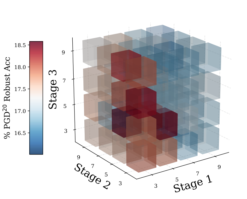
We formulate our goal as searching for an appropriate ratio between total network depth and total network width (in terms of widening factors), i.e., [ $\sum D_{i}:\sum W_{i}$ ], to efficiently allocate computational resources while improving adversarial robustness. Given a target network complexity (e.g., FLOPs budget), we systematically tune the contribution ratio of depth (i.e., $r_{D}=\sum D_{i}/(\sum D_{i}+\sum W_{i})$ ) between $[0.3,0.95)$ and compare the relative changes in robustness under baseline AT. From the results shown in Figure 8, we observe that adversarial robustness improves monotonically as $r_{D}$ increases and peaks at approximately $r_{D}=0.7$ . However, as the $r_{D}$ continues to increase beyond $0.7$ , adversarial robustness starts to deteriorate rapidly. Accordingly, our compound scaling rule, dubbed RobustScaling, is obtained by solving:

\small\begin{split}r_{D}&=\frac{D_{1}+D_{2}+D_{3}}{D_{1}+D_{2}+D_{3}+W_{1}+W_{2}+W_{3}}\\ &=\frac{2D_{3}+2D_{3}+D_{3}}{2D_{3}+2D_{3}+D_{3}+2W_{3}+2.5W_{3}+W_{3}}=0.7\end{split}

such that the $Complexity{\big(\sum D_{i},\sum W_{i}\big)\approx}$ the target. A pictorial illustration of the compound settings under different FLOP budgets is provided in Figure 9(a), along with the standard settings (i.e., WRN-28-10, WRN-70-16, etc.) in Figure 9(b), the settings obtained by independently scaling depth and width in Figures 9(c) and 9(d), respectively. We observe that deep but narrow networks are preferred over wide but shallow networks for adversarial robustness at a given FLOPs budget.

(a) Compound scaling
(

\sum D_{i}:\sum W_{i}=7:3

)

(b) Standard scaling
(i.e., WRN-28-10, WRN-70-16)

D_{1}:D_{2}:D_{3}=2:2:1

)

(d) Scaling by width
(

W_{1}:W_{2}:W_{3}=2:2.5:1

)

Figure 9: Visualization of depth and width distribution among the three stages for (a) our compound scaling, (b) standard scaling, and (c, d) our independent scaling by depth/width. The secondary y-axis shows robust accuracy under baseline adversarial training.

Empirically, we compare our compound scaling to independent scaling by depth/width, the standard scaling (i.e., WRN-28-10, WRN-70-16, etc.), and the existing robust scaling from Huang et al. huang2021exploring under baseline adversarial training in Figure 10. Note that Huang et al. huang2021exploring only report one network, WRN-34-R. But we apply their (width) scaling rule to other WRN networks at different depths and obtain a set of WRN-R networks. We observe that, in general, RobustScaling achieves the best trade-off between robustness and network complexity, yielding networks that offer substantial improvements in robust accuracy over existing scaling methods while being an order of magnitude more efficient. In particular, WRN-A1 (i.e., the least complex network from RobustScaling) is $3.8\times$ more compact (^#Params) and efficient (^#FLOPs) than WRN-34-R huang2021exploring while being similar in adversarial robustness. In addition, WRN-A1 is more adversarially robust than WRN-70-16 (i.e., the most complex network from the standard scaling) while being $14\times$ more compact and $8\times$ more efficient. Our findings suggest that effective compound policies do exist for scaling networks under adversarial training, and our RobustScaling is one such realization.

(a) CW⁴⁰ vs. ^#Params

(b) CW⁴⁰ vs. ^#FLOPs

(d) CW⁴⁰ vs. ^#FLOPs

Figure 10: (a, b) Comparison among standard scaling (blue curve), existing robust scaling huang2021exploring (brown curve), the identified independent depth/width scaling (orange/green curve) from §4.2.1, and the identified compound scaling RobustScaling (red curve) on CIFAR-10. [

D_{1}

D_{2}

D_{3}

] and [

W_{1}

W_{2}

W_{3}

] denote stage-wise depth and width (in terms of widening factors) settings, respectively. For independent depth scaling, we use the width settings from the standard scaling and vice-versa for independent width scaling. All scaling strategies are applied to WRNs (i.e., basic residual block).

Table 2: Comparison of white-box adversarial robustness under baseline AT with TRADES zhang2019theoretically. The best results are in bold, and relative improvements over 2^nd best result in each section are in red. Results are averaged over three runs with different seeds.

Model	^#P (M)	^#F (G)	CIFAR-10				CIFAR-100
Model	^#P (M)	^#F (G)	Clean	PGD²⁰	CW⁴⁰	AutoAttack	Clean	PGD²⁰	CW⁴⁰	AutoAttack
WRN-28-10	36.5	5.20	$84.62_{\pm{0.06}}$	$55.90_{\pm{0.21}}$	$53.15_{\pm{0.33}}$	$51.66_{\pm{0.29}}$	$56.30_{\pm{0.28}}$	$29.91_{\pm{0.40}}$	$26.22_{\pm{0.23}}$	$25.26_{\pm{0.06}}$
RobNet-large-v2	33.3	5.10	$84.57_{\pm{0.16}}$	$52.79_{\pm{0.08}}$	$48.94_{\pm{0.13}}$	$47.48_{\pm{0.04}}$	$55.27_{\pm{0.02}}$	$29.23_{\pm{0.15}}$	$24.63_{\pm{0.11}}$	$23.69_{\pm{0.19}}$
AdvRush ( $7@96$ )	32.6	4.97	$84.95_{\pm{0.12}}$	$56.99_{\pm{0.08}}$	$53.27_{\pm{0.03}}$	$52.90_{\pm{0.11}}$	$56.40_{\pm{0.09}}$	$30.40_{\pm{0.21}}$	$26.16_{\pm{0.03}}$	$25.27_{\pm{0.02}}$
RACL ( $7@104$ )	32.5	4.93	$83.91_{\pm{0.32}}$	$55.98_{\pm{0.15}}$	$53.22_{\pm{0.08}}$	$51.37_{\pm{0.11}}$	$56.09_{\pm{0.08}}$	$30.38_{\pm{0.03}}$	$26.65_{\pm{0.02}}$	$25.65_{\pm{0.10}}$
RobustResNet-A1 (ours)	19.2	5.11	$85.46$ ( $\uparrow\bm{0.5}$ )	$58.74$ ( $\uparrow\bm{1.8}$ )	$55.72$ ( $\uparrow\bm{2.6}$ )	$54.42$ ( $\uparrow\bm{1.5}$ )	$59.34$ ( $\uparrow\bm{2.9}$ )	$32.70$ ( $\uparrow\bm{2.3}$ )	$27.76$ ( $\uparrow\bm{1.1}$ )	$26.75$ ( $\uparrow\bm{1.1}$ )
WRN-34-12	66.5	9.60	$84.93_{\pm{0.24}}$	$56.01_{\pm{0.28}}$	$53.53_{\pm{0.15}}$	$51.97_{\pm{0.09}}$	$56.08_{\pm{0.41}}$	$29.87_{\pm{0.23}}$	$26.51_{\pm{0.11}}$	$25.47_{\pm{0.10}}$
WRN-34-R	68.1	19.1	$85.80_{\pm{0.08}}$	$57.35_{\pm{0.09}}$	$54.77_{\pm{0.10}}$	$53.23_{\pm{0.07}}$	$58.78_{\pm{0.11}}$	$31.17_{\pm{0.08}}$	$27.33_{\pm{0.11}}$	$26.31_{\pm{0.03}}$
RobustResNet-A2 (ours)	39.0	10.8	$85.80$ ( $\uparrow\bm{0.0}$ )	$59.72$ ( $\uparrow\bm{2.4}$ )	$56.74$ ( $\uparrow\bm{2.0}$ )	$55.49$ ( $\uparrow\bm{2.3}$ )	$59.38$ ( $\uparrow\bm{0.6}$ )	$33.0$ ( $\uparrow\bm{1.8}$ )	$28.71$ ( $\uparrow\bm{1.4}$ )	$27.68$ ( $\uparrow\bm{1.4}$ )
WRN-46-14	128	18.6	$85.22_{\pm{0.15}}$	$56.37_{\pm{0.18}}$	$54.19_{\pm{0.11}}$	$52.63_{\pm{0.18}}$	$56.78_{\pm{0.47}}$	$30.03_{\pm{0.07}}$	$27.27_{\pm{0.05}}$	$26.28_{\pm{0.03}}$
RobustResNet-A3 (ours)	75.9	19.9	$86.79$ ( $\uparrow\bm{1.6}$ )	$60.10$ ( $\uparrow\bm{3.7}$ )	$57.29$ ( $\uparrow\bm{3.1}$ )	$55.84$ ( $\uparrow\bm{3.2}$ )	$60.16$ ( $\uparrow\bm{3.4}$ )	$33.59$ ( $\uparrow\bm{3.6}$ )	$29.58$ ( $\uparrow\bm{2.3}$ )	$28.48$ ( $\uparrow\bm{2.2}$ )
WRN-70-16	267	38.8	$85.51_{\pm{0.24}}$	$56.78_{\pm{0.16}}$	$54.52_{\pm{0.16}}$	$52.80_{\pm{0.14}}$	$56.93_{\pm{0.61}}$	$29.76_{\pm{0.17}}$	$27.20_{\pm{0.16}}$	$26.12_{\pm{0.24}}$
RobustResNet-A4 (ours)	147	39.4	$87.10$ ( $\uparrow\bm{1.6}$ )	$60.26$ ( $\uparrow\bm{3.5}$ )	$57.9$ ( $\uparrow\bm{3.4}$ )	$56.29$ ( $\uparrow\bm{3.5}$ )	$61.66$ ( $\uparrow\bm{4.7}$ )	$34.25$ ( $\uparrow\bm{4.5}$ )	$30.04$ ( $\uparrow\bm{2.8}$ )	$29.00$ ( $\uparrow\bm{2.9}$ )

5 Adversarially Robust Residual Networks

We use RobustScaling to scale our RobustResBlock to present a portfolio of adversarially robust residual networks, dubbed RobustResNets, spanning a broad spectrum of model FLOP budgets (i.e., $5$ G - $40$ G FLOPs). For reference, we name them as RobustResNet-A1 to -A4, where the FLOPs budget is doubled for every subsequent network. See Table 7 for detailed specifications. We then compare RobustResNets to a set of representative robust architectures proposed in the literature. These include, RobNet NAS_Meets_Robustness, RACL dong2020adversarially, AdvRush mok2021advrush, and WRN-34-R huang2021exploring. Specifically, we align the network complexity of AdvRush and RACL models by adjusting the number of repetitions of the normal cell $N$ and the input ^#channels of the first normal cell $C$ , denoted as ( $N@C$ ).

Comparison under Baseline Adversarial Training: Table 2 presents the results under baseline adversarial training with TRADES zhang2019theoretically. In general, RobustResNets consistently outperform existing robust networks across multiple datasets, attacks, and model-capacity regions. In particular, RobustResNet-A1 achieves $1.5\%$ higher AutoAttack robust accuracy with $1.7{\times}$ fewer parameters than AdvRush mok2021advrush, a robust block designed by differentiable neural architecture search; RobustResNet-A2 achieves $2.3\%$ higher AutoAttack robust accuracy with $1.8{\times}$ fewer parameters and FLOPs than WRN-34-R huang2021exploring. Additional comparisons under baseline adversarial training methods with different loss functions (i.e., SAT madry2018towards, and MART Wang2020Improving) are presented in Table 3. We observe that the improvements afforded by RobustResNets generalize well to other loss formulations under baseline adversarial training routines.

Table 3: Additional comparison of white-box adversarial robustness under baseline adversarial training with SAT madry2018towards, and MART Wang2020Improving. The best results are in bold, and relative improvements are in red. Results are averaged over three runs with different seeds.

Model	^#P (M)	^#F (G)	SAT madry2018towards		MART Wang2020Improving
Model	^#P (M)	^#F (G)	PGD²⁰	CW⁴⁰	PGD²⁰	CW⁴⁰
WRN-28-10	36.5	5.20	$52.44_{\pm{0.36}}$	$50.97_{\pm{0.09}}$	$57.69_{\pm{0.11}}$	$52.88_{\pm{0.28}}$
RobustResNet-A1	19.2	5.11	$57.62$ ( $\uparrow\bm{5.2}$ )	$56.06$ ( $\uparrow\bm{5.1}$ )	$59.34$ ( $\uparrow\bm{1.7}$ )	$54.42$ ( $\uparrow\bm{1.5}$ )
WRN-34-12	66.5	9.60	$52.85_{\pm{0.40}}$	$51.36_{\pm{0.33}}$	$57.40_{\pm{0.13}}$	$53.11_{\pm{0.00}}$
RobustResNet-A2	39.0	10.8	$58.39$ ( $\uparrow\bm{5.5}$ )	$56.99$ ( $\uparrow\bm{5.6}$ )	$60.33$ ( $\uparrow\bm{2.9}$ )	$55.51$ ( $\uparrow\bm{2.4}$ )
WRN-46-14	128	18.6	$53.67_{\pm{0.03}}$	$52.95_{\pm{0.04}}$	$58.43_{\pm{0.15}}$	$54.32_{\pm{0.17}}$
RobustResNet-A3	75.9	19.9	$58.81$ ( $\uparrow\bm{5.1}$ )	$57.60$ ( $\uparrow\bm{4.7}$ )	$60.95$ ( $\uparrow\bm{2.5}$ )	$56.52$ ( $\uparrow\bm{2.2}$ )
WRN-70-16	267	38.8	$54.12_{\pm{0.08}}$	$50.52_{\pm{0.18}}$	$58.15_{\pm{0.28}}$	$54.37_{\pm{0.07}}$
RobustResNet-A4	147	39.4	$59.01$ ( $\uparrow\bm{4.9}$ )	$57.85$ ( $\uparrow\bm{7.3}$ )	$61.88$ ( $\uparrow\bm{3.7}$ )	$57.55$ ( $\uparrow\bm{3.2}$ )

Comparison under Advanced Adversarial Training: Table 4 presents results under advanced AT with an additional 500K unlabeled external images extracted from the 80M Tiny Images dataset carmon2019unlabeled. RobustResNet-A1 achieves $63.70\%$ AutoAttack robust accuracy with $19.2$ M parameters, ranking 7^th (as of 20th December, 2022) on RobustBench CIFAR-10 leaderboard croce2020robustbench. Note that higher-ranked methods (i.e., top-6 on RobustBench CIFAR-10 leaderboard) use networks WRN-70-16 or WRN-106-16, which have at least $250$ M more parameters than RobustResNet-A1. Furthermore, RobustResNet-A1 is $\sim 1.2\%$ more robust against AutoAttack with $3.5\times$ fewer parameters and $3.7\times$ fewer FLOPs than WRN-34-R huang2021exploring.

Table 4: Comparison of white-box adversarial robustness under advanced adversarial training with extra 500k external data carmon2019unlabeled.

Method	Architecture	^#P (M)	^#F (G)	AutoAttack
RST carmon2019unlabeled	WRN-28-10	$36.5$	$5.20$	$59.53$
AWP wu2020adversarial	WRN-28-10	$36.5$	$5.20$	$60.04$
HAT rade2021reducing	WRN-28-10	$36.5$	$5.20$	$62.50$
Gowal et al. gowal2020uncovering	WRN-28-10	$36.5$	$5.20$	$62.80$
Huang et al. huang2021exploring	WRN-34-R	$68.1$	$19.1$	$62.54$
Ours	RobustResNet-A1	$\bm{19.2}$ ( $\downarrow\bm{3.5\times}$ )	$\bm{5.11}$ ( $\downarrow\bm{3.7\times}$ )	$\bm{63.70}$ ( $\uparrow\bm{1.2}$ )

Table 5 presents results under advanced adversarial training without additional data, either external (e.g., the 500K data carmon2019unlabeled) or generated by generative models (e.g., DDPM gowal2021improving). In particular, RobustResNet-A1 achieves $1.9\%$ higher AutoAttack robust accuracy with $1.9{\times}$ fewer parameters than state-of-the-art¹¹ 1 We consider state-of-the-art without external or generated data. Note that the “Extra data” column of the RobustBench CIFAR-10 leaderboard only accounts for external data; please also see the description under the “Method” column for approaches that do leverage generated data. method built upon WRN-28-10 rebuffi2021data. Furthermore, RobustResNet-A2 is $6.8\times$ more compact (parameters) and $3.7\times$ more efficient (FLOPs) while matching the state-of-the-art AutoAttack robust accuracy. And RobustResNet-A4 achieves $61.10\%$ AutoAttack robust accuracy with $39.4$ M parameters on CIFAR-10 against AutoAttack with $\ell_{\infty}$ perturbations of size $\epsilon=8/255$ —an improvement of $1.0\%$ robust accuracy with $120$ million fewer parameters compared to the state-of-the-art without external or generated data rebuffi2021data.

Table 5: Comparison of white-box adversarial robustness under advanced adversarial training. Our method builds upon Rebuffi et al. rebuffi2021data, which applies CutMix yun2019cutmix data augmentation.

Method	Architecture	^#P (M)	^#F (G)	AutoAttack
TRADES zhang2019theoretically	WRN-34-10	$46.2$	$6.66$	$53.08$
Rebuffi et al. rebuffi2021data	WRN-28-10	$36.5$	$5.20$	$57.50$
Ours	RobustResNet-A1	$\bm{19.2}$ ( $\downarrow\bm{1.9\times}$ )	$\bm{5.11}$ ( $\sim$ )	$\bm{59.39}$ ( $\uparrow\bm{1.9}$ )
Gowal et al. gowal2020uncovering	WRN-70-16	$267$	$\bm{38.8}$	$57.20$
Rebuffi et al. rebuffi2021data	WRN-70-16	$267$	$\bm{38.8}$	$60.07$
Ours	RobustResNet-A2	$\bm{39.0}$ ( $\downarrow\bm{6.8\times}$ )	$\bm{10.6}$ ( $\downarrow\bm{3.7\times}$ )	${60.00}$ ( $\sim$ )
Ours	RobustResNet-A4	${147}$ ( $\downarrow{1.8\times}$ )	$39.4$ ( $\sim$ )	$\bm{61.10}$ ( $\uparrow\bm{1.0}$ )

6 Discussion

This paper identified specific architectural design elements that impact adversarial robustness. The reliability of our observations has been ensured by systematically verifying them on multiple datasets, across multiple adversarial attacks, and over multiple repetitions. We affirm that the proposed RobustResBlock, RobustScaling, and RobustResNet have immediate practical relevance in designing adversarially robust networks. Nonetheless, our observations and contributions have been made through empirical experiments instead of theoretical analysis. However, as is often the case in deep learning (e.g., batch normalization ioffe2015batch, lottery ticket hypothesis frankle2018the, etc.), theoretical analysis usually follows empirical observations. Furthermore, most of the theoretical studies in adversarial robustness have focused on loss formulation. We hope this paper inspires theoretical exploration of the adversarial robustness properties of different architectural design elements as well.

7 Concluding Remarks

Novel architectural designs played a critical role in the overwhelming success of CNNs in various image analysis tasks. Despite this knowledge, studies on adversarial robustness have primarily been limited to a handful of basic residual networks, thus overlooking the impact of architecture on adversarial robustness. However, as we demonstrate in this paper, architectural design significantly affects adversarial robustness. As an illustration, we considered residual networks. We observed through systematically designed experiments that many advancements of residual blocks for standard ERM training translate well to improve adversarial robustness under adversarial training, albeit with minor modifications in some cases.

Based on our observations, we designed RobustResNets as an alternative baseline for standard Wide Residual Networks, the de facto architecture of choice for designing adversarially robust networks. RobustResNets afford significant improvements in adversarial robustness while being more compact than state-of-the-art solutions, both without extra data and with 500K extra data. We hope that RobustResNets can serve as a new benchmark architecture for studying adversarial robustness and that our work inspires future exploration into the adversarial robustness of the wide range of architectures that have already proven effective under standard ERM training.

Acknowledgements

Shihua Huang and Vishnu Naresh Boddeti are supported in part by the following financial assistance award 60NANB18D210 from U.S. Department of Commerce, National Institute of Standards and Technology. Zhichao Lu is supported by the National Natural Science Foundation of China (62106097) and the China Postdoctoral Science Foundation (2021M691424).

References

(1) Jimmy Lei Ba, Jamie Ryan Kiros, and Geoffrey E Hinton. Layer normalization. arXiv preprint arXiv:1607.06450, 2016.
(2) Yutong Bai, Jieru Mei, Alan Yuille, and Cihang Xie. Are transformers more robust than CNNs? In A. Beygelzimer, Y. Dauphin, P. Liang, and J. Wortman Vaughan, editors, Adv. Neural Inform. Process. Syst., 2021.
(3) Nicholas Carlini and David Wagner. Towards evaluating the robustness of neural networks. In IEEE symposium on security and privacy (sp), 2017.
(4) Yair Carmon, Aditi Raghunathan, Ludwig Schmidt, John C Duchi, and Percy S Liang. Unlabeled data improves adversarial robustness. Adv. Neural Inform. Process. Syst., 2019.
(5) George Cazenavette, Calvin Murdock, and Simon Lucey. Architectural adversarial robustness: The case for deep pursuit. In IEEE Conf. Comput. Vis. Pattern Recog., 2021.
(6) Hanlin Chen, Baochang Zhang, Song Xue, Xuan Gong, Hong Liu, Rongrong Ji, and David Doermann. Anti-bandit neural architecture search for model defense. In Eur. Conf. Comput. Vis., 2020.
(7) Tianlong Chen, Zhenyu Zhang, Sijia Liu, Shiyu Chang, and Zhangyang Wang. Robust overfitting may be mitigated by properly learned smoothening. In Int. Conf. Learn. Represent., 2021.
(8) Francesco Croce, Maksym Andriushchenko, Vikash Sehwag, Edoardo Debenedetti, Nicolas Flammarion, Mung Chiang, Prateek Mittal, and Matthias Hein. Robustbench: a standardized adversarial robustness benchmark. arXiv preprint arXiv:2010.09670, 2020.
(9) Francesco Croce and Matthias Hein. Reliable evaluation of adversarial robustness with an ensemble of diverse parameter-free attacks. In Int. Conf. Mach. Learn., 2020.
(10) Sihui Dai, Saeed Mahloujifar, and Prateek Mittal. Parameterizing activation functions for adversarial robustness. In IEEE Security and Privacy Workshops, 2022.
(11) Xiaohan Ding, Xiangyu Zhang, Jungong Han, and Guiguang Ding. Scaling up your kernels to 31x31: Revisiting large kernel design in cnns. In IEEE Conf. Comput. Vis. Pattern Recog., 2022.
(12) Minjing Dong, Yanxi Li, Yunhe Wang, and Chang Xu. Adversarially robust neural architectures. arXiv preprint arXiv:2009.00902, 2020.
(13) Jonathan Frankle and Michael Carbin. The lottery ticket hypothesis: Finding sparse, trainable neural networks. In Int. Conf. Learn. Represent., 2019.
(14) Shang-Hua Gao, Ming-Ming Cheng, Kai Zhao, Xin-Yu Zhang, Ming-Hsuan Yang, and Philip Torr. Res2net: A new multi-scale backbone architecture. IEEE Trans. Pattern Anal. Mach. Intell., 43(2):652–662, 2021.
(15) Ian Goodfellow, Jonathon Shlens, and Christian Szegedy. Explaining and harnessing adversarial examples. In Int. Conf. Learn. Represent., 2015.
(16) Sven Gowal, Chongli Qin, Jonathan Uesato, Timothy Mann, and Pushmeet Kohli. Uncovering the limits of adversarial training against norm-bounded adversarial examples. arXiv preprint arXiv:2010.03593, 2020.
(17) Sven Gowal, Sylvestre-Alvise Rebuffi, Olivia Wiles, Florian Stimberg, Dan Andrei Calian, and Timothy Mann. Improving robustness using generated data. In Adv. Neural Inform. Process. Syst., 2021.
(18) Minghao Guo, Yuzhe Yang, Rui Xu, Ziwei Liu, and Dahua Lin. When nas meets robustness: In search of robust architectures against adversarial attacks. In IEEE Conf. Comput. Vis. Pattern Recog., 2020.
(19) Kaiming He, Xiangyu Zhang, Shaoqing Ren, and Jian Sun. Deep residual learning for image recognition. In IEEE Conf. Comput. Vis. Pattern Recog., 2016.
(20) Kaiming He, Xiangyu Zhang, Shaoqing Ren, and Jian Sun. Identity mappings in deep residual networks. In Eur. Conf. Comput. Vis., 2016.
(21) Andrew Howard, Mark Sandler, Grace Chu, Liang-Chieh Chen, Bo Chen, Mingxing Tan, Weijun Wang, Yukun Zhu, Ruoming Pang, Vijay Vasudevan, et al. Searching for mobilenetv3. In Int. Conf. Comput. Vis., 2019.
(22) Jie Hu, Li Shen, Samuel Albanie, Gang Sun, and Enhua Wu. Squeeze-and-excitation networks. IEEE Trans. Pattern Anal. Mach. Intell., 42(8):2011–2023, 2020.
(23) Hanxun Huang, Yisen Wang, Sarah Erfani, Quanquan Gu, James Bailey, and Xingjun Ma. Exploring architectural ingredients of adversarially robust deep neural networks. Adv. Neural Inform. Process. Syst., 2021.
(24) Shihua Huang, Zhichao Lu, Ran Cheng, and Cheng He. Fapn: Feature-aligned pyramid network for dense image prediction. In Int. Conf. Comput. Vis., 2021.
(25) Sergey Ioffe and Christian Szegedy. Batch normalization: Accelerating deep network training by reducing internal covariate shift. In Int. Conf. Mach. Learn., 2015.
(26) Pavel Izmailov, Dmitrii Podoprikhin, Timur Garipov, Dmitry Vetrov, and Andrew Gordon Wilson. Averaging weights leads to wider optima and better generalization. arXiv preprint arXiv:1803.05407, 2018.
(27) Jia Liu and Yaochu Jin. Multi-objective search of robust neural architectures against multiple types of adversarial attacks. Neurocomputing, 453:73–84, 2021.
(28) Zhuang Liu, Hanzi Mao, Chao-Yuan Wu, Christoph Feichtenhofer, Trevor Darrell, and Saining Xie. A convnet for the 2020s. In IEEE Conf. Comput. Vis. Pattern Recog., 2022.
(29) Aleksander Madry, Aleksandar Makelov, Ludwig Schmidt, Dimitris Tsipras, and Adrian Vladu. Towards deep learning models resistant to adversarial attacks. In Int. Conf. Learn. Represent., 2018.
(30) Jisoo Mok, Byunggook Na, Hyeokjun Choe, and Sungroh Yoon. Advrush: Searching for adversarially robust neural architectures. In Int. Conf. Comput. Vis., 2021.
(31) Xuefei Ning, Junbo Zhao, Wenshuo Li, Tianchen Zhao, Yin Zheng, Huazhong Yang, and Yu Wang. Discovering robust convolutional architecture at targeted capacity: A multi-shot approach. arXiv preprint arXiv:2012.11835, 2020.
(32) Tianyu Pang, Xiao Yang, Yinpeng Dong, Hang Su, and Jun Zhu. Bag of tricks for adversarial training. In Int. Conf. Learn. Represent., 2021.
(33) Chongli Qin, James Martens, Sven Gowal, Dilip Krishnan, Krishnamurthy Dvijotham, Alhussein Fawzi, Soham De, Robert Stanforth, and Pushmeet Kohli. Adversarial robustness through local linearization. Adv. Neural Inform. Process. Syst., 2019.
(34) Rahul Rade and Seyed-Mohsen Moosavi-Dezfooli. Reducing excessive margin to achieve a better accuracy vs. robustness trade-off. In Int. Conf. Learn. Represent., 2021.
(35) Sylvestre-Alvise Rebuffi, Sven Gowal, Dan Andrei Calian, Florian Stimberg, Olivia Wiles, and Timothy Mann. Data augmentation can improve robustness. In Adv. Neural Inform. Process. Syst., 2021.
(36) Leslie Rice, Eric Wong, and Zico Kolter. Overfitting in adversarially robust deep learning. In Int. Conf. Mach. Learn., 2020.
(37) Mark Sandler, Andrew Howard, Menglong Zhu, Andrey Zhmoginov, and Liang-Chieh Chen. Mobilenetv2: Inverted residuals and linear bottlenecks. In IEEE Conf. Comput. Vis. Pattern Recog., 2018.
(38) Vikash Sehwag, Saeed Mahloujifar, Tinashe Handina, Sihui Dai, Chong Xiang, Mung Chiang, and Prateek Mittal. Robust learning meets generative models: Can proxy distributions improve adversarial robustness? In Int. Conf. Learn. Represent., 2022.
(39) Ali Shafahi, Mahyar Najibi, Mohammad Amin Ghiasi, Zheng Xu, John Dickerson, Christoph Studer, Larry S Davis, Gavin Taylor, and Tom Goldstein. Adversarial training for free! Adv. Neural Inform. Process. Syst., 32, 2019.
(40) Vasu Singla, Sahil Singla, Soheil Feizi, and David Jacobs. Low curvature activations reduce overfitting in adversarial training. In Int. Conf. Comput. Vis., 2021.
(41) Christian Szegedy, Wojciech Zaremba, Ilya Sutskever, Joan Bruna, Dumitru Erhan, Ian Goodfellow, and Rob Fergus. Intriguing properties of neural networks. In Int. Conf. Learn. Represent., 2014.
(42) Mingxing Tan and Quoc Le. Efficientnet: Rethinking model scaling for convolutional neural networks. In Int. Conf. Mach. Learn., 2019.
(43) Mingxing Tan and Quoc V Le. Mixconv: Mixed depthwise convolutional kernels. arXiv preprint arXiv:1907.09595, 2019.
(44) Dmitry Ulyanov, Andrea Vedaldi, and Victor Lempitsky. Instance normalization: The missing ingredient for fast stylization. arXiv preprint arXiv:1607.08022, 2016.
(45) Hongjun Wang and Yisen Wang. Self-ensemble adversarial training for improved robustness. In Int. Conf. Learn. Represent., 2022.
(46) Yisen Wang, Xingjun Ma, James Bailey, Jinfeng Yi, Bowen Zhou, and Quanquan Gu. On the convergence and robustness of adversarial training. arXiv preprint arXiv:2112.08304, 2021.
(47) Yisen Wang, Difan Zou, Jinfeng Yi, James Bailey, Xingjun Ma, and Quanquan Gu. Improving adversarial robustness requires revisiting misclassified examples. In Int. Conf. Learn. Represent., 2019.
(48) Yisen Wang, Difan Zou, Jinfeng Yi, James Bailey, Xingjun Ma, and Quanquan Gu. Improving adversarial robustness requires revisiting misclassified examples. In Int. Conf. Learn. Represent., 2020.
(49) Ross Wightman, Hugo Touvron, and Hervé Jégou. Resnet strikes back: An improved training procedure in timm. arXiv preprint arXiv:2110.00476, 2021.
(50) Eric Wong, Leslie Rice, and J Zico Kolter. Fast is better than free: Revisiting adversarial training. arXiv preprint arXiv:2001.03994, 2020.
(51) Dongxian Wu, Shu-Tao Xia, and Yisen Wang. Adversarial weight perturbation helps robust generalization. Adv. Neural Inform. Process. Syst., 2020.
(52) Yuxin Wu and Kaiming He. Group normalization. In Eur. Conf. Comput. Vis., pages 3–19, 2018.
(53) Cihang Xie, Mingxing Tan, Boqing Gong, Alan Yuille, and Quoc V Le. Smooth adversarial training. arXiv preprint arXiv:2006.14536, 2020.
(54) Saining Xie, Ross Girshick, Piotr Dollár, Zhuowen Tu, and Kaiming He. Aggregated residual transformations for deep neural networks. In IEEE Conf. Comput. Vis. Pattern Recog., 2017.
(55) Sangdoo Yun, Dongyoon Han, Seong Joon Oh, Sanghyuk Chun, Junsuk Choe, and Youngjoon Yoo. Cutmix: Regularization strategy to train strong classifiers with localizable features. In Int. Conf. Comput. Vis., 2019.
(56) Sergey Zagoruyko and Nikos Komodakis. Wide residual networks. arXiv preprint arXiv:1605.07146, 2016.
(57) Hongyang Zhang, Yaodong Yu, Jiantao Jiao, Eric Xing, Laurent El Ghaoui, and Michael Jordan. Theoretically principled trade-off between robustness and accuracy. In Int. Conf. Mach. Learn., 2019.
(58) Zhenyu Zhu, Fanghui Liu, Grigorios G Chrysos, and Volkan Cevher. Robustness in deep learning: The good (width), the bad (depth), and the ugly (initialization). arXiv preprint arXiv:2209.07263, 2022.

Appendix A Appendix

A.1 Extended Description of Related Work

Relation to existing works based on NAS. Several recent works sought to find more robust DNN architectures via neural architecture search (NAS) – Guo et al. applied a one-shot NAS algorithm to design the topology of a cell structure (i.e., operations and connections among them) while leaving the network skeleton (i.e., width and depth) to human designs NAS_Meets_Robustness; Mok et al. incorporated the smoothness of a DNN model’s input loss landscape as an additional regularizer for NAS mok2021advrush, among others ning2020discovering; chen2020anti; liu2021multi.

These NAS-based prior arts are limited in the following three aspects: (1) they focus on only one aspect of architecture (i.e., block topology) while leaving other components (e.g., activation, network depth, and width, etc.) to human designs; (2) they treat the design of an adversarially robust architecture as a black-box search problem where minimal architectural insights can be derived; (3) NAS is computationally expensive and adversarial training makes this challenge especially acute.

In contrast, this work presents (i) a holistic study of different aspects of architecture, including block topology, activation, normalization, and scaling factors (i.e., network depth and width); (ii) through controlled and fine-grained experiments, we deliver precise knowledge on the impacts of these choices; (iii) empirically, we demonstrate that the network assembled on top of our derived knowledge outperforms existing networks designed via NAS by at least 2.5% robust accuracy against AutoAttack (see Table 2).

(a) Standard SE

(b) Pre-SE

(d) Conv3

\times

3-SE

(e) Residual SE (ours)

Design

Explanation

(a) Standard SE

Place the SE module posterior to the main components of the residual block as proposed in senet.

(b) Pre-SE

Place the SE module a priori, i.e., before the main components of the residual block, also tried by senet.

Place the SE module in the skip-connection branch, also tried by senet.

(d) Conv3x3-SE

Place the SE module right after the

3\times 3

convolution, as done in MobileNetV3 howard2019searching.

(e) Residual SE (ours)

Add an extra skip connection around the SE module to the standard SE integration design,

similarly to the FSM module from huang2021fapn.

(f)

Design	Reduction ratio	^#P (M)	^#F (G)	Clean Acc. (%)	Robust Acc. (%)
Design	Reduction ratio	^#P (M)	^#F (G)	Clean Acc. (%)	PGD²⁰	CW⁴⁰
w/o SE	–	265	39.0	85.47	57.49	55.07
Standard SE	$r=16$	296	39.1	84.56 (-0.91)	56.87 (-0.62)	54.52 (-0.55)
Conv3 $\times$ 3-SE		273	39.1	85.26 (-0.21)	57.10 (-0.39)	54.77 (-0.40)
Identity-SE		293	39.1	85.20 (-0.27)	57.04 (-0.45)	54.94 (-0.13)
Pre-SE		293	39.1	85.81 (+0.34)	57.31 (-0.18)	55.32 (+0.25)
Residual SE (ours)	$r=16$	296	39.1	85.75 (+0.28)	57.86 (+0.37)	55.95 (+0.88)
	$r=32$	281	39.1	85.22 (-0.25)	57.98 (+0.49)	55.54 (+0.47)
	$r=64$	273	39.1	85.61 (+0.14)	57.77 (+0.28)	56.05 (+0.98)

(g)

(h)

Figure 11: (a) - (e) An overview of SE integration designs studied in this work. (f) Description and (g) ablation results of the SE integration designs are shown in (a) - (e). (h) Comparing residual blocks with and without the proposed residual SE on CIFAR-10 against PGD²⁰ attack.

Relation to other existing works. There are recent works that aim to gain an understanding of adversarial robustness from an architectural perspective xie2020smooth; gowal2020uncovering; cazenavette2021architectural; huang2021exploring; dai2022parameterizing; zhu2022robustness. Among them, huang2021exploring is most closely related to this paper. Accordingly, we provide an elaborated discussion on the relation to huang2021exploring below and refer readers to the Related Work section in §2 for an overview of these methods.

Huang et al. huang2021exploring also investigated the impact of network width and depth via controlled experiments on the adversarial robustness of adversarially trained DNN models. Despite a similar motivation, our work is primarily different and enhanced in the following aspects:

1.

Huang et al. only study network scaling factors (i.e., depth and width), while we study both block topology and network scaling. And as we demonstrated in this paper, both are critical architectural components for improving adversarial robustness. Specifically, we show that (i) improvement on block topology alone leads to $\sim 3\%$ more robust accuracy; (ii) improvement on network scaling alone leads to $\sim 2.5\%$ more robust accuracy; (iii) improvement on both block topology and network scaling leads to $3.5+\%$ more robust accuracy while being $\sim 2\times$ more compact in terms of parameters. All results were evaluated against AutoAttack and relative to WRNs, the de-facto model for studying adversarial robustness.
2.

Huang et al. explored the interplay between network depth and width but observed that the independent scaling rules they identified for depth and width did not work well together and ultimately failed to design a compound rule to scale depth and width simultaneously²² 2 For more details, please refer to Section 4.3 in huang2021exploring.. In contrast, building upon our independent scaling rules, we identify an effective compound rule to simultaneously scale depth and width by properly distributing a given computational budget (e.g., FLOPs) over the number of layers and their width multipliers³³ 3 See Section 4.2.2 for more details.. Empirically, we demonstrate that the compound scaling rule further improves independent scaling of depth and width by $\sim 2\%$ and $\sim 1\%$ more robust accuracy against $CW^{40}$ attack for a small-capacity model, respectively (see Figure 9).
3.

The scaling rule identified by Huang et al. was evaluated at one model capacity only (i.e., $\sim 68$ M ^#Params), while, in this work, we demonstrate the efficacy of our scaling rules (i.e., both independent and compound scaling rules) across a broad spectrum of model-capacities, from $5$ M to $270$ M ^#Params.
4.

Performance-wise, on top of using almost $2\times$ fewer ^#Params and ^#FLOPs, our model (i.e., RobustResNet-A2) consistently exhibits $1.4\%$ - $2.4\%$ higher robust accuracy over the model (i.e., WRN-34-R) scaled by Huang et al. across multiple datasets, attacks, and training settings.

A.2 Extended Description of SE

In this section, we first provide pictorial illustrations and descriptions of the five variations of SE that we tried in Figure 5(a) - 11(e) and Table 11(f), respectively. Then, we provide additional results comparing our proposed residual SE among the five variations of SE in Table 11(g). Our residual SE is a simple yet effective variant of the standard SE that improves adversarial robustness while all other variants fail. Finally, we present the effect of incorporating our residual SE to both basic and bottleneck residual blocks in Figure 11(h).

A.3 Additional Results of Block Topology

In this section, we first provide a visual comparison between post-activation and pre-activation in Figure 12(a), where the standard post-activation he2016deep places the activation function after the weights. In contrast, the pre-activation proposed by he2016identity places the activation function before the weights. Then, we compare the effectiveness of these two arrangements of activation for a non-residual block (i.e., VGG block) on CIFAR-10 in Figure 12(b), followed by comparison over variants of residual blocks with pre-activation on CIFAR-10 against PGD²⁰ attack in Figure 12(c).

(a) Post-activation (top) and Pre-activation (bottom)

(b) Non-residual block

Figure 12: (a) A pictorial illustration of the standard post-activation (Top) and pre-activation arrangements (Bottom). (b) Comparing post- and pre-activation for a non-residual block (i.e., VGG block) on CIFAR-10. (c) Comparison among variants of a residual block with pre-activation on CIFAR-10 against PGD²⁰ attack.

A.4 Additional Results of Aggregated and Hierarchical Convolutions

This section presents pictorial illustrations of aggregated and hierarchical convolutions in Figures 13(a) and 14(a), respectively. Additional results showing the effects of hyperparameters cardinality (for aggregated convolution) and scales (for hierarchical convolution) are presented in Figures 13 (b, c, d) and 14 (b, c, d). Finally, we show the impact of aggregated convolution for the basic block in Figure 15, where we observe that aggregated convolution adversely affects the robustness of the basic block.

(a) Aggregated convolution

(b)

D_{i}=5,W_{i}=12

(c)

D_{i}=7,W_{i}=14

(d)

D_{i}=11,W_{i}=16

Figure 13: (a) Aggregated convolution that splits a regular convolution into multiple parallel convolutions (cardinality). Results are then concatenated. (b, c, d) show the robustness of models from three different capacity regions.

(a) Hierarchical convolution

(b)

D_{i}=5,W_{i}=12

(c)

D_{i}=7,W_{i}=14

(d)

D_{i}=11,W_{i}=16

Figure 14: (a) Hierarchical convolution that splits a regular convolution into multiple hierarchically connected convolutions (scales). Results are then concatenated. (b, c, d) show the robustness of models from three different capacity regions.

(a) PGD²⁰

(b) CW⁴⁰

Figure 15: The impact of aggregated convolution for the basic block. Results show the robustness of the model with

D_{i}=4,W_{i}=10

A.5 Impact of Normalization

This section investigates the relationship between normalization methods and adversarial robustness. In addition to the baseline of Batch Normalization (BN), we consider three other normalization methods, i.e., Group Normalization (GN) wu2018group, and Instance Normalization (IN) ulyanov2016instance. We also confine all blocks in a DNN model to use a single choice of normalization method and repeat the experiment for each technique three times. The experimental results are summarized in Table 6. The baseline normalization method (i.e., BN) outperforms all other alternative normalization methods, particularly on Tiny-ImageNet.

Table 6: The adversarial robustness of the considered normalization methods. We highlight the best results of each section in bold.

	CIFAR-10				CIFAR-100				Tiny-ImageNet			Ave. Rank
	Nat.	PGD²⁰	CW⁴⁰	AA	Nat.	PGD²⁰	CW⁴⁰	AA	Nat.	PGD²⁰	AA	Ave. Rank
BN	85.11	55.36	53.02	51.43	55.77	29.91	26.23	25.35	42.09	20.68	16.25	1.5
GN	85.28	55.82	52.76	51.23	56.60	29.86	26.26	25.09	30.99	16.87	13.01	1.7
IN	85.34	54.49	50.82	49.34	56.56	28.41	24.17	22.68	17.25	10.69	8.18	2.7

(a) CIFAR-10, FGSM

(b) CIFAR-10, PGD²⁰

(d) CIFAR-10, AutoAttack

(e) Tiny-ImageNet, FGSM

(f) Tiny-ImageNet, PGD²⁰

(g) Tiny-ImageNet, CW⁴⁰

(h) Tiny-ImageNet, AutoAttack

Figure 17: The adversarial robustness of different kernel sizes for higher resolution images on CIFAR-10 (Top) and Tiny-ImageNet (Bottom) against FGSM, PGD²⁰, CW⁴⁰, and AutoAttack (from left to right).

Table 7: The specifications of RobustResNets. The stage wise setting is presented using

\begin{bmatrix}{k}\times k\mbox{, \#Ch}\end{bmatrix}

, where

k

denotes the convolution filter size, #Ch denotes the number of output channels, and

\begin{bmatrix}\cdot\end{bmatrix}

indicates our RobustResBlock identified in §4.1.

	Output scale	RobustResNet-A1	RobustResNet-A2	RobustResNet-A3	RobustResNet-A4
Stem	$32\times 32$	3 $\times$ 3, 16, stride 1
Stage 1	$32\times 32$	$\begin{bmatrix}\mbox{1}\times\mbox{1, 160}\\ \mbox{3}\times\mbox{3, 80}\\ \mbox{1}\times\mbox{1, 320}\end{bmatrix}$ $\times$ 14	$\begin{bmatrix}\mbox{1}\times\mbox{1, 224}\\ \mbox{3}\times\mbox{3, 224}\\ \mbox{1}\times\mbox{1, 448}\end{bmatrix}$ $\times$ 17	$\begin{bmatrix}\mbox{1}\times\mbox{1, 256}\\ \mbox{3}\times\mbox{3, 256}\\ \mbox{1}\times\mbox{1, 512}\end{bmatrix}$ $\times$ 22	$\begin{bmatrix}\mbox{1}\times\mbox{1, 320}\\ \mbox{3}\times\mbox{3, 320}\\ \mbox{1}\times\mbox{1, 640}\end{bmatrix}$ $\times$ 27
Stage 2	$16\times 16$	$\begin{bmatrix}\mbox{1}\times\mbox{1, 448}\\ \mbox{3}\times\mbox{3, 448}\\ \mbox{1}\times\mbox{1, 896}\end{bmatrix}$ $\times$ 14	$\begin{bmatrix}\mbox{1}\times\mbox{1, 576}\\ \mbox{3}\times\mbox{3, 576}\\ \mbox{1}\times\mbox{1, 1152}\end{bmatrix}$ $\times$ 17	$\begin{bmatrix}\mbox{1}\times\mbox{1, 704}\\ \mbox{3}\times\mbox{3, 704}\\ \mbox{1}\times\mbox{1, 1408}\end{bmatrix}$ $\times$ 22	$\begin{bmatrix}\mbox{1}\times\mbox{1, 896}\\ \mbox{3}\times\mbox{3, 896}\\ \mbox{1}\times\mbox{1, 1792}\end{bmatrix}$ $\times$ 28
Stage 3	$8\times 8$	$\begin{bmatrix}\mbox{1}\times\mbox{1, 384}\\ \mbox{3}\times\mbox{3, 384}\\ \mbox{1}\times\mbox{1, 768}\end{bmatrix}$ $\times$ 7	$\begin{bmatrix}\mbox{1}\times\mbox{1, 512}\\ \mbox{3}\times\mbox{3, 512}\\ \mbox{1}\times\mbox{1, 1024}\end{bmatrix}$ $\times$ 8	$\begin{bmatrix}\mbox{1}\times\mbox{1, 640}\\ \mbox{3}\times\mbox{3, 640}\\ \mbox{1}\times\mbox{1, 1280}\end{bmatrix}$ $\times$ 11	$\begin{bmatrix}\mbox{1}\times\mbox{1, 768}\\ \mbox{3}\times\mbox{3, 768}\\ \mbox{1}\times\mbox{1, 1536}\end{bmatrix}$ $\times$ 13
Tail	$1\times 1$	Global average pool

A.6 Impact of Convolution Kernel Size

Larger kernel sizes have been shown to be beneficial on standard problems tan2019mixconv; liu2022convnet; ding2022scaling under standard ERM training. We evaluate large kernel sizes for adversarial robustness. Specifically, we allow the kernel size $K_{i\in\{1,2,3\}}$ for each stage to be among {3 $\times$ 3, 5 $\times$ 5, 7 $\times$ 7, 9 $\times$ 9} while using the default options for all other settings as described in §3. We evaluate all the $4^{3}=64$ possible networks with all possible settings for the kernel size. Figure 16 shows our results. We observe that, in general, a larger kernel size does not necessarily lead to better adversarial robustness. We repeat the experiment at higher image resolutions to verify if this observation is specific to low-resolution images. Specifically, we upsample the images to the following sizes: { $64\times 64$ , $96\times 96$ , $128\times 128$ }. We constrain all stages to use a canonical kernel size and use a stride of two in the first block of the first stage when the image resolution is higher than $64\times 64$ . Figure 17 presents these results. Empirically, we observe that larger kernels start to improve adversarial robustness noticeably when the image size increases to $128\times 128$ , particularly on Tiny-ImageNet. However, adversarial robustness on upsampled images is consistently worse than that of smaller images. Thus, we argue that a kernel size of $3\times 3$ remains the preferred choice for adversarial robustness.

A.7 Extended discussion of RobustResNets

In this section, we provide detailed specifications of RobustResNetA1 - A4 in Table 7.

Revisiting Residual Networks for Adversarial Robustness: An Architectural Perspective