SeqDiffuSeq: Text Diffusion with Encoder-Decoder Transformers
Abstract
The diffusion model, a new generative modeling paradigm, has achieved great success in image, audio, and video generation. However, considering the discrete categorical nature of the text, it is not trivial to extend continuous diffusion models to natural language. In this work, we propose SeqDiffuSeq, a text diffusion model, to approach sequence-to-sequence text generation with an encoder-decoder Transformer architecture. To improve the generation performance, SeqDiffuSeq is equipped with the self-conditioning technique and our newly proposed adaptive noise schedule technique. Self-conditioning enables SeqDiffuSeq to better use the predicted sequence information during the generation process. The adaptive noise schedule balances the difficulty of denoising across time steps at the token level. Experiment results illustrate the improved performance on five sequence-to-sequence generation tasks compared to other diffusion-based models regarding text quality and inference time. We have released our codes. 11 1 https://github.com/Yuanhy1997/SeqDiffuSeq
1 Introduction
Generative modeling is drawing more attention in recent years of machine learning research due to the development of diffusion models (Ho et al. 2020). Diffusion models define the forward process and the reverse process where the former gradually diffuses data to random noise while the latter recovers data from random noise iteratively, which have shown superior performance on synthesizing images (Rombach et al. 2021), audios (Kong et al. 2020), and videos (Ho et al. 2022) over other generative methods, such as generative adversarial network (GAN) (Goodfellow et al. 2014) and normalizing flow (Kobyzev et al. 2021).
It is not trivial to extend diffusion models to the generation of natural languages. Most of the existing diffusion models are applied to continuous feature space (Ho et al. 2020; Nichol and Dhariwal 2021) while texts are sequences of discrete categorical tokens. Recently, research has explored categorical diffusion models in discrete space for text generation (Hoogeboom et al. 2021; Austin et al. 2022). There also exists research such as DiffusionLM (Li et al. 2022) that applies continuous diffusion models to word embedding. However, these works only focus on unconditional and controlled text generation.
Sequence-to-sequence text generation is a fundamental natural language processing setting and covers various practical downstream tasks, such as dialogue (Ni et al. 2021) and machine translation (Liu et al. 2020). In recent practice, researchers resort to auto-regressive (AR) (Dai et al. 2019) or non-auto-regressive (NAR) (Gu et al. 2019) Transformers for the tasks, and achieve good generation performance. Using diffusion models, a recent work named DiffuSeq (Gong et al. 2022) applies the diffusion-based method for sequence-to-sequence text generation. They deploy encoder-only Transformers and partially define diffusion and denoising processes on output sequences.
In this work, we explore diffusion models with encoder-decoder Transformer architecture for sequence-to-sequence generation. We propose SeqDiffuSeq which extends the continuous diffusion framework proposed in DiffusionLM (Li et al. 2022) to sequence-to-sequence settings. We equip SeqDiffuSeq with the self-conditioning technique (Chen et al. 2022) and our newly proposed adaptive noise schedule. Self-conditioning helps the model better capture the information from former iterations during the generation. The proposed adaptive noise schedule learns a token-level noise schedule to better control the amount of noise injected and information recovered during the forward and reverse process (Nichol and Dhariwal 2021).
We conduct experiments on five generation tasks. Results show that SeqDiffuSeq achieves competitive performance compared with AR and NAR baselines in terms of generation quality and diversity. SeqDiffuSeq also shows improved generation performance and inference speed compared to text diffison model DiffuSeq. Ablation studies demonstrate that our model can benefit from self-conditioning and adaptive noise schedule techniques, and both are complementary to each other in sequence-to-sequence settings.
To summarize, the main contributions of this work are as follows:
- 1.
We propose SeqDiffuSeq that extends the continuous text diffusion model to sequence-to-sequence text generation with encoder-decoder Transformer architecture.
- 2.
The self-conditioning and newly proposed adaptive noise schedule technique can effectively improve the generation quality of the text diffusion model.
- 3.
Experiments show SeqDiffuSeq achieves promising performance with the previous diffusion-based method DiffuSeq as well as AR and NAR models on five generation tasks.
2 Related Work
Since the great success of diffusion models in vision (Ho et al. 2020; Rombach et al. 2021; Song et al. 2021), researchers have explored extending diffusion models to text generation. Considering the discrete and categorical nature of texts, Multinomial Diffusion (Hoogeboom et al. 2021) and D3PM (Austin et al. 2021) are proposed for modeling categorical data. They define discrete diffusion models using discrete categorical transitions directly on texts. DiffusionBERT (He et al. 2022) follows D3PM and introduces pre-trained models for language modeling. Besides, recent research also explores converting texts into continuous features to adapt to diffusion models. Bit Diffusion (Chen et al. 2022) encodes discrete data as binary bits and treats these binary bits as real number features. Yu et al. 2022 is proposed to build text diffusion models in continuous latent space. DiffusionLM (Li et al. 2022) uses the word embedding space for continuous diffusion models and introduces auxiliary losses to enable joint learning of embedding and network parameters. Following DiffusionLM, recent research explores improving text generation quality (Strudel et al. 2022), and DiffuSeq (Gong et al. 2022) extends it to sequence-to-sequence settings. Compared to DiffuSeq, we propose a different model architecture and self-conditioning and adaptive noise schedule techniques to improve sequence-to-sequence generation performance.
Noise schedules in diffusion models control the level of noise injected and the level of information recovered in the forward and reverse process respectively. Previous research in vision and texts demonstrates that appropriate noise schedule design can improve the generation quality performance of diffusion models (Nichol and Dhariwal 2021; Li et al. 2022). Concurrently, DiffusionBERT (He et al. 2022) proposes a spindle schedule for language modeling, and CDCD (Dieleman et al. 2022) designs a learned noise schedule for language modeling and machine translation. Different from both concurrent works, SeqDiffuSeq is proposed with a token-level noise schedule that balances the difficulty of denoising across time steps. Gao et al. 2023 proposes Difformer and is orthogonal to our work.
3 Preliminary
Diffusion model is generally formulated by a designed forward diffusion process and a learnt reverse denoising process. In the forward diffusion process, samples gradually mix with random noise, while in the reverse denoising process, the random noise is gradually denoised to generate synthetic samples. In this work, our diffusion model adopts the forward and reverse processes proposed in DDPM (Ho et al. 2020).
For the forward process, given a sample from a real-world data distribution . At each time step , a noise sample is sampled from , where control the noise added at time step . In this regard, when is large enough, a real-world sample will gradually and ultimately diffuse to a standard Gaussian noise distribution.
For the reverse process, the diffusion model uses a learnt parameterized denoising distribution to gradually recover samples from noise. The denoising distribution is parameterized by and is to fit the posterior distribution of the forward process. can be derived as:
| (1) |
In this equation,
| (2) | |||
| (3) |
With learnt denoising distribution , a synthetic real-world sample can be generated from pure random noise step-by-step.

4 Approach
In this section, we present the main design of our proposed SeqDiffuSeq for sequence-to-sequence language generation. The overview of SeqDiffuSeq is depicted in Figure 1. In the following sections, the input and output sequences are denoted as and respectively. For the -th token in , the token is denoted as , where and represents the maximum output sequence word length. In order to avoid lengthy notations, we omit the indices referring to different data samples.
4.1 Diffusion Model
Forward Process
To fit diffusion models to sequence-to-sequence settings, we extend the text diffusion model, DiffusionLM (Li et al. 2022).
In the sequence-to-sequence setting, the forward process gradually changes the target output sequence to random noise. Diffusing to pure random noise is independent of the input sequence . For the sequence , we use an embedding function to map the word tokens to continuous word embedding , where represents the dimension of embedding and represents the parameters of the word embedding function. The embedding for the sequence is defined by stacking the tokens’ embedding and is denoted as . At the beginning of the forward process, a Markovian transition parameterized by is added. Extended by , the forward process can continue to diffuse continuous features of iteratively. For each time step , we apply the diffusion distribution to get noisier samples. Ultimately, the output sequence becomes which is nearly pure random noise following standard Gaussian distribution.
Reverse Process
Diffusion models generate the synthetic samples by successively sampling the denoising distribution in the reverse process. For each time step in the reverse process, a learnt denoising distribution parameterized by generates samples conditioned on the former noisier samples . In the sequence-to-sequence setting, the generated sequences correlate to input sequences. Therefore, the denoising distribution is additionally conditioned on the input sequence , and . After the reverse denoising process reaches , we round each column of the generated to its nearest word in the embedding space by the rounding distribution to generate the final word sequences.
Training Objective
We optimize and embedding parameters by minimizing the variational bound of the data log-likelihood:
| (4) |
The training objective is to narrow down the discrepancy between and the posterior in the forward process. Since follows the form of Gaussian distribution, we parameterize the denoising distribution following Gaussian distribution family and where
| (5) |
is named the denoising function and predicts the estimated output embedding sequences at each reverse step . Then according to density functions and following Gaussian distribution, the objective can be further simplified as:
| (6) |
where for efficient sampling of during training, and . We leave the detailed derivation to Appendix D. The training objective becomes to fit and the denoising function , which we can model with encoder-decoder Transformers architectures. During training, the sampling distribution contains trainable parameters of word embedding. We can backpropagate through this with reparameterization trick (Kingma and Welling 2013).
Denoising with Encoder-Decoder Framework
Unlike DiffuSeq (Gong et al. 2022) using encoder-only Transformer architecture, we propose using an encoder-decoder Transformers architecture to model the input and output text sequences. For , we use the encoder to process the input sequences and use the decoder to model the noisy output sequence . Following the previous work (Li et al. 2022), we inject time step information by adding time step embedding to . Using the encoder-decoder architecture has computational convenience during generation because the input sequences only require one forward computation through the encoder network during the whole reverse process. Considering the reverse process requires thousands of iterations to generate the output sequences of high quality, the saving of computational resources can be significant.
During training and generation, the function generates denoised samples at the sequence level. Therefore making predictions from the denoising function resembles the non-autoregressive natural language generation. In this regard, we use a decoder with full attention matrices instead of causal attention matrices to model at the sequence level.
4.2 Self-Conditioning
At each time step in the reverse process, the denoising function makes output sequence predictions based on the noisier sample . is sampled from the former denoising distribution by mixing former sequence prediction , and random noise. In this regard, part of the information contained in the former prediction is discarded. Bit-Diffusion (Chen et al. 2022) proposed the self-conditioning technique mitigating this waste of information by additionally taking former sequence predictions as inputs. The denoising function is formulated as . Self-conditioning may enable the denoising function to refine the former sequence predictions rather than make new predictions from scratch. It is empirically verified that the self-conditioning technique can boost the performance of text diffusion models (Strudel et al. 2022).
To fit the technique into the Transformers modeling of in our sequence-to-sequence setting, the sequence features from the former predictions are concatenated with noisier sequence features on the embedding dimension. Hence, the dimension of input features of Transformer decoder becomes . Since the former sequences at time step are sampled successively from to which is computational-tedious during training, we take an efficient training scheme. With half probability, is trained by setting the input to . Otherwise, is first estimated by and then is used for self-conditioning training. Under the second circumstance, we do not backpropagate through the first forward propagate estimated .
4.3 Adaptive Noise Schedule
In the domain of vision and audio, the generated sample quality (Nichol and Dhariwal 2021) and likelihood estimation (Kingma et al. 2021) may potentially benefit from different appropriate time schedules. Previous research uses different simple functions such as linear function (Ho et al. 2020) or cosine function (Nichol and Dhariwal 2021) of against time step to design noise schedules. Such designs may results in unbalanced denoising difficulties for each step and lead to unsatisfying generation quality. Some works proposed to alleviate this problem by importance sampling (Li et al. 2022) or loss reweighing (Gong et al. 2022).
We propose a novel adaptive noise schedule at the token-level. Firstly, we propose to adaptively adjust the time schedules during training to make the denoising difficulties of predicting output sequence increase linearly with respect to the time step. Secondly, we separately set adaptive noise schedule for different token positions, unlike previous text diffusion research that only designs noise schedules on the whole sequence level. Since the intrinsic features for embedding sequences are different across token positions within, we assume that for different token positions the expected noise schedules are different.
Concretely, we measure the difficulties of denoising task at each time step and token position by the training losses . We use the schedule of which ranges from 0 to 1 to access the noise schedule design. controls the noise level at each time step . Our adaptive noise schedule for each token position is to fit a mapping between and by linear interpolation. For time step , ,
| (7) |
After initializing a noise schedule, we record the loss 22 2 We do not record the losses for the padding tokens.. The mapping is fitted after each training period. Ideally, the training losses should be monotonic with respect to the time step since for larger the input features to the denoising function are noisier. However, overall time step is usually by thousands, hence this results in a fine-grained discretization of . Due to the empirical loss estimation errors, training losses may not be monotonic between some successive time steps. To alleviate this issue and fit a smoother mapping , we form a coarse-grained discretization for and : , , , where is the stride to evenly downsample and rounds the number down to it nearest integer.
With the learnt linear interpolation mapping , we can obtain the adjusted discretized noise schedule by where ’s are evenly taken between the minimum and maximum recorded values. As the training progresses, we adaptively calibrate the noise schedule by repeating the above-mentioned procedure once per training updates. The pseudo-code for setting adaptive noise schedules during training is shown in Algorithm 1.
5 Experiments
5.1 Datasets
We conduct experiments on six datasets across five different text generation tasks: Quora Question Pairs (QQP) (DataCanary et al. 2017) for Paraphrase Generation, Wiki-Auto (Jiang et al. 2020) for Text Simplification, Quasar-T (Dhingra et al. 2017) for Question Generation, Commonsense Conversation Dataset (CCD) (Zhou et al. 2018) for Dialogue Generation as well as the German(DE)-English(EN) pairs of IWSLT14 and WMT14 for Machine Translation. Detailed introductions and statistics of the datasets as shown in Appendix E.
| QQP | Wiki-Auto | |||||
| BLEU | BERTScore | dist. 1 | BLEU | BERTScore | dist. 1 | |
| Transformers | 5.80 | 53.92 | 78.89 | 24.45 | 75.90 | 88.86 |
| GPT2-large FT | 20.59 | 83.63 | 98.19 | 26.93 | 78.82 | 94.64 |
| LevT | 22.68 | 83.44 | 97.90 | 20.52 | 72.54 | 97.15 |
| DiffuSeq | 18.47 | 79.47 | 97.61 | 29.89 | 79.12 | 92.33 |
| DiffuSeq w/ MBR=10 | 24.13 | 83.65 | 98.07 | 36.43 | 81.39 | 92.61 |
| SeqDiffuSeq | 23.28 | 82.91 | 98.06 | 37.09 | 82.11 | 90.81 |
| SeqDiffuSeq w/ MBR=10 | 24.34 | 84.00 | 98.07 | 37.12 | 82.14 | 90.77 |
| Quasar-T | CCD | |||||
| BLEU | BERTScore | dist. 1 | BLEU | BERTScore | dist. 1 | |
| Transformers | 3.64 | 53.34 | 82.36 | 1.89 | 47.81 | 74.93 |
| GPT2-large FT | 11.10 | 63.46 | 96.70 | 1.25 | 52.93 | 92.44 |
| LevT | 9.30 | 54.91 | 89.14 | 1.58 | 47.60 | 97.26 |
| DiffuSeq | 15.84 | 59.39 | 91.12 | - | - | - |
| DiffuSeq w/ MBR=10 | 17.01 | 60.95 | 90.72 | 1.39 | 51.31 | 94.67 |
| SeqDiffuSeq | 17.20 | 61.35 | 92.70 | 0.84 | 43.82 | 96.50 |
| SeqDiffuSeq w/ MBR=10 | 17.46 | 61.74 | 92.48 | 1.12 | 44.25 | 96.08 |
| IWSLT14 | WMT14 | |||||
| EN-DE | DE-EN | EN-DE | DE-EN | |||
| SacreBLEU | SacreBLEU | SacreBLEU | BLEU | SacreBLEU | BLEU | |
| Transformers | 26.51 | 33.81 | 26.20 | 27.48 | 30.20 | 31.19 |
| CMLM w/ iter=1 | 14.36 | 21.46 | - | 18.05 | - | 21.83 |
| CMLM w/ iter=4 | 23.74 | 32.83 | - | 25.94 | - | 29.90 |
| CDCD | - | - | 19.30 | - | 24.90 | - |
| CDCD w/ MBR=10 | - | - | 19.70 | - | 25.40 | - |
| SeqDiffuSeq | 21.96 | 30.16 | 19.16 | 23.63 | 23.28 | 25.22 |
| SeqDiffuSeq w/ MBR=10 | 22.12 | 30.45 | 19.76 | 24.24 | 23.93 | 25.90 |
5.2 Baselines
We consider three kinds of models as baselines. First, vanilla encoder-decoder Transformers and pre-trained GPT-2 are selected as strong AR baselines. Second, since SeqDiffuSeq denoises outputs at the sequence level, we compare it with an NAR baseline Levenshtein Transformer (LevT) (Gu et al. 2019). For machine translation, we also use CMLM (Ghazvininejad et al. 2019) which is an NAR translation method with iterative refinement as baselines. Besides, we compare it to other diffusion-based methods. DiffuSeq (Gong et al. 2022) is a recently proposed text diffusion model using an encoder-only Transformer structure. We also compare with concurrently proposed CDCD (Dieleman et al. 2022) on machine translation.
5.3 Implementation Details
We use a 6 layers encoder-decoder Transformer (Vaswani et al. 2017) with GeLU activation (Hendrycks and Gimpel 2016). For the diffusion process, we set the maximum diffusion step to 2000, and use the sqrt schedule from DiffusionLM (Li et al. 2022) to initialize the adaptive time schedule. For translation tasks, we construct vocabulary using BPE (Sennrich et al. 2016). The vocabulary size is set to 10,000 for IWSLT14 and 32,768 for WMT14. For other tasks, we use the vocabulary of bert-base-uncased (Devlin et al. 2019).
For training of SeqDiffuSeq, we use a learning rate of with 10,000 warm-up steps and a linearly-decreasing schedule. The proposed adaptive noise schedule is updated every 20,000 training steps and is set to 20. We explore maximum Bayes risk (MBR) decoding (Koehn 2004) following previous research (Li et al. 2022) for improving generation quality during inference. Details on experiment settings and MBR are in Appendix F.
| IWSLT14 | Paraphrase | Text Simplification | ||||||
|---|---|---|---|---|---|---|---|---|
| EN-DE | DE-EN | QQP | Wiki-Auto | Avg. BLEU | ||||
| S-BLEU | S-BLEU | BLEU | BERTSco. | BLEU | BERTSco. | |||
| SeqDiffuSeq | 21.96 | 30.16 | 23.28 | 83.91 | 37.09 | 82.11 | - | |
| w/o Apt. Sche. | 19.89 | 28.60 | 21.82 | 81.78 | 33.04 | 79.74 | -2.29 | |
| w/o Self-Cond. | 20.76 | 28.28 | 21.64 | 81.45 | 36.46 | 81.62 | -1.34 | |
| w/o Apt. Sche. | 17.50 | 24.39 | 19.73 | 79.95 | 28.03 | 76.06 | -5.71 | |

5.4 Main Results
To assess the generation quality of each model, we use BLEU (Papineni et al. 2002) and BERTScore (Zhang et al. 2020) as metrics. We also use distinct uni-gram (dist.1) to measure the word diversity within generated sentences. A high dist.1 score indicates fewer repeated words. For machine translation tasks, we additionally consider SacreBLEU (Post 2018). The results are listed in Table 1. To better present the generation performance, we provide human evaluation results in Appendix I.
Primarily, for text generation quality, our proposed SeqDiffuSeq achieves much better performance measured by BLEU than DiffuSeq and other baselines with single generation on QQP, Wiki-Auto, and Quasar-T. On Wiki-Auto and Quasar-T, SeqDiffuSeq even achieves better performance with single generation than recently proposed DiffuSeq with MBR of 10 candidates. When incorporating with MBR, SeqDiffuSeq enjoys a boost of performance and achieves superior results over all baselines on QQP, Wiki-Auto, and Quasar-T. The performance is better than the pre-trained then fine-tuned GPT-2 with more parameters on Wiki-Auto and QQP. This indicates that SeqDiffuSeq can generate texts with good quality for sequence-to-sequence tasks (except CCD that all models have inferior performance). On translation tasks, the performance lags behind the AR Transformers baseline consistently across different datasets, while compared with NAR methods, SeqDiffuSeq consistently surpasses CMLM with 1 refinement iteration by 6.32 and 6.75 averaged points across four datasets without and with MBR. CMLM with 4 iterations has better performance. When comparing with CDCD, the performance with and without MBR are competitive on WMT14 EN-DE while the performance is worse on DE-EN. For diversity within sequences, texts generated by SeqDiffuSeq have fewer repeated words averagely than Transformers and DiffuSeq.
The largest improvement over MBR inference with 10 candidates is 1.06 BLEU score on QQP. The amount of this marginal improvement is consistent with concurrently proposed CDCD on WMT14. We will give more in-depth analyses of MBR in the following sections.
6 Analysis and Discussion
6.1 Ablation Study
To verify the effectiveness of the proposed techniques in SeqDiffuSeq, we conduct ablation studies on QQP, Wiki-Auto, and IWSLT14. As shown in Table 2, after removing the adaptive noise schedule from SeqDiffuSeq and instead using the fixed sqrt schedule proposed in DiffusionLM (), the performance drops consistently and the BLEU scores decrease by 2.29 on average. Without self-conditioning (), the performance also degrades by 1.34 on average. By further removing adaptive noise schedule (), the performance drops sharply by 5.71 on average and the largest drop in terms of BLEU is 8.43 on Wiki-Auto. Comparing adaptive noise schedule and self-conditioning technique, it is illustrated that our proposed adaptive noise schedule brings larger improvement and two techniques are complementary to each other.
6.2 Time Schedule
It is verified in the ablation study that the proposed adaptive noise schedule can improve sequence-to-sequence text generation. On the IWSLT14 DE-EN dataset, we visualize the adaptive noise schedules as well as the loss at each time step with and without adaptive noise schedule. For the adaptive noise schedule, we plot at different token positions against the diffusion time step . And for losses, we plot averaged training losses at each position against time step . Depicted in Figure 2, the dashed line in the first sub-figure shows the sqrt schedule, while the other lines represent the noise schedules at different token positions. The figure shows that the adaptive noise schedules deviate from the sqrt schedule. At both ends of time steps, the adaptive noise schedules are flatter compared to sqrt schedule, especially for tokens at larger position orders. Besides, adaptive noise schedules are diverse for different positions, although the trends along time steps are similar. For the token positions at larger orders, the noise schedule lines move toward the lower-left direction. Therefore, at each time step, the tokens at earlier positions have smaller noise than later positions. The information of tokens on the left is recovered earlier at each step. SeqDiffuSeq resembles the left-to-right generation of texts. Through a case study in Appendix J, the phenomenon is also verified.
| Time | Accelerate | |
|---|---|---|
| DiffuSeq | 317 sec. | - |
| SeqDiffuSeq | 89 sec. | 3.56 |
Comparing the second and third sub-figures, the losses with adaptive noise schedule increase linearly with respect to time steps as expected. At each time step, the losses at earlier token positions are smaller, indicating earlier tokens are easier to generate for SeqDiffuSeq . More visualizations on other datasets are listed in Appendix H.

6.3 Inference Speed
We compare SeqDiffuSeq with DiffuSeq in terms of inference time in Table 3. Our SeqDiffuSeq achieves 3.56 times acceleration generating one batch of text samples. The acceleration mainly originated from: (1) SeqDiffuSeq only requires forward computation of encoder once, while DiffuSeq needs to run forward computation for the input sequences for each diffusion step; (2) At each time step, SeqDiffuSeq only models the output sequence, while DiffuSeq has to model the concatenation of both input and output sequences.
6.4 MBR Inference
It is shown in Table 1 that MBR with 10 candidates improves DiffuSeq to more than 6 BLEU score, while improves SeqDiffuSeq by 1.06 BLEU score on QQP. In Figure 3, we plot SacreBLEU scores and Diverse 4-gram (Div.4) scores (Deshpande et al. 2018) against MBR candidate numbers. Div.4 measures the proportion of distinct 4-grams in a set of generated sequences. A higher Div.4 score means better sequence-level diversity by different generation runs. The figure shows that the self-conditioning technique and adaptive noise schedule make the text diffusion model generate less diverse sequences, and the single generated sequence will have higher quality with both techniques. Self-conditioning technique and adaptive noise schedule deliver a trade-off between generation quality and generation diversity. With both techniques, MBR inference is needless to generate high-quality samples for SeqDiffuSeq resulting in a more efficient generation procedure. We also propose a new sampling scheme to compensate the marginal MBR improvements for SeqDiffuSeq which is discussed in detail in Appendix G.
7 Conclusion
In this work, we explore to approach sequence-to-sequence text generation with continuous diffusion models. We propose SeqDiffuSeq which uses an encoder-decoder Transformers architecture to learn the denoising function. In order to improve text generation performance, the denoising function in SeqDiffuSeq is integrated with self-conditioning technique. SeqDiffuSeq also includes a newly proposed adaptive noise schedule which makes the denoising difficulty evenly distributed across all time steps and assigns exclusive noise schedules for tokens from different positional orders. Through experiments, we illustrate the superior performance of SeqDiffuSeq in terms of generation quality and inference speed and provide insights into our proposed adaptive noise schedule technique.
References
- Ho et al. (2020) Ho, J.; Jain, A.; Abbeel, P. Denoising diffusion probabilistic models. Advances in Neural Information Processing Systems 2020, 33, 6840–6851.
- Rombach et al. (2021) Rombach, R.; Blattmann, A.; Lorenz, D.; Esser, P.; Ommer, B. High-Resolution Image Synthesis with Latent Diffusion Models. 2021; pp 10674–10685.
- Kong et al. (2020) Kong, Z.; Ping, W.; Huang, J.; Zhao, K.; Catanzaro, B. Diffwave: A versatile diffusion model for audio synthesis. arXiv preprint arXiv:2009.09761 2020,
- Ho et al. (2022) Ho, J.; Salimans, T.; Gritsenko, A.; Chan, W.; Norouzi, M.; Fleet, D. J. Video Diffusion Models. ArXiv 2022, abs/2204.03458.
- Goodfellow et al. (2014) Goodfellow, I.; Pouget-Abadie, J.; Mirza, M.; Xu, B.; Warde-Farley, D.; Ozair, S.; Courville, A.; Bengio, Y. Generative Adversarial Nets. Advances in Neural Information Processing Systems. 2014.
- Kobyzev et al. (2021) Kobyzev, I.; Prince, S. J.; Brubaker, M. A. Normalizing Flows: An Introduction and Review of Current Methods. IEEE Transactions on Pattern Analysis and Machine Intelligence 2021, 43, 3964–3979.
- Nichol and Dhariwal (2021) Nichol, A. Q.; Dhariwal, P. Improved Denoising Diffusion Probabilistic Models. 2021; https://openreview.net/forum?id=-NEXDKk8gZ.
- Hoogeboom et al. (2021) Hoogeboom, E.; Nielsen, D.; Jaini, P.; Forré, P.; Welling, M. Argmax Flows and Multinomial Diffusion: Learning Categorical Distributions. Advances in Neural Information Processing Systems. 2021; pp 12454–12465.
- Austin et al. (2022) Austin, E.; Zaïane, O. R.; Largeron, C. Community Topic: Topic Model Inference by Consecutive Word Community Discovery. Proceedings of the 29th International Conference on Computational Linguistics. Gyeongju, Republic of Korea, 2022; pp 971–983.
- Li et al. (2022) Li, X. L.; Thickstun, J.; Gulrajani, I.; Liang, P.; Hashimoto, T. B. Diffusion-LM Improves Controllable Text Generation. Advances in Neural Information Processing Systems 2022,
- Ni et al. (2021) Ni, J.; Young, T.; Pandelea, V.; Xue, F.; Adiga, V. V.; Cambria, E. Recent Advances in Deep Learning Based Dialogue Systems: A Systematic Survey. ArXiv 2021, abs/2105.04387.
- Liu et al. (2020) Liu, Y.; Gu, J.; Goyal, N.; Li, X.; Edunov, S.; Ghazvininejad, M.; Lewis, M.; Zettlemoyer, L. Multilingual Denoising Pre-training for Neural Machine Translation. Transactions of the Association for Computational Linguistics 2020, 8, 726–742.
- Dai et al. (2019) Dai, Z.; Yang, Z.; Yang, Y.; Carbonell, J.; Le, Q.; Salakhutdinov, R. Transformer-XL: Attentive Language Models beyond a Fixed-Length Context. Proceedings of the 57th Annual Meeting of the Association for Computational Linguistics. Florence, Italy, 2019; pp 2978–2988.
- Gu et al. (2019) Gu, J.; Wang, C.; Zhao, J. Levenshtein Transformer. Neural Information Processing Systems. 2019.
- Gong et al. (2022) Gong, S.; Li, M.; Feng, J.; Wu, Z.; Kong, L. Diffuseq: Sequence to sequence text generation with diffusion models. arXiv preprint arXiv:2210.08933 2022,
- Chen et al. (2022) Chen, T.; Zhang, R.; Hinton, G. Analog Bits: Generating Discrete Data using Diffusion Models with Self-Conditioning. 2022; https://arxiv.org/abs/2208.04202.
- Song et al. (2021) Song, Y.; Sohl-Dickstein, J.; Kingma, D. P.; Kumar, A.; Ermon, S.; Poole, B. Score-Based Generative Modeling through Stochastic Differential Equations. International Conference on Learning Representations. 2021.
- Austin et al. (2021) Austin, J.; Johnson, D. D.; Ho, J.; Tarlow, D.; van den Berg, R. Structured denoising diffusion models in discrete state-spaces. Advances in Neural Information Processing Systems 2021, 34, 17981–17993.
- He et al. (2022) He, Z.; Sun, T.; Wang, K.; Huang, X.; Qiu, X. DiffusionBERT: Improving Generative Masked Language Models with Diffusion Models. arXiv preprint arXiv:2211.15029 2022,
- Yu et al. (2022) Yu, P.; Xie, S.; Ma, X.; Jia, B.; Pang, B.; Gao, R.; Zhu, Y.; Zhu, S.-C.; Wu, Y. N. Latent Diffusion Energy-Based Model for Interpretable Text Modeling. 2022; https://arxiv.org/abs/2206.05895.
- Strudel et al. (2022) Strudel, R.; Tallec, C.; Altch’e, F.; Du, Y.; Ganin, Y.; Mensch, A.; Grathwohl, W.; Savinov, N.; Dieleman, S.; Sifre, L.; Leblond, R. Self-conditioned Embedding Diffusion for Text Generation. ArXiv 2022, abs/2211.04236.
- Dieleman et al. (2022) Dieleman, S.; Sartran, L.; Roshannai, A.; Savinov, N.; Ganin, Y.; Richemond, P. H.; Doucet, A.; Strudel, R.; Dyer, C.; Durkan, C., et al. Continuous diffusion for categorical data. arXiv preprint arXiv:2211.15089 2022,
- Gao et al. (2023) Gao, Z.; Guo, J.; Tan, X.; Zhu, Y.; Zhang, F.; Bian, J.; Xu, L. Difformer: Empowering Diffusion Models on the Embedding Space for Text Generation. 2023.
- Kingma and Welling (2013) Kingma, D. P.; Welling, M. Auto-encoding variational bayes. arXiv preprint arXiv:1312.6114 2013,
- Kingma et al. (2021) Kingma, D. P.; Salimans, T.; Poole, B.; Ho, J. On Density Estimation with Diffusion Models. Advances in Neural Information Processing Systems. 2021.
- DataCanary et al. (2017) DataCanary,; hilfialkaff,; Jiang, L.; Risdal, M.; Dandekar, N.; tomtung, Quora Question Pairs. 2017; https://kaggle.com/competitions/quora-question-pairs.
- Jiang et al. (2020) Jiang, C.; Maddela, M.; Lan, W.; Zhong, Y.; Xu, W. Neural CRF Model for Sentence Alignment in Text Simplification. Proceedings of the 58th Annual Meeting of the Association for Computational Linguistics. 2020; pp 7943–7960.
- Dhingra et al. (2017) Dhingra, B.; Mazaitis, K.; Cohen, W. W. Quasar: Datasets for Question Answering by Search and Reading. arXiv preprint arXiv:1707.03904 2017,
- Zhou et al. (2018) Zhou, H.; Young, T.; Huang, M.; Zhao, H.; Xu, J.; Zhu, X. Commonsense Knowledge Aware Conversation Generation with Graph Attention. Proceedings of the 27th International Joint Conference on Artificial Intelligence. 2018; p 4623–4629.
- Ghazvininejad et al. (2019) Ghazvininejad, M.; Levy, O.; Liu, Y.; Zettlemoyer, L. Mask-Predict: Parallel Decoding of Conditional Masked Language Models. Proceedings of the 2019 Conference on Empirical Methods in Natural Language Processing and the 9th International Joint Conference on Natural Language Processing (EMNLP-IJCNLP). Hong Kong, China, 2019; pp 6112–6121.
- Vaswani et al. (2017) Vaswani, A.; Shazeer, N.; Parmar, N.; Uszkoreit, J.; Jones, L.; Gomez, A. N.; Kaiser, Ł.; Polosukhin, I. Attention is all you need. 2017.
- Hendrycks and Gimpel (2016) Hendrycks, D.; Gimpel, K. Bridging Nonlinearities and Stochastic Regularizers with Gaussian Error Linear Units. ArXiv 2016, abs/1606.08415.
- Sennrich et al. (2016) Sennrich, R.; Haddow, B.; Birch, A. Neural Machine Translation of Rare Words with Subword Units. Proceedings of the 54th Annual Meeting of the Association for Computational Linguistics (Volume 1: Long Papers). Berlin, Germany, 2016; pp 1715–1725.
- Devlin et al. (2019) Devlin, J.; Chang, M.-W.; Lee, K.; Toutanova, K. BERT: Pre-training of Deep Bidirectional Transformers for Language Understanding. Proceedings of the 2019 Conference of the North American Chapter of the Association for Computational Linguistics: Human Language Technologies, Volume 1 (Long and Short Papers). Minneapolis, Minnesota, 2019; pp 4171–4186.
- Koehn (2004) Koehn, P. Statistical Significance Tests for Machine Translation Evaluation. Proceedings of the 2004 Conference on Empirical Methods in Natural Language Processing. Barcelona, Spain, 2004; pp 388–395.
- Papineni et al. (2002) Papineni, K.; Roukos, S.; Ward, T.; Zhu, W.-J. Bleu: a Method for Automatic Evaluation of Machine Translation. Proceedings of the 40th Annual Meeting of the Association for Computational Linguistics. Philadelphia, Pennsylvania, USA, 2002; pp 311–318.
- Zhang et al. (2020) Zhang, T.; Kishore, V.; Wu, F.; Weinberger, K. Q.; Artzi, Y. BERTScore: Evaluating Text Generation with BERT. International Conference on Learning Representations. 2020.
- Post (2018) Post, M. A Call for Clarity in Reporting BLEU Scores. Proceedings of the Third Conference on Machine Translation: Research Papers. Brussels, Belgium, 2018; pp 186–191.
- Deshpande et al. (2018) Deshpande, A.; Aneja, J.; Wang, L.; Schwing, A. G.; Forsyth, D. A. Fast, Diverse and Accurate Image Captioning Guided by Part-Of-Speech. 2019 IEEE/CVF Conference on Computer Vision and Pattern Recognition (CVPR) 2018, 10687–10696.
- Song et al. (2021) Song, J.; Meng, C.; Ermon, S. Denoising Diffusion Implicit Models. International Conference on Learning Representations. 2021.
- Chung et al. (2022) Chung, H. W. et al. Scaling Instruction-Finetuned Language Models. 2022.
- Lin et al. (2018) Lin, Y.; Ji, H.; Liu, Z.; Sun, M. Denoising Distantly Supervised Open-Domain Question Answering. Proceedings of the 56th Annual Meeting of the Association for Computational Linguistics (Volume 1: Long Papers). Melbourne, Australia, 2018; pp 1736–1745.
- Ott et al. (2019) Ott, M.; Edunov, S.; Baevski, A.; Fan, A.; Gross, S.; Ng, N.; Grangier, D.; Auli, M. fairseq: A Fast, Extensible Toolkit for Sequence Modeling. Proceedings of the 2019 Conference of the North American Chapter of the Association for Computational Linguistics (Demonstrations). Minneapolis, Minnesota, 2019; pp 48–53.
- Koehn et al. (2007) Koehn, P.; Hoang, H.; Birch, A.; Callison-Burch, C.; Federico, M.; Bertoldi, N.; Cowan, B.; Shen, W.; Moran, C.; Zens, R.; Dyer, C.; Bojar, O.; Constantin, A.; Herbst, E. Moses: Open Source Toolkit for Statistical Machine Translation. Proceedings of the 45th Annual Meeting of the Association for Computational Linguistics Companion Volume Proceedings of the Demo and Poster Sessions. Prague, Czech Republic, 2007; pp 177–180.
Appendix A Limitation
Diffusion models generate high-quality synthetic samples through thousands of iterations in the reverse process. Thousands of reverse process iterations require a huge amount of forward propagation computation of Transformers model which is computationally costly, although we save nearly four times of computational budget for one forward computation compared to the previous diffusion-based model DiffuSeq. In the domain of vision synthetic, there exists research to profoundly reduce the time step needed for generation (Song et al. 2021). Reducing the reverse steps for text generation would be a promising direction for future research.
As shown in the discussion, equipping text diffusion models with self-conditioning and adaptive noise schedules can profoundly increase the generation quality. However, such quality improvement is at the cost of generation diversity under different random seeds. This leads to marginal MBR inference improvements. Although we propose a compensation discussed in Appendix G. The in-depth discussion on improving SeqDiffuSeq generation diversity is left to future research.
Appendix B Ethic Statements and Boarder Impact
The datasets and baseline models used in our research are publicly available. Diffusion models, previously successful in vision, face challenges in NLP due to discrete token sequences. Promising results have been shown in DiffusionLM (Li et al. 2022) and DiffuSeq (Gong et al. 2022), but both works use encoder-only models and have limitations in scalability and efficiency. This research explores and improves the diffusion-based sequence-to-sequence text generation models. Our work alters to encoder-decoder Transformers which are widely applied in recent LLMs such as FLAN-T5 (Chung et al. 2022) for better scalability, potential, and sampling speed acceleration (Section 6.3). Our work also incorporates novel techniques like self-conditioning and adaptive noise schedules, outperforming several AR and NAR baselines. SeqDiffuSeq demonstrates the feasibility of encoder-decoder diffusion models for sequence-to-sequence tasks and may serve as a starting point for future exploration of text diffusion models’ potential, serving as another method approaching sequence-to-sequence text generation besides widely implemented AR and NAR models. Considering the excellent performance of diffusion models in other domains such as vision, text diffusion models have great potential in generating text sequences with high quality and may be an emerging framework of text generation.
Appendix C Derivation of Posterior
Given , we can reparameterize . Then, recursively,
| (8) |
Therefore, . According to Bayes rule, we have:
| (9) |
since and are all Gaussian distributed, we will have:
| (10) |
where
| (11) | |||
| (12) |
Appendix D Derivation of Training Objective
We present the detailed derivation of training objective following Ho et al. 2020; Li et al. 2022. As mentioned in main texts, the forward process successively perturbs the real-world sample with random noise, where gradually changes to for a -time step diffusion process. can be approximately regarded as pure random noise which follows standard Gaussian distribution in our case. We define the forward process as follows:
| (13) |
where controls the noise level at each time step .
For the reverse process, we learn a parameterized denoising distribution . By successively sampling from , a synthetic real-world sample can be recovered from pure random noise .
The training objective of diffusion model is to minimize the negative likelihood of data distribtuion, which is:
| (14) |
then with the forward and revser process defined as above, we can derive the variational bound for the objective :
| (15) |
In our sequence-to-sequence settings, following the notations in Section 4, we let the denoising distribution condition on the input sequence , which is . Besides, with the Markov transition extensions of embedding mapping transition in the forward process and rounding transition in the reverse process, the objective in Equation 15 can be extended as:
| (16) |
By Bayes rule, we can derive the posterior distribution of with respect to :
| (17) |
then, we have:
| (18) |
We substitute in Equation 16 with Equation 18:
| (19) |
For the time step , the terms between two Gaussian distributions has a closed form solution, following Li et al. 2022; Ho et al. 2020, we have:
| (20) |
where is a constant and , then substituting and by Equation 2 and 5, we have:
| (21) |
After omitting and for any , and substituting terms in Equation 19 with Equation 20, 21, we have the simplified loss function:
| (22) |
We can further substituting terms and similarly with:
| (23) | ||||
| (24) |
| (25) | ||||
| (26) |
Appendix E Datasets
We conduct experiments on following datasets. The data statistics and licenses are shown in Table 4 and 5.
Quora Question Pairs (QQP) (DataCanary et al. 2017) is a paraphrase identification dataset. We use the positive pairs as the paraphrase generation task. The models need to generate a restatement expressing the same meaning to the given sentence.
Wiki-Auto (Jiang et al. 2020) is a text simplification dataset to revise a complex text with simplified grammar and word choices. The dataset aligns sentences between English Wikipedia and Simple English Wikipedia with automatic pre-processing and identifying procedure.
Quasar-T (Dhingra et al. 2017) is a question-answering dataset containing trivia questions paired with answers and contexts.
We use the dataset for evaluating question generation which aims to generate related questions with given contexts. We use the pre-processed data from Lin et al. 2018 following Gong et al. 2022.
Commonsense Conversation Dataset (CCD) (Zhou et al. 2018) is extracted from single-round dialogues on Reddit and is used for evaluating open domain dialogue generation. The task requires generating feedback with commensense knowledge given the dialogue contexts.
IWSLT14 and WMT14 are both widely used benchmarks for machine translation. We use the German(DE)-English(EN) pairs for both directions of translation. We follow fairseq (Ott et al. 2019) for data pre-processing using Moses script (Koehn et al. 2007) and tokenizing the sentences with byte-pair encoding (BPE) (Sennrich et al. 2016).
| Dataset | Train size | Dev size | Test Size |
|---|---|---|---|
| QQP | 144,715 | 2,048 | 2,500 |
| Quasar-T | 116,953 | 2,048 | 10,000 |
| Wiki-Auto | 677,751 | 2,048 | 5,000 |
| CCD | 3,382,137 | 2,048 | 10,000 |
| IWSLT14 | 160,239 | 7,283 | 6,750 |
| WMT14 | 4,475,414 | 45,206 | 3,003 |
| QQP | CC-BY-SA-3.0 from GLUE |
|---|---|
| Quasar-T | BSD-2-Clause license |
| Wiki-Auto | Unspecified, Wikipedia by CC-BY-SA-3.0 |
| CCD | Apache License 2.0 |
| IWSLT14 | CC-BY-NC-ND-4.0 |
| WMT14 | Unspecified |
Appendix F Implementation Details
F.1 Details on Experiment Setting
Here we give details for the implementation details of our experiments. For the Transformers structure and model training, we list detailed design in Table 6. For all the tasks, the set the maximum training step to 1000,000 and save checkpoints every 10,000 steps. We select the best checkpoint on the development set. For WMT14 task, we use batch size 1024 while for other tasks we use batch size 128. For training on each datasets, we train for one run on NVIDIA A100 GPUs with 80GB memory. For inference, we set the maximum time step to , and we do not use the clamping trick as proposed in DiffusionLM (Li et al. 2022), since the clamping trick does not consistently improve the generation quality across datasets.
| Tasks | Translation | Non-Translation |
|---|---|---|
| Encoder Layer | 6 | 6 |
| Decoder Layer | 6 | 6 |
| Head Number | 8 | 12 |
| Hidden Dimension | 512 | 768 |
| FFN Dimension | 2048 | 3072 |
| Embedding Dimension | 128 | 128 |
| Max. Input Length | 128 | 128 |
| Max. Output Length | 64 | 64 |
| Dropout | 0.3 | 0.1 |
F.2 Details on MBR
Following DiffusionLM (Li et al. 2022), we apply Minimum Bayes Risk (MBR) decoding for one single generation output with improved quality. For each sample, MBR decoding uses a generated sequences candidate set and finds the candidate sequence that minimize a expected risk :
| (27) |
where is a specific risk function and we use the negative BLEU score following DiffusionLM and sequence candidates in the candidate set are generated from the diffusion models under different random seeds.
Appendix G Sampling by Prior
Since at each time step , the Transformers denoising function models the prediction of target output sequences. In the reverse process, sampling is according to the denoising distribution as:
| (28) |
However, we can also use the prior distribution in the forward process to generate , which is:
| (29) |
Comparing to generation by Equation 28, using Equation 29 theoretically have larger variance.
| (30) |
because where and .
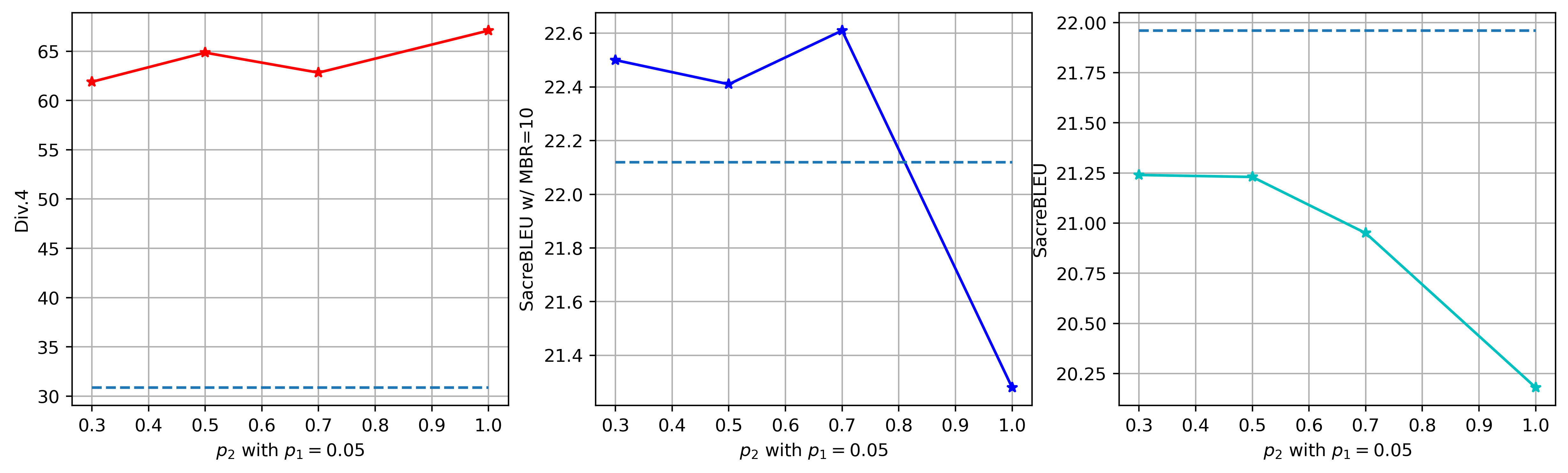
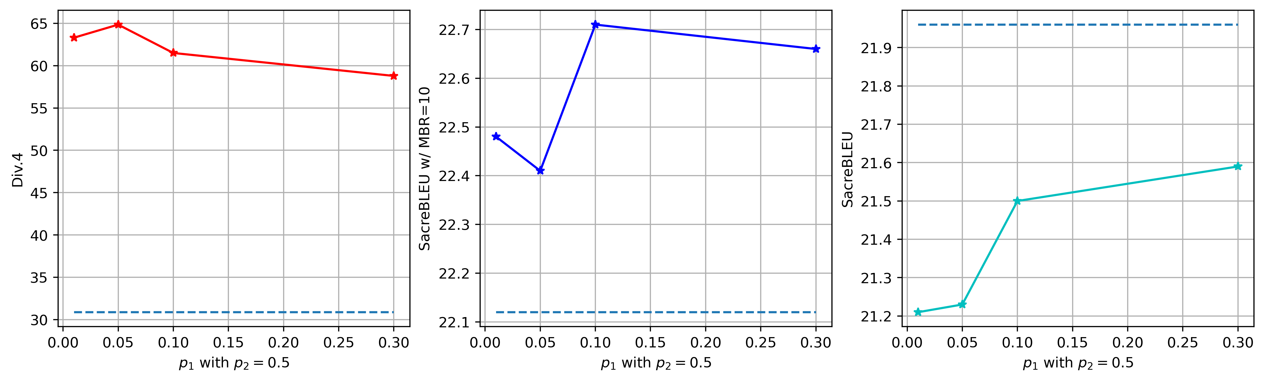
To increase the sequence level diversity, we experiment with randomly replacing the denoising distribution by high variance distribution in Equation 29 in the reverse process during generation. We denote the replacing probability as .
Besides, considering the variance difference between the two sampling distribution are larger at earlier time step in the reverse process, we also explore to only replace the sampling distribution in the first percent of time steps. We generate 10 candidate output sentences for each sample under different random seeds to compute Div.4 and SacreBLEU scores.
As shown in the left subfigure of Figure 4, when fixing the replacing probability to 0.05, the generation diversity are consistently and profoundly improved. In the right subfigure, the generation quality consistently degrades when replacing the denoising distribution when generation, even though the replacing probability is low. In the middle subfigure, we can see that although the generation quality degrades for each candidate, the final output sequences by MBR may improve with proper . In Figure 5, we can get similar results when fixing . In the middle subfigure of Figure 5, the final output sequences are consistently better with different .
To conclude, it is shown that replacing the sampling distribution from the denoising distribution to the prior distribution can provide a trade-off between the generation diversity and generation quality. With a proper combination of and , the generation quality of SeqDiffuSeq with the aid of MBR can be further improved. The benefits of sampling with the prior distribution are always neglected in previous research.
Appendix H More Results on Adaptive Noise Schedule
We present more visualizations of the learned adaptive noise schedules and the losses for each time step on other datasets. Figure 6, 7 and 8 present the visualizations on IWSLT14 EN-DE, QQP, and Wiki-Auto respectively with the same arrangement as Figure 2. The results from the figures are consistent with those discussed in the main texts.


Appendix I Human Evaluation
To better demonstrate the performance of the proposed SeqDiffuSeq , we conduct human evaluations to compare the generated results of SeqDiffuSeq to those of DiffuSeq on the paraphrasing task QQP dataset. We randomly sample 100 data points in the test sets and let annotators decide for the same input sequence, which generated text sequence is better, worse, or of similar quality. We compare SeqDiffuSeq with the previous state-of-the-art text diffusion model DiffuSeq. For fairness, the human evaluations are designed to be blind evaluations (i.e., the annotators are unaware of which model the output sequence is related to).
The human annotators are graduate university students who are proficient in English and are asked to compare the generated sequences based on the following instruction. Decide which generated output sequence is better based on whether the one is more consistent with the input question, whether the one has higher grammatical and syntactic quality. Figure 9 shows the human evaluation results.

The results show that both annotators prefer the generated output sequences by SeqDiffuSeq more. Generated output sequences on QQP from SeqDiffuSeq win by 36% and 44% from two annotators, while those from DiffuSeq only win by 24% and 30% respectively. Human evaluation results show that SeqDiffuSeq can generate text sequences of higher quality than DiffuSeq.
Appendix J Case Study
| Time Step | |
|---|---|
| Input Text | How do I read and find my YouTube comments? |
| 400 | [CLS] how do i read in??? [SEP] [PAD] [PAD] [PAD] [PAD] [PAD] |
| 800 | [CLS] how do i read my a the? [SEP] [PAD] [PAD] [PAD] [PAD] [PAD] |
| 1200 | [CLS] how do i read my youtube comments? [SEP] [PAD] [PAD] [PAD] [PAD] [PAD] |
| 1600 | [CLS] how do i read my youtube comments? [SEP] [PAD] [PAD] [PAD] [PAD] [PAD] |
| 2000 | [CLS] how do i read my youtube comments? [SEP] [PAD] [PAD] [PAD] [PAD] [PAD] |
| Input Text | How do I use Twitter as a business source? |
| 400 | [CLS] how can i use??? a??? [SEP] [PAD] [PAD] |
| 800 | [CLS] how can i use?? as a business?? [SEP] [PAD] [PAD] |
| 1200 | [CLS] how can i use? twitter as a business source? [SEP] [PAD] [PAD] |
| 1600 | [CLS] how can i use? twitter as a business source? [SEP] [PAD] [PAD] |
| 2000 | [CLS] how can i use twitter twitter as a business source? [SEP] [PAD] [PAD] |
| Input Text | What is the funniest joke you know? |
| 400 | [CLS] what is the the tot the you? a? [PAD] [PAD] [PAD] |
| 800 | [CLS] what is the fun?t joke you’for? in? [SEP] |
| 1200 | [CLS] what is the funniest joke you’ve ever know? [SEP] |
| 1600 | [CLS] what is the funniest joke you’ve ever know? [SEP] |
| 2000 | [CLS] what is the funniest joke you’ve ever know? [SEP] |
We select three illustrative cases and investigate the generation process of SeqDiffuSeq. From the cases, it shows that SeqDiffuSeq can generate reasonable text sequences. The generation process reveals that
1. SeqDiffuSeq decides the output sequence length by generating [SEP] tokens at the early stage of sampling;
2. The generation process seems to follow a left-to-right refining order;
3. The position of [SEP] token will not change during sampling, even though there exists token repetition in the generated sequences as shown in red.