Multi-asset market making under the quadratic rough Heston Thanks: This work benefits from the financial support of the Chaires Machine Learning & Systematic Methods. The authors would like to thank Marouane Anane and Alexandre Davroux for very useful comments.
2 Exoduspoint Capital Management, 32 Boulevard Haussmann, 75009 Paris, France
August 11, 2026
Abstract
Given the promising results on joint modeling of SPX/VIX smiles of the recently introduced quadratic rough Heston model, we consider a multi-asset market making problem on SPX and its derivatives, e.g. VIX futures, SPX and VIX options. The market maker tries to maximize its profit from spread capturing while controlling the portfolio’s inventory risk, which can be fully explained by the value change of SPX under the particular setting of the quadratic rough Heston model. The high dimensionality of the resulting optimization problem is relaxed by several approximations. An asymptotic closed-form solution can be obtained. The accuracy and relevance of the approximations are illustrated through numerical experiments.
Keywords— Multi-asset market making, quadratic rough Heston, quadratic approximation
1 Introduction
It is well known that the constant volatility assumption in the celebrated Black-Scholes model is not consistent with empirical observations of financial time series and uneven implied volatility surfaces. Tackling this issue by regarding the volatility as a continuous-time random process, stochastic volatility models are able to reproduce several stylized facts of historical data, such as the fat-tailed distribution of returns and the volatility clustering phenomenon. However, the shapes of the implied volatility surfaces generated by conventional stochastic volatility models, such as the Hull and White, Heston, and SABR models, usually differ substantially from those of empirical observations, see for instance [5]. The rough volatility paradigm brings new solutions, being able to achieve superior fits of implied volatility surfaces than the former models [5, 13, 16]. The recently introduced quadratic rough Heston (QRH) model shows its potential in calibrating jointly SPX and VIX smiles [17]. It models the price of an asset (here the SPX) and its spot variance under risk-neutral measure as
where is a Brownian motion, are all positive constants and is defined as
| (1.1) |
where , , and is a deterministic function. The fractional kernel enables us to generate rough volatility dynamics. It is also used in the rough Heston model, under which the volatility trajectories have almost surely Hlder regularity , for any [14]. This actually recalls the observation in [16] that the dynamic of log-volatility is similar to that of a fractional Brownian motion with Hurst parameter of order 0.1. Importantly, the QRH model gives a natural way to encode the strong Zumbach effect [12], which means that the conditional law of future volatility depends on the past not only through past volatility trajectories but also through past returns.
Note that in this model, only one Brownian motion is involved to generate the stochastic nature of the model and the dynamic of the volatility can be fully explained by past returns. While this is quite different from conventional settings, where volatility is exposed to additional random factors, satisfactory results on market data are reported in [17, 28]. It is also emphasized in [24] that price returns largely explain volatility. An extensive empirical study on the formation process of realized volatility is presented in [29], where the predictive power of price returns on future realized volatility is underlined. The QRH model gives opportunities to model consistently SPX derivatives, including VIX futures, SPX and VIX options. This motivates us to consider a multi-asset market making problem on SPX11 1 SPX, or formally S&P 500 index, is not tradable. When no ambiguity occurs, in this paper it means the liquid index-tracking products such as index funds, ETF, and futures, which are highly correlated with each other. and the aforementioned derivatives of SPX. Today these assets are actively traded and most of the volume comes from electronic trading platforms based on limit order books, which justifies the relevance of developing automated market making algorithms.
The academic literature on optimal market making dates back to the 80s. In [25], the challenge faced by a market maker, which consists in maximizing its profit from spread capturing with a particular focus on execution uncertainty and inventory risk, is formulated as a dynamic programming problem. Approximate solutions are given for specific functional forms of the order arrival rates. The approach is revived in the seminal work [2] with tools of stochastic optimal control. Since then, an extensive literature on optimal market making has been developed. It is shown in [20] that under inventory constraints, the Hamilton-Jacobi-Bellman (HJB) equations associated with the control problem of [2] can be reduced to a linear system of ordinary differential equations (ODEs), for which the asymptotic of the closed-form solution are given when the considered time horizon tends to infinity. Various features, such as model misspecification, short-term alpha signals, and microstructural characteristics, are investigated in [8, 10, 11]. In these papers, a mean-variance type objective function is considered instead of the Von Neumann-Morgenstern expected utility as in [2, 20]. In [19], the results in [20] are extended to more general order execution rates and the two aforementioned objective functions are reconciled. It is shown that the HJB equations associated with the two classes of objective functions can be sorted out into the same family of ODEs.
Multi-asset market making problems are usually exposed to the curse of dimensionality. The conventional grid methods typically used in the case of single-asset become inadmissible given the huge amount of computational resources required. In [7], a method based on factor decomposition is developed to reduce the dimension of the problem. Deep neural networks are considered in [21] to approximate the value function and the optimal quoting strategy. Closed-form approximations are obtained in [6] replacing the Hamiltonian functions with quadratic ones. A similar idea is followed in [4] in the context of option market making. We refer to [9, 18] for a panorama on algorithmic market making.
All the models proposed in the above papers consider continuous control variables, the quotes’ distances with respect to the reference price, which makes them more adapted to quote-driven markets such as corporate bond markets and FX markets. The case of the markets ruled by limit order books is addressed in [22, 23], where the market maker decides whether to submit limit orders at the best limits or to get immediate execution using market orders. More dedicated microstructure models reflecting some important empirical observations at the microstructural scale are chosen in [15, 26].
In this paper, we consider an agent continuously quoting for SPX and its derivatives including VIX futures, SPX and VIX options, via limit orders on both the bid and ask sides. The market maker tries to maximize its expected gain from spread capturing while controlling the inventory risk. In the option market making problems considered in [3, 4], the underlying follows a one-factor stochastic volatility model and perfect Delta hedging is assumed for European options. The market maker then penalizes the option portfolio’s total Vega. In the QRH model, the price dynamics of all the aforementioned derivatives can be explained by the value variation of SPX. Thus, in the context of market making, the principal inventory risk is summarized by the sensitivities of their price change with respect to that of SPX. Even if theoretically this risk can be hedged out perfectly using only SPX as shown in [28], continuous hedging is not realistic and the cost of frequent hedging is far from negligible. More particularly, as the typical inventory process of market making shows a mean reverting behavior around zero, frequent hedging results in unnecessary buys and sells of SPX. In our approach, instead of hedging out completely the net inventory risk of the held derivatives with SPX, the agent also market makes on SPX with limit orders and some net inventory risk is authorized.
The market making basket selected here is essentially made of large tick assets, for which the effective spread is almost always equal to one tick. Thus the quoting strategy of the market maker considered in this paper consists in whether to send limit orders on the two best limits given its portfolio inventory, i.e. whether to make a market on the best limits, instead of choosing the optimal quoting price as most of the models inspired from that of [2]. The resulting modeling framework is in the spirit of [22], while the dimension of the problem is much higher. The high dimensionality comes from two aspects. First, we use here the multi-factor approximation of the QRH model, which is Markovian and suitable for the computation of hedging quantities [1, 28]. However, this brings additional model states. Second, the portfolio of the market maker should be scaled to dozens of assets, including futures and options of various specifications.
To relax the first one, we assume the volatility of SPX and the price sensitivities of other assets against SPX to be constant during the time horizon of market making. At first sight, it seems to deviate from the important feature of the QRH model that volatility spikes can happen in the case of significant price trends. However, this assumption is relevant given the short time horizon of market making problems, which is usually less than several hours. In fact, we always follow the approximated QRH model for the computation of related quantities when switching from one market making period to another, e.g. at the beginning of each day, and we only take them as constant during the following period. As for the multi-asset nature of the problem, we apply the idea introduced in [6] of approximating the HJB equation with another one whose asymptotic closed-form solution can be deduced. Having closed-form approximate solutions makes the recalibration of the algorithm very efficient, and thus it is even possible to design an “online” market making algorithm, i.e. the algorithm is fed regularly with the latest parameter values inside each market making period.
The paper is organized as follows. In Section 2, we recall first the multi-factor approximation of the QRH model, and then describe the considered multi-asset market making problem. Several approximations are introduced in Section 3 to reduce the dimension of the problem. The asymptotic value function associated with the approximated problem is given in closed-form. Finally, in Section 4, we evaluate the relevance of these approximations through numerical experiments.
2 Description of the problem
2.1 Multi-factor approximation of the QRH model
Inspired by [1], in [28] a multi-factor approximation of the QRH model is introduced to make the model Markovian, and an efficient calibration procedure based on deep learning is designed. Essentially, the multi-factor approximation consists in replacing in Equation (1.1) with the approximated kernel function . Then we have
| (2.1) |
and . The parameters are explicit functions of , instead of being free parameters to calibrate, see [28] and the references therein for more details. Now given the Markovian nature of the approximated version of the model, the price of many derivatives of SPX at time , e.g. VIX futures, vanilla SPX and VIX options, can be obtained as a function of . In fact, with being the conditional expectation under the risk-neutral measure, we have the following representations:
- •
VIX future with expiration : with , days.
- •
Vanilla SPX call or put with expiration and strike : or .
- •
Vanilla VIX call or put with expiration and strike : or .
Let denote one of these quantities. Under usual regularity conditions22 2 In practice the price of any derivative concerned here can be approached by a regular approximator, such as the neural network used in [28]., we can write
where
An example with vanilla SPX call is taken in [28] to show the computation of using neural networks. The same approach can be extended to VIX futures and other vanilla options33 3 For SPX we have naturally ..
In [28], the approximation of the pricing mapping is learned directly from samples generated through Monte-Carlo simulations. One can also obtain through solving the following partial differential equation (PDE):
| (2.2) |
with terminal condition , where represents the payoff function of the considered derivative. It is a priori intricate to solve Equation (2.2) with conventional methods, especially when is large. One can apply the method with the help of deep learning introduced in [30], which is reported to be effective on high-dimensional PDEs. For the tests presented in Section 4, we rely on the method introduced in [28] for the computation of .
2.2 Multi-asset market making
Our market making problem is considered over the period , with smaller than the expiration of any asset in our selected basket. For asset , at each point in time, the market maker decides whether to make a market at the limits plus/minus one-half tick size. Let represent the decisions concerning respectively the bid and ask side. The value means the participation of the market maker with a limit order of constant size , and stands for the case where the order is not placed in the queue corresponding to the best limits so that the probability of execution is small. We denote the two point processes modeling the number of transactions at the bid and ask size by and respectively. Then the dynamics of the inventory process of asset is given by
We denote by and the intensity processes of and respectively, which verify
where stands for the maximum inventory of asset that the market maker is willing to hold, which is a multiple of without loss of generality. We do not differentiate the queue positions of the orders in this work, and denote the constant execution probability at the bid and ask side by and respectively.
Denoting by the tick size of asset , the resulting dynamics of the cash process of the market maker is:
Let be the process representing the mark-to-market value of the market maker’s portfolio, i.e. . Its dynamics are given by
The objective function of the market maker considered here is akin to those used in [8, 10, 11], where the expected terminal wealth, i.e. , is maximized while the inventory risk is penalized. More precisely, we are interested in the following optimal control problem:
| (2.3) |
with , , and nonnegative constants. The two items with integration represent the quadratic variation of the inventory risk of individual assets and the portfolio respectively. The market maker can thus consider only the whole portfolio’s net inventory risk () or express also some specific views on the inventory risk of certain particular assets (). Of course, other objective functions can be thought of, such as the widely used constant absolute risk aversion utility function as in [2]. We refer to [19] for a discussion on the equivalence between these two classes of objective functions. Now we can define the value function
associated with (2.3) as
where , , , and
Therefore, has variables. We introduce in the following some approximations to bypass this curse of dimensionality.
3 Value function approximation
3.1 The Hamilton-Jacobi-Bellman equations
To reduce the dimensionality coming from the multidimensional nature of the QRH model, we suggest the following approximation:
Approximation 3.1.
We approximate and by its initial value, i.e.
for . Then we have for by (2.1). We replace the dynamic of by
where and we allow a constant drift .
The above approximation is relevant when the time horizon of the problem is relatively short. In [28] the effectiveness of daily hedging under the QRH model is illustrated through numerical tests on simulated and market data. We give additional daily hedging results in the next section. All these examples indicate that it is reasonable to consider constant at the daily scale. In practice, the market maker can always reset the algorithm with updated parameters in the case of significant market movement. We recall that the computation of and at the beginning of the day is ruled by the QRH model, see [28] for more details. Now the value function satisfies
where
| (3.1) |
Now the value function is transformed to one with variables. Following [27], the HJB equation associated with (3.1) is given by a system of ODEs verifying
| (3.2) |
with terminal condition
| (3.3) |
where is the canonical basis of . We can rewrite the terms involving the control variables as
with
| (3.4) |
In the following we give the results on the existence and uniqueness of a solution of (3.2) with terminal condition (3.3). We give the sketch of the proof as it follows the same steps as in [19].
Theorem 3.1.
Proof.
It is clear that are Lipschitz continuous functions for all and . Equation (3.2) with terminal condition (3.3) can be viewed as a backward Cauchy problem. According to the Cauchy-Lipschitz theorem, there exists some such that the Equation (3.2) with the terminal condition (3.3) has a unique solution, in time, on the interval .
, it is clear that the function is a decreasing function. Therefore, the only reason why there would not be a global solution on is because blows up at . By the fact that is decreasing, a classical comparison principle can be obtained. It is clear that defines a supersolution of (3.2) with terminal condition (3.3). Then by the comparison principle, we have
This shows that is bounded for , which leads to its existence and uniqueness on . ∎
By a classical verification argument, we can get the following result:
Theorem 3.2.
Remark 3.1.
When the market maker controls only the portfolio’s net risk, i.e. and , the -dimensional variable can be summarized with one variable. More precisely, by introducing the maximum risk bound and , now the value function associated with the problem can be written as
| (3.5) |
And the associated HJB equation is given by
with terminal condition .
3.2 Quadratic approximation
In our case with a portfolio made of SPX and numerous derivatives, Equation (3.2) becomes intricate to solve with classical numerical methods. Here we follow the idea of [6] that is approximating the Hamiltonian functions with quadratic ones. Then closed-form solution can be obtained for the new HJB equation. Moreover, the asymptotic of the solution can be derived, which are helpful for practical use. Note that most of the development in this part follows the same methodologies as in [6]. We give some key results in the following to avoid any ambiguity.
The market making problem considered in [6] is more adapted to over-the-counter market, where the optimal control is the quoting price and is taken to be continuous. The resulting Hamiltonian functions are and a natural choice is to use Taylor expansions as the approximations. Clearly this do not apply for (3.4). In this work we propose the following choice as the approximated Hamiltonian functions:
| (3.6) |
with . Actually we have and for any . We can choose to make close to around . In the case without maximal inventory constraints for individual assets, i.e. , following the same computations as in [6], the approximation of associated with , denoted by , can be written as a quadratic function of , i.e.
where and are given by the unique solution of a system of ODEs44 4 We denote by the set of positive semi-definite symmetric matrices of dimension .. Since we are more interested in the behavior of as , we focus mostly on the asymptotic formulas of and 55 5 We ignore since it is irrelevant for the dependence of the value function on the states.. Let and . We have
where
is the Moore-Penrose inverse of and is the linear operator mapping a matrix onto the vector of its diagonal coefficients. As we focus on the asymptotic of the approximated solution in the following, we use and to represent the respective asymptotic formulas for ease of notation. As suggested in [6], for any , one important application of is to make greedy decisions following
It is clear that the set and are separated by an affine hyperplane defined on . In the particular case with only portfolio-level net risk controlled, as suggested in Remark 3.1, and symmetric order execution intensities on the bid and ask sides, i.e. for all , applying the above quadratic approximation on Equation (3.1), the optimal decisions can be simplified as
where
Remark 3.2.
In the market making problem introduced in Section 2.2, the agent is restricted to sending limit orders only on the first bid and ask limits. The problem can be easily extended to cover other limits. The resulting Hamiltonian functions can also be approximated and then a closed-form asymptotic solution can be obtained in a similar manner as the above.
4 Numerical results
4.1 Daily hedging with SPX
In this part, we perform discrete hedging to evaluate the relevance of the QRH model and the idea of using constant during a short period, as suggested in Approximation 3.1. For asset , the cumulative profit of discrete hedging with a time step is given by
where , , and is the hedging quantity at computed by neural networks. We compare with the price evolution of asset observed in the market, defined by
Figure 4.1 and 4.2 show the results of two experiments of daily hedging on SPX call, VIX call and VIX future with the following characteristics:
- 1.
SPX call: maturity 2017-07-21, strike 2460; VIX call: maturity 2017-07-19, strike 11.5; VIX future: maturity 2017-07-19.
- 2.
SPX call: maturity 2017-10-20, strike 2550; VIX call: maturity 2017-10-18, strike 13; VIX future: maturity 2017-10-18.
On day zero of each experiment, we calibrate the QRH model with market data and compute . For each following day, are updated with respect to the evolution of SPX, and then are recomputed. Remarkably in both tests, the hedging portfolios can follow well the market price’s evolution with daily rebalancing for all assets. It implies that in practice high-frequency hedging is not mandatory to obtain satisfactory results, and verifies the rationality of Approximation 3.1 over the time horizon of the considered market making problem, which is usually shorter than one day.
4.2 Market making approximation
4.2.1 Example 1
In this part, we assess the proposed quadratic approximation. We begin with a two-asset example with SPX and VIX future. The parameters of the QRH model are taken as follows66 6 The same multi-factor approximation method as that in [28] is used, leading to the same and :
Then we have . We set $, and . The maturity of VIX future is set to be one month. Along with , using the neural network approximating the pricing function of VIX future, we have .
As for the market making related parameters, we consider the following values:
- •
Tick size:
- •
Order size:
- •
Maximum inventory:
- •
Execution intensity:
- •
Risk penalization:
- •
Time horizon: .
Here some characteristics of SPX are referred to the front month E-mini S&P 500 future. In real life, the contract multiplier of E-mini S&P 500 future is 50, and that of VIX future is 1000. Here we normalize them against 50 to have order sizes. The execution intensities are selected such that on average the volume of SPX is 10 times that of VIX future.
First, we use a classical Euler scheme to approximate numerically the true value function . Figure 4.3 shows the results for several . Interestingly, the shapes of at different are very similar, implying that time does not play a crucial role for the optimal controls according to Theorem 3.2. This is confirmed by Figure 4.4, showing that for SPX or VIX future, the set does not change a lot with when is relatively small.
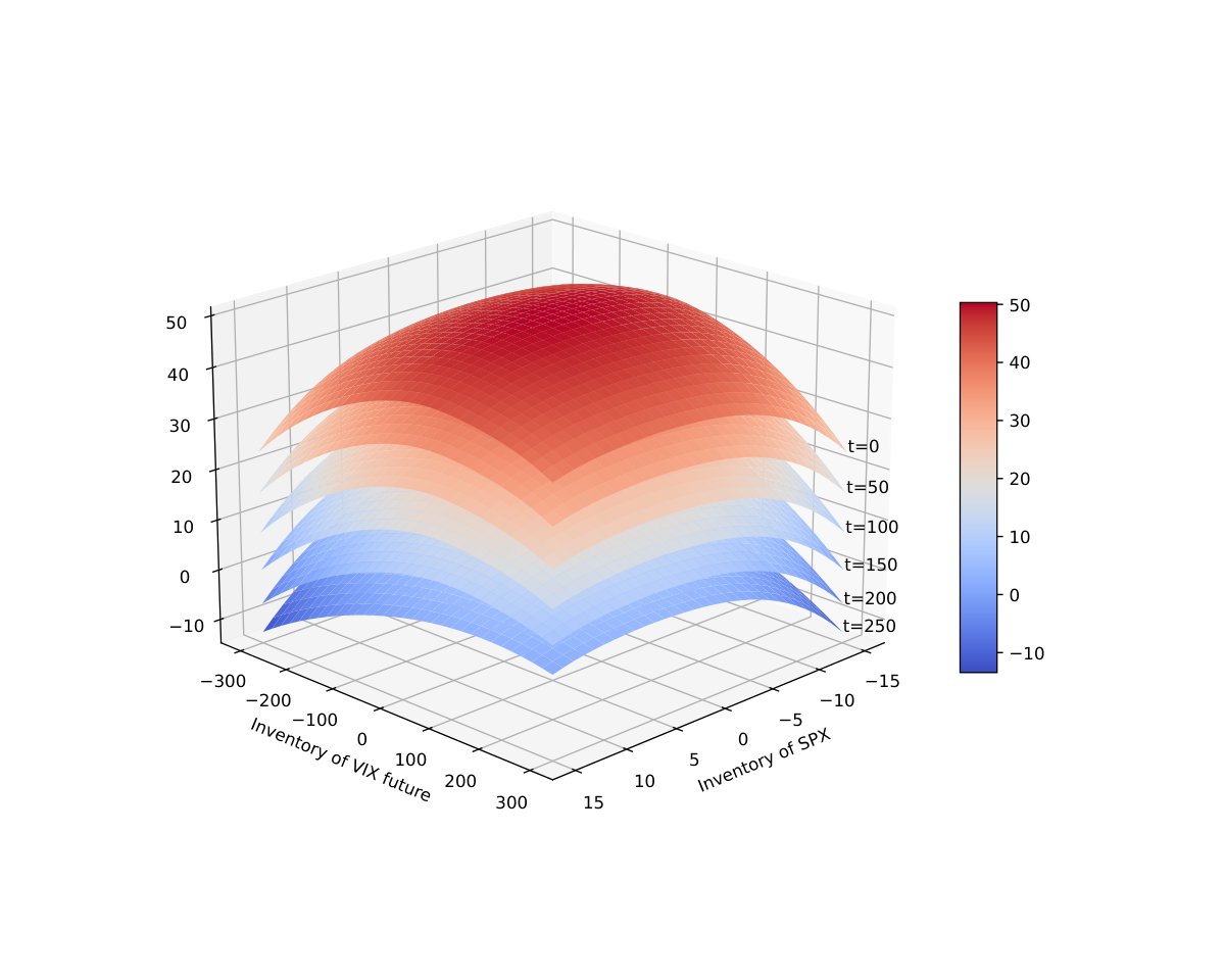
Now we check the relevance of our quadratic approximation. As for the parameter defined in Equation (3.6), we choose . The asymptotic approximated value function is shown in Figure 4.5. Its shape is very close to that of , and the resulting greedy decision , given in Figure 4.6, is very similar to shown in Figure 4.4.

To see the impact of the quadratic approximation in cases with other values of and , and to quantify the deviation of the market making decisions following the approximated solution from the ones based on the true solution, we conduct backtests on simulated data with different risk aversion preferences77 7 Our simulations use neural networks to compute efficiently the price of SPX and VIX option, and VIX Future as introduced in [28].. More precisely, we vary the inventory penalization parameter from to and fix for simplicity. We test two strategies and , based respectively on and 88 8 For ease of notation, we ignore the superscript in the following.. For each pair and , we evaluate the mean and standard deviation of the profit of market making, defined as where stands for the backtesting horizon, on simulated paths. We use seconds as the backtesting horizon since we are more interested in the results given by the asymptotic of . With , Figure 4.7 shows the resulting mean-risk profiles for and . Even though for a given , slight deviations from are observed for , the global mean-risk profile of its performance is not significantly degraded from that of . This suggests the effectiveness of the proposed approximation method.
4.2.2 Example 2
Here we repeat the same experiment as the above for the case where only the portfolio’s net inventory risk is controlled, as discussed in Remark (3.1). We consider the following assets:
- •
SPX option with maturity days and strike .
- •
SPX option with maturity days and strike .
- •
VIX option with maturity days and strike .
- •
VIX option with maturity days and strike .
And we have the following parameters:
- •
Tick size: .
- •
Inventory risk: .
- •
Order size: for .
- •
Inventory risk bound: .
- •
Execution intensity: for .
- •
Risk penalization: .
- •
Time horizon: seconds.
With four assets under consideration, the value function defined in Equation (3.5) can be solved with classical Euler scheme based on grids. As shown in the left subfigure of Figure 4.8, the shape of the slices is very stable through time. We then apply the above quadratic approximation method and obtain its asymptotic form as , which is shown to be very close to in Figure 4.8.
Similarly to the above example, we use backtests to perceive more directly the effectiveness of the approximated solution. We choose seconds and for each pair and , the mean and standard deviation of the performance on paths are computed. Figure 4.9 shows the results with varied from to . We remark again that the mean-risk profile of is very close to that of .
4.3 Example 3
In this part we consider a market making problem on the six assets mentioned above to exemplify the effect of risk mutualization among them. We test with seconds, varying from to and . As indicated in the introduction, having a closed-form asymptotic solution allows us to recalibrate instantly the solution with the most recently observed parameters. To illustrate the idea, during the test we update and every 100 seconds according to the running state of the QRH model, i.e. . As for the benchmarking case, we set so that the inventory risk of each asset is managed individually. Classical Euler scheme is used for solving the value function of each asset, and then the corresponding optimal decisions can be obtained. Figure 4.10 gives the results on 5000 simulated paths. Clearly, the performance of uni-asset market making is suboptimal compared to the other setting, which also considers the net risk at the portfolio level.
References
- [1] E. Abi Jaber and O. El Euch. Multifactor approximation of rough volatility models. SIAM Journal on Financial Mathematics, 10(2):309–349, 2019.
- [2] M. Avellaneda and S. Stoikov. High-frequency trading in a limit order book. Quantitative Finance, 8(3):217–224, 2008.
- [3] B. Baldacci, P. Bergault, and O. Guéant. Algorithmic market making for options. Quantitative Finance, 21(1):85–97, 2021.
- [4] B. Baldacci, J. Derchu, and I. Manziuk. An approximate solution for options market-making in high dimension. Risk, June, 2021.
- [5] C. Bayer, P. Friz, and J. Gatheral. Pricing under rough volatility. Quantitative Finance, 16(6):887–904, 2016.
- [6] P. Bergault, D. Evangelista, O. Guéant, and D. Vieira. Closed-form approximations in multi-asset market making. Applied Mathematical Finance, 28(2):101–142, 2021.
- [7] P. Bergault and O. Guéant. Size matters for OTC market makers: general results and dimensionality reduction techniques. Mathematical Finance, 31(1):279–322, 2021.
- [8] Á. Cartea, R. Donnelly, and S. Jaimungal. Algorithmic trading with model uncertainty. SIAM Journal on Financial Mathematics, 8(1):635–671, 2017.
- [9] Á. Cartea, S. Jaimungal, and J. Penalva. Algorithmic and high-frequency trading. Cambridge University Press, 2015.
- [10] Á. Cartea, S. Jaimungal, and J. Ricci. Buy low, sell high: A high frequency trading perspective. SIAM Journal on Financial Mathematics, 5(1):415–444, 2014.
- [11] Á. Cartea, S. Jaimungal, and J. Ricci. Algorithmic trading, stochastic control, and mutually exciting processes. SIAM review, 60(3):673–703, 2018.
- [12] A. Dandapani, P. Jusselin, and M. Rosenbaum. From quadratic Hawkes processes to super-Heston rough volatility models with zumbach effect. Quantitative Finance, 21(8):1235–1247, 2021.
- [13] O. El Euch, J. Gatheral, and M. Rosenbaum. Roughening Heston. Risk, pages 84–89, 2019.
- [14] O. El Euch and M. Rosenbaum. The characteristic function of rough Heston models. Mathematical Finance, 29(1):3–38, 2019.
- [15] P. Fodra and H. Pham. High frequency trading and asymptotics for small risk aversion in a markov renewal model. SIAM Journal on Financial Mathematics, 6(1):656–684, 2015.
- [16] J. Gatheral, T. Jaisson, and M. Rosenbaum. Volatility is rough. Quantitative finance, 18(6):933–949, 2018.
- [17] J. Gatheral, P. Jusselin, and M. Rosenbaum. The quadratic rough Heston model and the joint S&P 500/VIX smile calibration problem. Risk, May, 2020.
- [18] O. Guéant. The Financial Mathematics of Market Liquidity: From optimal execution to market making, volume 33. CRC Press, 2016.
- [19] O. Guéant. Optimal market making. Applied Mathematical Finance, 24(2):112–154, 2017.
- [20] O. Guéant, C.-A. Lehalle, and J. Fernandez-Tapia. Dealing with the inventory risk: a solution to the market making problem. Mathematics and financial economics, 7(4):477–507, 2013.
- [21] O. Guéant and I. Manziuk. Deep reinforcement learning for market making in corporate bonds: beating the curse of dimensionality. Applied Mathematical Finance, 26(5):387–452, 2019.
- [22] F. Guilbaud and H. Pham. Optimal high-frequency trading with limit and market orders. Quantitative Finance, 13(1):79–94, 2013.
- [23] F. Guilbaud and H. Pham. Optimal high-frequency trading in a pro rata microstructure with predictive information. Mathematical Finance, 25(3):545–575, 2015.
- [24] J. Guyon and J. Lekeufack. Volatility is (mostly) path-dependent. Available at SSRN 4174589, 2022.
- [25] T. Ho and H. R. Stoll. Optimal dealer pricing under transactions and return uncertainty. Journal of Financial economics, 9(1):47–73, 1981.
- [26] X. Lu and F. Abergel. Order-book modeling and market making strategies. Market Microstructure and Liquidity, 4(01n02):1950003, 2018.
- [27] B. Øksendal and A. Sulem. Stochastic control of jump diffusions. Springer, 2005.
- [28] M. Rosenbaum and J. Zhang. Deep calibration of the quadratic rough Heston model. Risk, October, 2022.
- [29] M. Rosenbaum and J. Zhang. On the universality of the volatility formation process: when machine learning and rough volatility agree. arXiv preprint arXiv:2206.14114, 2022.
- [30] J. Sirignano and K. Spiliopoulos. DGM: A deep learning algorithm for solving partial differential equations. Journal of computational physics, 375:1339–1364, 2018.