Uncertainty Quantification of MLE for Entity Ranking with Covariates
Abstract
We study statistical estimation and inference for the ranking problems based on pairwise comparisons with additional covariate information. In specific, in this paper, we study a Covariate-Assisted Ranking Estimation (CARE) model in a systematic way, that extends the well-known Bradley-Terry-Luce (BTL) model by incorporating the covariate information. We impose natural identifiability conditions, derive the statistical rates for the MLE under a sparse comparison graph, and obtain its asymptotic distribution. Moreover, we validate our theoretical results through large-scale numerical studies.
keywords
High-Dimensional Inference, Entity ranking, Ranking with covariates, Uncertainty quantification, Maximum likelihood estimator.1 Introduction
Ranking plays an essential role in many real-world applications. For example, it is crucial in individual choice (Luce 2012), psychology (Thurstone 1927; Thurstone 2017), recommendation systems (Baltrunas et al. 2010; Li et al. 2019), and many others. The ranked items such as sports teams (Massey 1997; Turner and Firth 2012), scientific journals (Stigler 1994), web pages (Dwork et al. 2001), election candidates (Plackett 1975), or even movies (Harper and Konstan 2015) will not only illustrate their qualities but also affect people’s future choices. Thus, the ranking problem has been extensively studied in statistics, machine learning, operations research, etc.; see, for example, (Hunter 2004; Richardson et al. 2006; Jang et al. 2018; Chen et al. 2019; Chen et al. 2022b; Chen et al. 2022a; Liu et al. 2022) for more details.
Among various models for the ranking problem, the most well-known one is the Bradley-Terry-Luce (BTL) model (Bradley and Terry 1952; Luce 2012), which assumes the existence of scores of compared items such that the preference between item and item is given by
The underlying assumption of this BTL model is the scores of compared items are fixed and do not explicitly use their attributes. However, in many real-world applications, covariate information often exists and this heterogeneity needs to be incorporated. For example, US News and Times Higher Education consider many characteristics of universities, such as international research reputation, teaching quality, the ratio between students and professors, and citations to conduct global university rankings. In addition, in NBA basketball competitions, the final rank of a team is also affected by its underlying attributes, such as the ability to defend, make a three-point shot, etc.
Thus, a crucial question still remains open:
“Can one design a provably efficient mechanism for ranking by incorporating features of compared items and conduct associated high-dimensional statistical inference?”
To this end, we follow the idea from related literature (Turner and Firth 2012; Li et al. 2022), by incorporating feature information of items into the BTL model, and call the model the Covariate-Assisted Ranking Estimation (CARE) model. Specifically, we address covariate heterogeneity by assuming the underlying score (ability) of the -th item is given by , where captures the covariate effect and is the intrinsic score that cannot be explained by the covariate. In this case, the outcome of pairwise comparison is modeled as
We do not assume that all pairs are compared. Rather, each pair is selected at random for comparison. In specific, we let the underlying comparison graph be a realization of the Erdős-Rényi random graph with edge probability . In addition, once a pair is selected, they are compared times. This can be two teams matching times or two universities ranked times by experts. In this work, we consider the fixed design in the sense that the randomness only comes from results of comparisons.
There are several challenges in studying statistical inference for our CARE model. First, our model incorporates feature information into the original BTL model, not only the underlying scores but also shall be estimated and analyzed in a novel way. This also gives rise to the issue of identifiability. Second, given consistent estimators, it remains open to quantifying these key components’ uncertainty. Most existing work focuses more on deriving statistical rates of convergence for those underlying scores via various estimators in the BTL model to achieve specific rank recoveries such as top-K and partial recovery (Chen et al. 2019; Chen et al. 2022b). There are few results established for the inference of the BTL model (Simons and Yao 1999; Han et al. 2020; Gao et al. 2021; Liu et al. 2022), letting alone the uncertainty quantification for the more general BTL model with covariates (CARE model).
In our work, we resolve the first challenge by designing a novel constrained maximum likelihood estimator (MLE) which efficiently estimates the underlying scores and . With some proper initialization, the MLE can be solved by simply running the projected gradient descent algorithm. By leveraging the ‘leave-one-out’ technique (Chen et al. 2019), we prove that the statistical rate of convergence of the MLE of the intrinsic scores and overall scores in -norm are of order and , respectively, in which is the dimension of the observed covariates. These statistical rates reduce to the standard minimax rates for estimating the BTL model when no covariate exists, (Chen et al. 2019).
To take on the second challenge, namely, depicting the asymptotic distribution of the MLE, we first approximate the MLE by the minimizer of the quadratic approximation of our joint likelihood function, whose uncertainty is easier to depict. The critical difficulty lies in quantifying this approximation error. To tackle this issue, we then utilize the ‘leave-one-out’ technique and derive novel proofs, which is valid under the minimal sample complexity up to logarithm terms. In a more specific BTL model, the seminal works by Gao et al. 2021 and Fan et al. 2024+ (when considering pairwise comparison) leverage the minimizers of the more restricted diagonal quadratic approximations of their marginal likelihoods to approximate the MLE. They capture the approximation errors based on a ‘leave-two-out’ technique. In contrast, in this work, we utilize the minimizer of the quadratic approximation of the joint likelihood to approximate the MLE, and achieve a tighter approximation error than Gao et al. 2021; Fan et al. 2024+.
Finally, we conduct numerical experiments to corroborate our theory. The performance of the model is also convincingly illustrated by an analysis of the data on Pokemon competitions. From the perspective of stock selection and return prediction, our proposed covariate-assisted BTL model (CARE) outperforms the original BTL model in many aspects.
To summarize, the contributions of this work are of multiple folds. First, we study a Covariate-Assisted Ranking Estimation (CARE) model in a systematic way that extends the well-known Bradley-Terry-Luce (BTL) model by incorporating the covariate information. Specifically, we derive - and - statistical rates for the MLE of and , respectively. Moreover, we also conduct uncertainty quantification for our MLE, where we improve the approximation errors given in existing works and derive more general asymptotic results. Furthermore, our results hold even on the sparse comparison graph, i.e. the probability of pairwise comparison up to logarithm terms, with minimal sample complexity. Finally, we illustrate our methods via large-scale numerical studies on synthetic and real data. Numerical results lend further support to our proposed CARE model over the original BTL model.
1.1 Prior Arts
Ranking problems based on pairwise comparison for parametric and non-parametric models have received much attention. For the BTL model, Hunter 2004 studies its variants and establishes theoretical properties using a minorization-maximization algorithm. Chen and Suh 2015 use a two-step method to study the BTL model, which is provably optimal in terms of sample complexity. Jang et al. 2016 leverage the spectral method to recover the top-K items with only minimal samples. In addition, Negahban et al. 2012 propose an iterative rank aggregation algorithm named Rank Centrality to recover the underlying scores of the BTL model in optimal - statistical rate. In the sequel, Chen et al. 2019 derive both - and - optimal statistical rates of those underlying scores and prove that the regularized MLE and spectral method are both optimal for recovering top-K items when the conditional number is a constant. Furthermore, Chen et al. 2022b proves that for partial recovery, MLE is optimal, but the spectral method is not when we have a general conditional number. It is worth noting that the aforementioned prior arts mainly focus on studying the parametric BTL model. There is also a series of works that studies specific non-parametric variants of the BTL model. For instance, Shah and Wainwright 2017 develop a counting-based algorithm to recover top- ranked items under the nonparametric stochastically transitive model. For more details on the non-parametric comparison models, see Shah et al. 2016; Shah and Wainwright 2017; Chen et al. 2017; Pananjady et al. 2017 and the references therein.
Going beyond the pairwise comparison, there also exist other works that study ranking problems using -way comparisons . The first well-known model is the Plackett-Luce model and its variants (Plackett 1975; Guiver and Snelson 2009; Cheng et al. 2010; Hajek et al. 2014; Maystre and Grossglauser 2015; Szörényi et al. 2015; Jang et al. 2018; Fan et al. 2024+). For instance, a closely related work is Jang et al. 2018, who study the Plackett-Luce model under a uniform hyper-graph. They divide -way compared data into pairs and utilize the spectral method to derive the - statistical rate of underlying scores. They further provide a lower bound for sample complexity to recover top-K items in the Plackett-Luce model. Another well-known model is the Thurstone model (Thurstone 1927), which admits the Plackett-Luce model as a particular case; see Thurstone 1927; Guiver and Snelson 2009; Hajek et al. 2014; Vojnovic and Yun 2016; Jin et al. 2020 for more details.
The aforementioned literature mainly focuses on non-asymptotic statistical consistency results for the underlying scores of compared items through various ranking frameworks. However, the limiting distributional results for ranking models still remain highly under-explored. There are several results on the asymptotic distributions for the ranking scores in the BTL model. For instance, Simons and Yao 1999 derive the asymptotic normality of the MLE of the BTL model in the scenario where all pairs of comparison are fully conducted (i.e., ). Han et al. 2020 further extend the results to the regime where the comparison graph (Erdős-Rényi random graph) is dense but not fully connected, i.e., . In addition, recently, Liu et al. 2022 propose a Lagrangian debiasing method to derive asymptotic distribution for ranking scores, where they allow sparse comparison graph but require comparison times to be larger than Moreover, Gao et al. 2021 utilize a ‘leave-two-out’ trick to derive asymptotic distributions for ranking scores with optimal sample complexity in the regime where the comparison graph is sparse, i.e., up to logarithm terms.
All aforementioned models and methods mainly study the estimation and uncertainty quantification for ranking models without considering any individual feature information. Yet, covariate data exist in most applications, and this results in additional challenges in technical derivations and computation. Although there exists some other literature that also considers incorporating covariate information into the ranking problems (Guo et al. 2018; Schäfer and Hüllermeier 2018; Zhao et al. 2022; Chau et al. 2023; Finch 2022), their motivations, model settings, methodology, and theoretical contributions are different from us. In specific, most of them assume the underlying scores of all compared items are fully explained by covariates without studying the effects of individual intrinsic scores (i.e., no ). In addition, we allow the comparisons to be realized through (sparse) comparison graphs, which take on extra challenges. Moreover, in terms of the theoretical contribution, most of them only establish the - statistical rates for estimating whereas we not only obtain -and - statistical rates for estimators of and but quantify their uncertainty as well. In addition, even though our CARE model is related to Turner and Firth 2012; Li et al. 2022, we propose a systematic model estimation and inference framework. In contrast, these previous works only formulate ranking with covariates intuitively and do not discuss methodological implementations or theoretical guarantees.
Therefore, this paper takes up this challenge by presenting a systematic framework for model estimation and uncertainty quantification of our CARE model over a random comparison graph. Notably, this framework admits all previous advancements made on the BTL model, which do not incorporate covariate information as special cases.
1.2 Notation
We introduce some useful notations before proceeding. We denote by for any positive integer . For any vector and , we use to represent the vector norm of . In addition, the inner product between any pair of vectors and is defined as the Euclidean inner product . For vector and index , we denote by the vector we get by deleting the -th element in . For any given matrix , we use , , and to represent the operator norm, Frobenius norm, nuclear norm and two-to-infinity norm of matrix respectively. Moreover, we use or to denote positive semidefinite or negative semidefinite of matrix . Moreover, we use the notation or for non-negative sequences and if there exists a constant such that . We use the notation for non-negative sequences and if there is a constant such that . For simplicity, we define function . We write if and . For matrix , we denote by its pseudoinverse (Banerjee 1973).
1.3 Roadmap
The remaining paper is organized as follows. We describe the problem formulation for our BTL model with covariate and derive the corresponding maximum likelihood estimators for its involved parameters in §2. In §3, we establish the statistical estimation results for our MLE. In §4, we further conduct uncertainty quantification for the obtained MLE. In §5, we corroborate our theoretical results by conducting large-scale numerical studies via both synthetic and real dataset.
2 Model Formulation
In this section, we introduce the Covariate-Assisted Ranking Estimation (CARE) model, which incorporates covariate information into the BTL model. In the traditional BTL model (Bradley and Terry 1952; Luce 2012), it is assumed that each item has a latent score and the outcomes of comparisons are modeled as the realizations of the Bernoulli trials:
| (1) |
It is worth mentioning that the function in (1) can be replaced by any increasing differentiable functions.
In many applications, one observes individual features and would like to incorporate them for conducting more accurate ranking. As an extension of the parameterization (Chen et al. 2019; Chen et al. 2022b), we model the scores as for . The linear term captures the part of the scores explained by the variables and represents the intrinsic score that can not be explained by the covariate . This leads to modeling the outcomes of comparisons as the Bernoulli trials with probabilities
| (2) |
We call this model Covariate Assisted Ranking Estimation (CARE) model.
We do not assume that all pairs are compared, but only those in the comparison graph . Here and represent the collections of vertexes ( items) and edges, respectively. More specifically, if and only if item and item are compared. Throughout our paper, the comparison graph is assumed to follow the Erdős-Rényi random graph (Erdos et al. 1960) where each edge appears independently with probability . In short, items i and j with are compared at random with probability .
In addition, for any , we observe independent and identically distributed realizations from the Bernoulli random variables
Let and , where stand for the canonical basis vectors in and Then, the log-likelihood function conditioned on is given by
where is a sufficient statistic. The identifiability question arises naturally since we over-parametrized the problem. To remedy this issue, we restrict the parameter space of onto some constrained set with a natural interpretation. In specific, we denote let and consider the constrained set . Throughout the paper, we assume that has rank . Under these identifiability constraints, if the true parameter vector , the identifiability condition implies that and with . It admits clear interpretation: represents the scores that be captured by the covariates, whereas the represents the residual scores (or equivalently intrinsic scores) that can not be explained by the involved features (i.e., it is orthogonal to the linear space spanned by the columns of covariates). Next, we prove the identifiable property of rigoriously in Proposition 1.
Proposition 1.
CARE model Eq. (2) with parameter space is identifiable.
We denote by a matrix by padding matrix to , i.e. and . As a result, can be also written as . Denote by the projection matrix onto space .
Given the aforementioned identifiable condition, we consider the following constrained maximum likelihood estimator (MLE)
| (3) |
where
| (4) |
Note that when there is no covariate , we have and the scores are identifiable up to a constant shift. Therefore, our formulation includes those studies of the BTL model without covariate information as special cases (Chen et al. 2019).
The inference question arises naturally if some covariates can explain the underlying scores, namely if some or all components of are statistically significant. Similarly, one might ask if the covariates are adequate for determining the underlying scores by testing whether some or all components of are zero. In general, we would expect the variations among the components of to be smaller than the original scores . This enables us to improve data predictions by shrinking or regularizing the estimate of
In the following context, we rescale to , where is a positive number such that for all after the transformation. The likelihood function, prediction and the column space spanned by are not affected by the scaling but this normalization facilitates us with scaling issues in the technical derivations. Therefore, the content that follows will be based on the scaled data and parameters.
3 Rate of Convergence of Maximum Likelihood Estimator
In this section, we show the statistical consistency results for the maximum likelihood estimator in (3). Before proceeding to the main results, we begin by introducing several key assumptions on the design matrix. First, we assume the projected matrix satisfies the following incoherence condition. {assumption}[Incoherence Condition] Assume that there exists a positive constant such that
To demonstrate the rationality behind Assumption 3, we first note that the . Therefore, a sufficient condition for this assumption to hold is when the rows of are nearly balanced, with row sum of squares all of the order or smaller. When there does not exist the covariate (i.e. ), we have In this scenario, this assumption holds automatically with The following results of this paper are established under this incoherence condition.
We next introduce a key assumption on the covariates which guarantees a well-behaved landscape of the loss function as well as good statistical properties of the MLE estimator. In specific, we put the following assumption on .
Assume that there exist positive constants and such that
where is the operator norm of and
In this Assumption 3, we assume that is well-behaved in all directions inside our parameter space , namely, both of its largest and smallest eigenvalues are of order . This assumption follows directly after we rescale the such that for all . When there is no covariate (i.e., ), then and Assumption 3 holds naturally with (Chen et al. 2019).
We next introduce the condition number of this problem as
where , which extends the condition number in Chen et al. 2019 when there does not exist covariate. With all aforementioned assumptions in hand, we next present our first main theorem on the statistical rates of convergence of the MLE . Recall that we assume that the true parameter vector , without loss of generality.
Theorem 2.
(Rate of convergence) Suppose for some and . Consider for any absolute constants . Let be the solution of the MLE given in (3). Then with probability at least , we have
where .
Recall that we rescaled the covariates such that . This scaling has an impact on the definition of and influences its rate. This explains why converges slower and does not depend on . However, when we view as a whole, the estimation rate is , and this does not impact the estimation of the individual score, as shown in Theorem 2.
Remark 3.
Following a similar proof, it holds that
which are the relative -statistical rates of the intrinsic scores and overall scores , respectively. Combining this relative statistical rate in -norm with that in -norm mentioned in Theorem 2, we conclude that the estimation errors of latent scores and overall scores spread out across all items.
Remark 4.
We note that we are further able to get rid of the factor in the statistical rates of ( follows directly). This involves analyzing the non-asymptotic expansion of the , and the details will be discussed in the following section.
4 Uncertainty Quantification of MLE
Most existing works on ranking mainly study the first-order asymptotic behavior of their estimators (Hunter 2004; Chen and Suh 2015; Jang et al. 2016; Shah and Wainwright 2017; Chen et al. 2019). Deriving limiting distributional results in ranking models is important for uncertainty quantification, especially when covariate information is incorporated into the ranking problem, are not studied in detail.
This section is devoted to understanding the sampling variability of the MLE under the CARE model. Directly studying the asymptotic behavior of is very challenging. To address this issue, we approximate by considering
| (5) |
here is the quadratic expansion of the loss function around given by
| (6) |
According to this definition, can also be given by the following linear equations
Here represents the linear projection onto space Observe that serves as a candidate approximator of whose uncertainty is easier to quantify according to Berry-Esseen theorem (Berry 1941; Esseen 1942). It is not a statistical estimator but an auxiliary random variable that we used for the technical proof. It is worth mentioning that when there is no covariate, our linear expansion reduces to which is equal to the expansion in Gao et al. 2021 up to the off-diagonal terms in
The critical difficulty falls in proving that the difference is negligible compared to under certain conditions. To accommodate this, we derive novel proofs by leveraging the ‘leave-one-out’ (Chen et al. 2019; Chen et al. 2021) technique to control the approximation error in -norm and in -norm. The upper bounds are summarized in the following Theorem 5.
Theorem 5.
(Approximation error) Under the assumptions of Theorem 2, if and for some fixed constant , we have
and with probability at least it holds that
Remark 6.
The assumptions and for some fixed constant are mild. When and are bounded, they hold when . This matches the lower bound of the sampling probability to ensure the connectivity of the Erdős-Rényi random graph, which is a necessary requirement for item ranking. Besides, is also required by the consistency results of our estimator according to Theorem 2.
Remark 7.
Given the non-asymptotic expansion, and approximation error presented in Theorem 5, we are able to achieve a tighter statistical error bound for Specifically, under the assumptions of Theorems 4 and 7, as long as
Then with probability at least we have
Next, we utilize Berry-Essen theorem (Berry 1941; Esseen 1942) to derive the asymptotic distribution of the linear combinations of , respectively. Since it holds for any linear combinations, the result applies to any finite-dimensional distribution of .
Theorem 8.
(Asymptotic normality of MLE) Given , let be the projection of onto linear space . Under the assumptions of Theorem 5, we have the following decomposition
where
with probability exceeding (randomness comes from and ) and
with probability exceeding (randomness comes from ). Combining the approximation error and asymptotic distribution together, and by taking all randomness into consideration, we further obtain
In Theorem 8, we first obtain the distributional guarantee of , conditioned on the comparison graph , in the sense that we only take the randomness of into consideration. These results are stronger than the distributional guarantees, which make use of all the randomness from and , by the dominated convergence theorem. Besides, combining with the approximation results, we further derive distributional guarantees for linear combinations of by taking all the randomness of into consideration. The asymptotic variance of is as presented in Theorem 8, where is exactly the inverse of the fisher information (conditioned on graph ) that is projected into the space .
Moreover, recall that we have scaled the covariates to satisfy in the data preprocessing step. Then, if and are bounded, the asymptotic normality holds when
| (7) |
in the sense that it allows the comparison graph to be sparse (when up to logarithmic terms) when the covariate dimension is bounded. This admits all existing uncertainty quantification results for the BTL model without covariates as special cases.
Finally, we comment on the condition . This is only a mild requirement. For instance, when and is sparse (the original BTL model), this inequality holds naturally. In addition, the comparison of preference ratings is another significant illustration that meets the requirement. In specific, for testing , we choose . In this scenario, the the condition is met since and .
An important corollary of Theorem 8 is the limiting distribution of , where is any subset over with size The corresponding theoretical property is summarized in the following Corollary 9.
Corollary 9.
Assume the assumptions of Theorem 5 hold. Then for any fixed , as long as
we have
where is any subset over with size
Although our results are established under a more general setting than the existing literature on the BTL model, which does not involve the covariates, our specific result in Corollary 9 with can still compare favorably. Compared with Liu et al. 2022, we need a much smaller sample complexity to establish the asymptotic normality. Specifically, they require to derive the asymptotic normality. This condition requires . In contrast, we allow and our requirement for the sample complexity is minimax optimal up to logarithm terms (Negahban et al. 2012; Chen et al. 2019). Moreover, Liu et al. 2022 use the Lagrangian debiasing method to derive the estimators, which involves an additional tuning parameter. Compared with Han et al. 2020, we allow sparse compare graphs ( by ignoring logarithm terms), whereas they require a much denser comparison graph () than ours.
We now compare our results with Gao et al. 2021 and Fan et al. 2024+ (under the pairwise comparison regime). As the analysis in these two works does not incorporate the condition number or covariate, we will consider the regime and in our theorems for comparison. First of all, both papers show that the asymptotic normality holds even for the sparse regime , up to a logarithmic order. However, the choice of approximators and approximation errors are very different. Instead of using the Taylor expansion given by Eq. (6), Gao et al. 2021; Fan et al. 2024+ consider the following quadratic approximation:
which only keeps the diagonal part of , and define the approximator . In addition, it is worth noting that their approach, which only keeps the diagonal of the Hessian matrix to handle the approximation error, cannot be applied directly to our setting (with covariates) due to several reasons. Firstly, results in Gao et al. 2021 without involving covariates imply that for any pair of indices within the sample space , the estimators and (corresponds to in their paper) are asymptotically independent, which justifies their utilization of a quadratic approximation for a single variable while keeping others fixed. In our model that incorporates covariates, the corresponding estimators and do not exhibit asymptotic independence. Secondly, the approach in Gao et al. 2021 overlooks the off-diagonal elements of the Hessian matrix , which is an acceptable approximation when no covariates are involved since these off-diagonal entries are negligible compared with asymptotic variances. However, in our study, after we take the covariates into consideration, this approximation no longer holds. As a result, an expansion similar to [(2.10), (Gao et al. 2021)] would not give a valid expansion in our case. Therefore, this motivates us to drive our own method presented above.
In terms of the approximation errors, they show that with high probability
| (8) |
while we prove that for our approximation , with high probability for it holds that
| (9) |
When , the term dominates the right-hand side of (8) and hence also dominates the error rate given by (9) as long as . In other words, our approximation error is an order of magnitude smaller than that in Gao et al. 2021 and Fan et al. 2024+ (when considering the pairwise comparison regime). This holds true for the common case where . We next explain the underlying rationale. In scenarios where the likelihood function does not contain covariates, the off-diagonal elements of the Hessian matrix, though in smaller order compared to the asymptotic variance, still contribute to bias in the remainder term beyond the non-asymptotic expansion. This inherent bias, which emerges when examining marginal likelihoods, is more pronounced than using joint likelihood. Our approach, which employs joint likelihood, effectively accounts for these off-diagonal elements, thereby mitigating their impact and resulting in a more accurate approximation.
Besides investigating the asymptotic behavior of studying the asymptotic property for is another crucial task as it depicts whether some covariates have any power for explaining latent scores. We deduce these from the Theorem 5 and Theorem 8, and summarize them together with a refined -upper bound of in Corollary 10.
Corollary 10.
In Corollary 10, we first obtain a refined upper bound of , and we next explain the rationality behind this. In Theorem 2, a rough upper bound for is obtained via concentration since no precise distributional results are involved in that stage. Given the statistical rates derived in Theorem 2, we then analyze the non-asymptotic approximation and distribution of in Theorems 5 and 8, respectively. Finally, based on these distributional results, a refined upper bound for is achieved.
If we let , one observes that the final upper bound of involves both rates and by ignoring logarithm terms. We conjecture the term which comes from the approximation error () in Theorem 5, can be improved to . In this case, should be bounded by the rate of (the same order as the variance of ). The numerical studies in §5.1 validates this conjecture by showing that the rates of is proporation to after we fix and . However, improving the approximation error is highly non-trivial and needs more complex theoretical analysis. Therefore, we will leave this as our future work. It is worth mentioning that the assumption is only required while doing inference for . In all the previously mentioned theorems and corollaries, we do not need this condition and allow .
Besides the refined -bounds, the asymptotic distribution for each and the - confidence interval for are also derived in Corollary 10. This will enable us to determine each covariate’s significance in real data studies.
5 Numerical Results
In this section, we conduct numerical experiments using synthetic and real data to validate our theories. In §5.1 and §5.2, we leverage synthetic data to corroborate the statistical rates given in §3 and distributional results given in §4, respectively. In addition, in §5.4, we illustrate further our model and methods by using the mutual funds holding data.
5.1 Rate of Convergence
We begin with the data generation process. Throughout the synthetic data experiments, we set to be and to be . The covariates are generated independently with for all . For matrix , its columns are then normalized such that they have mean and standard deviation . Next, we scale by so that . We generate by sampling its entries independently from . Also, a is generated uniformly from the hypersphere . Then we project onto linear space and let it be . In this way, we ensure .
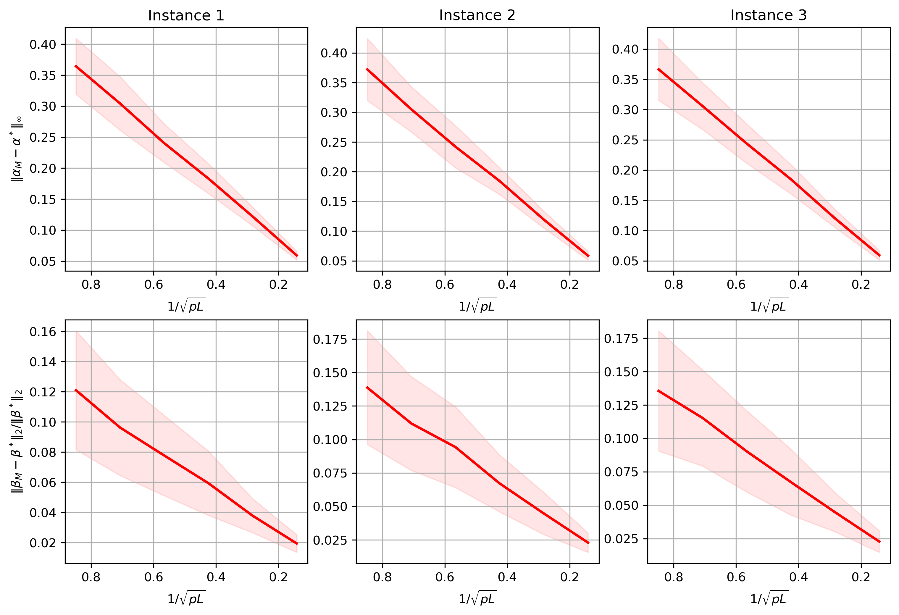
To validate the statistical rates in Theorem 2, we use the above method to generate the covariates and three times. This gives us three different instances of the covariates and the parameter . For each given instance, we consider different pairs, which are listed below.
| 1 | 0.5 | 0.222 | 0.625 | 0.4 | 0.278 | |
| 50 | 25 | 25 | 5 | 5 | 5 |
For each pair, comparion graph , is generated and the MLE is calculated based on the available data. This process is repeated times, and the averaged and , as well as their associated standard deviations, are recorded. The results are depicted in Figure 1 for each of the three instances. Note that and are nearly proportional to , lending further support of the results in Theorem 2. The results are insensitive to three different instances, as expected.
5.2 Distributional Results
We employ the same method given in §5.1 to generate the covariates and once and fix them throughout the simulation. Letting the effective sample size (here and ), we choose the pairs with or and . For each pair, the graph and data are generated times and the MLEs for all simulations are recorded. Figure 2 presents the Q-Q plots for checking the normality of , the first component of . The results show that follows closely the normal distribution.

In addition to checking the asymptotic normality, we now verify the asymptotic variance of our estimator. As an illustration, we consider the linear combination , where and is the -th vector from the standard basis of . Based on 250 simulations with and , the histograms of the following two standardized random variables are plotted:
| (11) |
This uses the asymptotic theory with plug-in asymptotic variance using the true and estimated parameters, where is the projection of onto linear space . Figure 3 shows that the histograms closely follow the standard Gaussian density. The first row of Figure 3 is presented in the regime with . It holds that, even when the sample size is very small, the two density plots are still very close to the standard Gaussian density. The second row of Figure 3 is drawn based on the setting where . In this case, the density plots of and are more stable and close to the standard Gaussian curve. These results, in turn, support our theoretical results in Theorem 8.

5.3 Comparison with BTL Model Without Covariates
In this section, we conduct a series of simulations to compare the results with the model without using covariates in terms of the proportion of information being explained, prediction accuracy, and sensitivity analysis.
- •
We show the first merit of our proposed method, in terms of the proportion of information being explained.
We record the following quantity , which quantifies the proportion of information being explained by the covariates. We consider the same pair presented in Section 5.1. For each pair, we generate the comparison graph , the comparison results and solve the MLE for times. We report the mean and standard deviation of the concerned quantity for each pair based on these repetitions. The results are presented in the following Table 1.
Table 1: Mean and standard deviation of for each pair based on repetitions. We conclude from Table 1, involving the covariates helps reduce the magnitude of unexplained information for all settings. Therefore, this further helps in making out-of-sample predictions, and we will discuss this point in the following step.
- •
Second, we present the prediction performance of our model and compare it with BTL model without covariates. We generate a new set of covariates where falls in the same column space of . With these new covariates, for any , the out-of-sample probability becomes
Using the covariate information, the probability predicted by our model is
However, when one does not take the covariates information into consideration, the best one can do is to use the estimated score under the original BTL model, as Chen et al. 2019; Gao et al. 2021 did. In this case, the predicted probability is
In Table 2 we present the mean square error and for the six pairs we mentioned above. The results show the mean and standard deviation of the mean square error calculated over repetitions. As we can see from Table 2, the estimator , which takes the covariate information into consideration, performs much better than the one without covariate information.
With covariates Without covariates Table 2: Mean and standard deviation of mean square error and under each setting based on simulations. - •
Lastly, we test the sensitivity of our model by violating the linearity assumption of our model. And subsequently, we also compare its performance to that of the BTL model without covariates.
We modify the underlying model to be
where when we fit the model and when we make prediction. Here is a nonlinear function. In our experiment, we fix and let
(12) and is chosen to be and to accommodate different levels of non-linearity. With covariate information, the winning probability is still predicted as
while the predicted probability of the original BTL model is
In Tables 3 and 4 we present the results when is chosen to be and . We again consider the mean square error and as the metric. The experiments are repeated times for each pair and we report the mean and standard deviation.
With covariates Without covariates Table 3: Mean and standard deviation of mean square error and under each setting based on simulations. The level of non-linearity in (12) is chosen to be . With covariates Without covariates Table 4: Mean and standard deviation of mean square error and under each setting based on simulations. The level of non-linearity in (12) is chosen to be . From Table 3 and 4 we can see that our model consistently performs better than the original BTL model when different levels of non-linearity exist.
5.4 Application to Pokemon Challenge Dataset
We apply the proposed method to study the Pokemon Challenge Dataset. The original dataset can be found at https://www.kaggle.com/c/intelygenz-pokemon-challenge/data. This dataset records the pairwise competition records among 800 Pokemon, whose covariate information is also recorded. This dataset contains competition results, each competition takes place between two pokemons and has one winner.
Our experiments mainly focus on predicting the ability of the mega evolved pokemons. We think that a mega evolved pokemon has the same intrinsic ability (same ) as pre-evolutionary pokemon, and the mega evolution may only change the covariates . We have mega evolved pokemons in this dataset, and we randomly select of them to test our predictive performance. Among these remaining pokemons for training purposes, we select the largest connected component of their comparison graph. Eventually we have pokemons left for training. For each pokemon, we select , , Mega or not as their covariates. Here Attack and HP denote the ability to attack and durability, respectively. The variable Mega or not takes binary value and represents whether this pokemon is mega evolved or not. We optimize the likelihood of our CARE model in (4) using training data and record and .
We first investigate the statistical significance of these 3 variables we are interested in. This amounts to testing the following hypothesis testing problems for each feature:
The test statistics are given by for all and the corresponding p-values are calculated via the asymptotic normality results in §4. The results are depicted in Table 5, and these three variables are all statistically significant.
| Estimate | p-value | |
| Attack | ||
| HP | ||
| Mega or not |
We then evaluate the competitions performance of the mega evolved pokemons in the test sample, whose pre-evolutionary versions are the training data. We predict the score of an evolved pokemon as where is the estimated intrinsic score of the pre-evolutionary version and is the new covariates of this mega evolved pokemon. Here we apply a soft-thresholding to the part with and for each pokemon in the training dataset. This corresponds to set those estimates that are statistically indifferent from zero to zero. The use of significant level is to control the familywise false positive rates at a level of .
In order to formalize the metric we used to test our procedure, we introduce the following notation first. Let be set of the pokemons we want to predict and let be set of the pokemons in the training data who have competitions with pokemons in . Given any two pokemons and , we let be the competitions between and and define . For each pokemon from , we further define the estimated score as . We use the following quantities and as measures of the prediction loss for pokemons in when we have covariate information
As a comparison, for the original BTL model, we let be the estimated score under the original BTL model. Since there no covariate information is involved, for pokemons from , their are set to be the estimated scores of their pre-evolutionary versions. In addition, for pokemons from , their scores are set to be estimated via the training data. The loss for our method and original BTL model are reported in Table 6. As we can see, our model achieves a significant improvement over the original BTL model.
| Loss | With covariates | Without covariates |
| MSE | ||
| Logistic |
6 Conclusion and Discussion
In this paper, we study a Covariate-Assisted Ranking Estimation (CARE) model systematically. This allows us to incorporate the covariate information of compared items into the ranking framework, which includes the standard BTL model as a particular case. We derive the minimal sample complexity required for statistical consistency and uncertainty quantification for MLE based on novel proof techniques and illustrate the theory and methods using the mutual fund holding dataset. The empirical results lend further support to the CARE model over the classical BTL model.
There are a few future directions worth exploring. First, it is worth extending the idea of incorporating covariates into a more general ranking framework, such as the Plackett-Luce or nonparametric models, under a more general comparison graph. In contrast, our work only studies the BTL model with the Erdős-Rényi comparison graph. Second, it would be interesting if some structure assumptions exist on the parameters and , such as sparsity. In this scenario, one shall leverage certain regularizers on and in the likelihood function to achieve a solution that generalizes well. Third, except for the covariate, one may also incorporate time information into the ranking framework as in many real applications, the underlying scores of compared items change over time. Lastly, in our paper, we consider the scenario where the underlying score of the -th item is given by in the sense that the overall score of the -th item is the summation of its intrinsic score and its covariate times one specific evaluation criterion . It would be interesting if we do a ranking based on data evaluated from multiple sources. In specific, suppose that we have users and items and the score of the -th item, evaluated by the -th person, is . It would be interesting to derive novel statistical estimation and uncertainty quantification principles for ranking models under this setting. We will leave these open problems for future research.
acknowledgments-disclosure-of-funding.
Research supported by the NSF grants DMS-2052926, DMS-2053832, DMS-2210833, and ONR N00014-22-1-2340.Supplementary materials to “Uncertainty Quantification of MLE for Entity Ranking with Covariates”
Appendix A Proof Outline of Estimation Results
In this section, we first present the proof outline for Theorem 2. The detailed proof of Theorem 2 is presented in §A.5.
To understand statistical error of , we begin with analyzing the regularized MLE
| (13) |
where for and then make connections with by a properly chosen . The introduction of - regularization as a intermediate step is essential for ensuring the MLE fall in a bounded area around the ground truth through this regularized MLE. Therefore, strong convexity of the loss holds in this bounded area. Prevailing methodologies for examining the BTL model (Chen et al. 2019 and Chen et al. 2022b) also relies on this regularization to ensure strong convexity of the loss.
Before proceeding, we introduce the following two quantities and indicating the difficulty of recovering
The regularized MLE solves a strong convex problem whose estimation error bounds are derived in Theorem 11 below.
Theorem 11.
Suppose for some and . We consider for any absolute constants and
for some . Let be the solution of the regularized MLE Eq. (13). Then with probability at least , we have
where .
Theorem 11 presents the statistical rates of the regularized MLE in (13). Before presenting the formal proof for Theorem 11, in the following several subsections A.1, A.2 and A.3 , we focus on establishing its associated building blocks.
Given that our final objective is to establish the statistical rates of the Maximum Likelihood Estimator (MLE) applied to the unregularized loss function (3), we present a formal proof of Theorem 2 in §A.5, leveraging the insights provided by Theorem 11.
A.1 Preliminaries and Basic Results
In this subsection, we study the theoretical properties of the gradient and Hessian of the loss function in (13). Their expressions are given by
| (14) | ||||
| (15) |
The gradient of at is controlled by the following lemma.
Lemma 12.
With given by Theorem 11, the following event
happens with probability exceeding for some which only depend on .
Next, we proceed to analyzing the Hessian matrix . First, we consider and study its eigenvalues in Lemma 13.
Lemma 13.
Suppose for some . The following event
happens with probability exceeding when is large enough.
Proof.
See §C.3 for a detailed proof. ∎
In the rest of the content, without loss of generality, we assume the conditions stated in Lemma 13 hold. Moreover, with the help of Lemma 13, we next analyze the Hessian and summarize its theoretical properties in Lemma 14 and Lemma 15, respectively.
Lemma 14.
Suppose event holds, we obtain
Proof.
Since , we have
∎
Lemma 15.
Suppose event happens. Then for all such that , , we have
where .
A.2 Convergence of Projected Gradient Descent
In this subsection, we consider a sequence of iterates which is generated by the following projected gradient descent algorithm with stepsize and the number of iterations .
We initialize at and the target loss given in (13) is strongly convex. The projected gradient descent is employed (since the likelihood has a linear constraint) to ensure the iterates converge to the -regularized MLE exponentially. In the following section, using the leave-one-out analysis, we also show at the same time stays close to for all . Therefore, combine these two parts together, we are able to conclude that is also close to .
We summarize the theoretical findings in the following Lemma 16, Lemma 17 and Lemma 18, respectively.
Lemma 16.
Under event , we have
where .
Next, we prove that the initial point is not far from .
Lemma 17.
On the event happens, it follows that
Proof.
See §C.6 for a detailed proof. ∎
Lemma 18.
On event , there exists some constant such that
Proof.
See §C.7 for a detailed proof. ∎
In this subsection, we prove that the iterate converges to geometrically and enjoys a good optimization error after iterations. In order to prove the distance between and , i.e. the statistical error of , in the next subsection, we leverage the leave-one-out technique and use induction to prove that the iterate stays close to our initial point , even after iterations.
A.3 Analysis of Leave-one-out Sequences
In this section, we construct the leave-one-out sequences (Ma et al. 2018; Chen et al. 2019; Chen et al. 2020) and bound the statistical error by induction. To construct the leave-one-out sequence, we consider the following loss function for any .
Then for any , we construct the leave-one-out sequence in the way of Algorithm 2.
With the help of the leave-one-out sequences, we do induction to demonstrate that the iterate will not be far away from when In specific, we take again and . With the leave-one-out sequences in hand, we prove the following bounds by induction for .
| (A) | ||||
| (B) | ||||
| (C) | ||||
| (D) |
For , since , the (A) (D) hold automatically. In the following lemmas, we prove the conclusions of (A)-(D) for the -th iteration are true when the results hold for the -th iteration.
Lemma 19.
Proof.
See §C.8 for a detailed proof. ∎
Lemma 20.
Proof.
See §C.9 for a detailed proof. ∎
Lemma 21.
Proof.
See §C.10 for a detailed proof. ∎
Lemma 22.
Proof.
See §C.11 for a detailed proof. ∎
A.4 Proof of Theorem 11
In this subsection, we aim at providing proof for Theorem 11 by combining the results established above.
For any , by Taylor expansion, one obtains
where is some real number between and . As a result, it holds that
By the Cauchy-Schwartz inequality, we have
where and is large enough. The last inequlity holds from the results derived in §A.2 and §A.3. Then for and such that , we have
Similarly, we also obtain
A.5 Proof of Theorem 2
With all necessary building blocks at hand, in this subsection, we provide the formal proof for Theorem 2. In specific, we assume in the following proof and it is easy to extend the proof to the regime . The way to solve this is changing the power in Lemma 12 and Lemma 13 to a larger number.
Proof.
Consider the following MLE
| (16) |
We choose in the definition of such that
for some . As long as for some absolute constants , the proof of Lemma 18 is still valid and Theorem 11 still holds for this . For large enough such that satisfies the constraints in Eq. (16), by the optimality of we know that . On the other hand, by Taylor’s expansion
where for some .
This leads to
| (17) |
Next, we first define the norm as
Therefore, we have
as long as
As a result, by Lemma 15 we have
| (18) |
Combine Eq. (17) and Eq. (18) we have
Therefore, after some simple calculations, it holds that
And, when is large enough, we have
| (19) | ||||
| (20) |
where and . As a result, falls in the interior of the inequality constraints in Eq. (16). By the convexity of and its strong convexity in , we have . Therefore, by Eq. (19) and Eq. (20) we have
| (21) | ||||
| (22) |
The result of and hold based on the same derivations in Section A.4 and we omit the corresponding details. ∎
Appendix B Proof of Inference Results in Section 4
In this section we first introduce our extension to top-K testing and provide the proof outlines for Theorem 5. Then, we prove Theorem 8 and Corollaries 9 and 10, based on the results of Theorem 5. The details of proofs in this section is deferred to Section C. We next introduce some building blocks for the proof of main theorems.
B.1 Extension to Top-K set hypothesis testing
In this section, we extend the method to conduct the top-K test using estimators for overall scores (for simplicity, here we define the overall scores as and its estimators as ).
We use the following statistics to construct top-K test simultaneously for all elements in
It’s distribution can be approximated by the bootstrap counterpart
We are able to achieve similar theoretical results by following the similar proof procedure of Theorem 5 in Fan et al. 2023 for and . Let be the -th quantile of , we have the following theorem for the test statistics .
Theorem 23.
Under the conditions of Theorem 1, we have
Next, we introduce some applications on constructing (simultaneous) one-sided confidence intervals for out-of-sample ranks via the distribution of in the following two examples.
Example 24.
For an item of interest, and let be the targeted rank threshold, we are interested in the following testing problem
| (23) |
Let be the estimated -th quantile of from the bootstrap samples. As a result, we have
Similarly, this implies
This yields a critical region at a significance level of for the test (23)
B.2 Proof Outline
Lemma 25.
For , with probability at least we have
- •
;
- •
, , .
- •
, for any .
Proof.
See §D.1 for a detailed proof. ∎
Recall that we define the norm as
Then for any and , we have .
B.3 Proof Outline of Theorem 5
In this subsection, we provide the proof outline for Theorem 5. The following lemma gives a bound for , which validates the first part of Theorem 5.
Theorem 26.
Under the assumptions of Theorem 2, with probability at least we have
Proof.
See §D.2 for a detailed proof. ∎
Next, we consider controlling the magnitude of for in order to prove the second part of Theorem 5.
Recall that we define the quadratic approximation to in (6), which is also given as below:
We adopt the following notation for a given vector ,
which acts as a marginal likelihood function for the -th coordinate given the other coordinates fixed. Accroding to this definition, we have the following proposition. The proof of Proposition 27 is included in §D.3.
Proposition 27.
For , is the minimizer of the univariate function .
By changing the coordinates that we fix, we define as the minimizer of . Here we fix and optimize based on this fixed parameter. Explicitly, the minimizer is calculated as
In order to bound we bound and separately.
In terms of , we provide an upper bound for this quantity in Lemma 28.
Lemma 28.
Under the assumptions of Theorem 2, as long as , for , with probability at least we have
On the other hand, for a given we let
| (24) |
Here we consider the marginal loss of in the -th coordinate given other coordinates fixed. Similar to Proposition 27, we have the following proposition for . The proof of Proposition 29 is also included in §D.3.
Proposition 29.
For , is the minimizer of the univariate function .
We now describe the intuition of bounding . Since is the minimizer of and is the minimizer of . Therefore, as long as and are close enough, the difference between their minimizers and is small. We summarize this finding in the following lemma 30.
Lemma 30.
Under the assumptions of Theorem 2, for , with probability at least we have
Theorem 31.
Under the assumptions of Theorem 2, as long as and for some fixed constant , with probability at least , for we have
If we further assume , then with probability at least , for we have
B.4 Proof of Theorem 5
Proof of Theorem 5.
B.5 Proof of Theorem 8
This subsection aims at deriving theoretical proof for Theorem 8.
Proof.
The following content is conditioned on the event . Recall that is the projection of onto linear space . Therefore, we obtain
By Proposition 34 we have . Since , we also have . Let . Then we have
As a result, we have
For such that and , we define
Then we have
with probability exceeding (randomness comes from ). As a result, by Berry 1941 we have
with probability exceeding (randomness comes from ). And, we know that and
with probability exceeding . Therefore,
with probability exceeding (randomness comes from ). On the other hand, by Theorem 5 we have
with probability at least . Therefore, we conclude the first part of Theorem 8.
We next take all randomness into consideration. For simplicity we denote by
To begin with, for fixed we have
As a result, we have
| (25) |
Consider event , where is some constant such that . Then we consider the following three events
Then we have
| (26) | ||||
| (27) |
On the other hand, for we have
As a result, we know that
| (28) |
By Eq. (25) we have
On the other hand, we have
Therefore, we have
| (29) |
For we also have
| (30) |
By definition we have
By Eq. (25) we have
On the other hand, we have
Therefore, we have
| (31) |
Combine Eq. (27), Eq. (28) and Eq. (30) we know that
Therefore, by Eq. (29), Eq. (31) we have
Since the above inequality holds for every , we prove the desired result.
Thus, we finally conclude our proof of Theorem 8.
∎
B.6 Proof of Corollary 9
Proof of Corollary 9.
Let be canonical basis vectors of . By taking for in Theorem 8, we only have to show that , and this is also equivalent to . By the definition of we have
As a result, the first part of Corollary 9 is proved by Theorem 8.
For simplicity we denote by . To begin with, for fixed we have
As a result, we have
| (32) |
Consider event , where is some constant such that . Then we consider the following three events
Then we have
| (33) | ||||
| (34) |
On the other hand, for we have
As a result, we know that
| (35) |
By Eq. (32) we have
On the other hand, we have
Therefore, we have
| (36) |
For we also have
| (37) |
By definition we have
By Eq. (32) we have
On the other hand, we have
Therefore, we have
| (38) |
Combine Eq. (34), Eq. (35) and Eq. (37) we know that
Therefore, by Eq. (36), Eq. (38) we have
Since the above inequality holds for every , we prove the desired result.
∎
B.7 Proof of Corollary 10
The proof of Corollary 10 except the refined bound Eq. (10) follows directly from the proof of Theorem 8. Therefore, we omit the details and only prove Eq. (10) here. We prove the following lemma first.
Lemma 32.
Consider some fixed constants for , and random variable
| (39) |
Conditioned on the comparison graph , with probability exceeding we have
Proof.
Let . Then we know that and . As a result, by Hoeffding inequality, with probability at least , we have
| (40) |
On the other hand, since are independent random variables, we know that
As a result, we have . Therefore, by Eq. (40) we know that
with probability exceeding . ∎
Proof of Eq. (10).
Conditioned on the comparison graph , the entries of can be written as the form Eq. (39). By Lemma 32 and union bound, conditioned on the comparison graph , we know that
| (41) |
with probability at least . By Proposition 34 we know that
By the definition of we know that
under event . As a result, we have
| (42) | ||||
| (43) |
with probability at least . Combine Eq. (41) and Eq. (43) we know that
with probability at least . On the other hand, by Theorem 5, we have
with probability at least . We know that
with probability at least . ∎
Appendix C Proof of Auxiliary Lemmas in Section A
In this section, we prove detailed proof of aforementioned building blocks.
C.1 Proof of Proposition 1
Proof.
Assume that there are two parameter vectors and such that
Since , we know that
Let and be a -dimensional vertoc whose entries are all one, then we know that
Since , we know that
This implies . Therefore, we have . This is equivalent to
Since has full column rank, we know that . As a result, we must have .
∎
C.2 Proof of Lemma 12 and Its Corollary
In this subsection, we provide the proof of Lemma 12 in the sense that we provide an upper bound for the gradient vector in -norm.
Proof.
The gradient is calculated as
Since , we have
| and |
as long as is large enough. Thus, with high probability (with respect to the randomness of ), we have
and
Let and . By matrix Bernstein inequality (Tropp 2015), we have
with probability exceeding as long as and . On the other hand, we have
To summarize, we have
with probability exceeding . ∎
Once Lemma 12 is established, we have the following lemma which can be viewed as a direct corollary of Lemma 12.
Lemma 33.
With given by Theorem 11, the following event
is contained by the event . As a result, happens with probability exceeding .
Proof.
By the fundamental theorem of calculus we know that
where . So for all such that , we have
Under event , we have
And, under event , we have . As a result, is contained by . ∎
C.3 Proof of Lemma 13
Proof.
Let be any matrix with orthonormal rows such that the row space of is , where is the dimension of . Then, it holds that
Let for . Then we have and
as long as is large enough. Furthermore,
By the matrix Chernoff inequality (Tropp 2012), we have
As a result, if for some , we have
This concludes the proof of Lemma 13. ∎
C.4 Proof of Lemma 15
In this subsection, we provide the proof of Lemma 15 by providing a lower bound for
Proof.
For pair , without loss of generality we assume , we then obtain
One the other hand, it holds that
Therefore, we obtain
where . As a result, for the Hessian we have
This completes the proof of Lemma 15. ∎
C.5 Proof of Lemma 16
Proof.
Since is -strongly convex and -smooth on the event , we know that
As a result, when event happens, we have
Therefore, under event , we have
∎
C.6 Proof of Lemma 17
In this section, we prove is not far from the initial point .
Proof.
Since is the minimizer, we have that . By the mean value theorem, for some between and , we have
As a result, we have
Therefore, we get
As a result, on event we have
We conclude the proof of Lemma 17. ∎
C.7 Proof of Lemma 18
C.8 Proof of Lemma 19
Proof.
By definition we know that
Consider . By the fundamental theorem of calculus we have
Let be large enough such that
In addition, by the assumption of induction, we have
Then by Lemma 15, we have
On the other hand, by Lemma 14, we have
Let , then we have
Since , it holds that
Therefore, on the event , we have
as long as . ∎
C.9 Proof of Lemma 20
Proof.
For any , by definition we have
We consider . By the fundamental theorem of calculus we have
| (44) | ||||
| (45) | ||||
| (46) |
Consider which is large enough such that
Then we also have
Use the same approach derived in §C.8, we have
| (47) |
as long as .
On the other hand, since , it remains to bound By definition, we have
By definition, we also have
Consider random variable . By Chernoff bound (Tropp 2012), we know that
as long as for some . As long as , we have for . Since , by Hoeffding’s inequality and union bound, we get
with probability exceeding conditioning on as long as . On the other hand, since with probability exceeding , we have
with probability exceeding .
On the other hand, for we have
where
Consider . Since , we have that
By Bernstein inequality we know that
As a result, for we have
In summary, there exists constants which are independent of such that
| (48) |
with probability exceeding . Combining Eq. (46), Eq. (47) and Eq. (48) we have
as long as and is large enough such that .
∎
C.10 Proof of Lemma 21
Proof.
For , we have
For , we have
By Lemma 33, with probability at least we have
as long as
In this case, for we have
| (49) |
On the other hand, for we have
| (50) | ||||
| (51) |
Normalizing the numerators below to 1 and by the mean value theorem, there exists some between and such that
| (52) |
Combining Eq. (51) and Eq. (52), we have
By taking absolute value on both side, we get
Since , we have
By the defintion of we have
Consider which is large enough such that
Then we have
Then it holds that,
Using for , we have
Combine this result with Eq. (49), we get
as long as , and . This concludes our proof for Lemma 21. ∎
C.11 Proof of Lemma 22
Proof.
For any , we have
As a result, we have
as long as . ∎
Appendix D Proof of Auxiliary Lemmas in Section B
D.1 Proof of Lemma 25 and Two Propositions (Propositions 34 and 35)
Proof of Lemma 25.
(1) By definition for we have
Since , by Bernstein inequality we have
with probability exceeding , as long as . On the other hand, since , we know that . As a result, we have
(2) By definition we have
with probability at least . Similarly, we have
and
with probability at least .
(3) For , by definition we know that is the average of independent Bernoulli random variables. By Hoeffding’s inequality we know that
with probability at least . As a result, by union bound we know that
holds for all with probability at least . ∎
We also include here two propositions which are also involved in the later proofs.
Proposition 34.
is the solution of the following linear equations
Proposition 35.
Under event , we have
We next provide the proof of Proposition 35 here.
Proof of Proposition 35.
Since , by taking variance (conditioned on ) on the both sides we have
| (53) |
On the other hand, by considering the covariance (conditioned on ) of and we get
As a result, we know that
| (54) |
Combine Eq. (53) and Eq. (54) we get
| (55) |
By taking variance on the both sides of , we have . This also implies . As a result, Eq. (55) can be also written as
This immediately implies . Under event , we have . As a result, for any , we have
As a result, we have for all . Combine this fact with , we know that
∎
D.2 Proof of Theorem 26
Proof.
We know that
Let
we have
| (56) |
On the other hand, we know that
| (57) |
Combine Eq. (56) and Eq. (57) we have
| (58) |
For we have
By definition we have
By Lemma 13 we know that
holds uniformly for all with probability at least . As a result, we get
| (59) |
with probability exceeding . Since , we know that
As a result, we get
| (60) |
By Lemma 15 we know that
| (61) |
with probability exceeding . Therefore, combine Eq. (59), Eq. (60) and Eq. (61) we get
with probability exceeding . ∎
D.3 Proof of Proposition 27 and Proposition 29
We denote by . By the definition of and we know that for any and , we have
On the other hand, under Assumption 3 we have the following lemma.
Lemma 36.
For any , there exists a such that .
Proof.
We only have to show that for any , . Assume there exists a such that . First of all, we must have . Since , we must have as . Since , we know that there exists a non-zero vector such that . By the definition of , we know that . Recall the definition of and Assumption 3 in §3. Since , we know that , so we must have . As a result, this contradicts to Assumption 3 since . ∎
Proof of Proposition 27 and 29.
Assume there exists a such that . Then we let be the vector such that and . And, let be the vector in such that . Then we have
This contradicts to the definition of Eq. (5).
Similarly, if we assume that there exists a such that . Then we let be the vector such that and . And, let be the vector in such that . Then we have
This contradicts to the definition of Eq. (3). ∎
D.4 Auxiliary Results for Proving Lemma 28
In this section we include two results which are helpful to the proof of Lemma 28 in §D.5. These two results are analogies of Theorem 2 and Theorem 26 which we have proven before. The main difference is we replace with . As a result, the following two results can be viewed as the leave-one-out version of Theorem 2 and Theorem 26. To be more specific, we define as
and let be the solution of the following equations
Lemma 37.
Suppose for some and . We consider for any absolute constants . Then for every and , with probability at least we have
Lemma 38.
Under the assumptions of Theorem 37, for every , with probability at least we have
D.5 Proof of Lemma 28
Proof.
Next, we bound - one by one. Before proceeding, the denominator can be bounded as
with probability at least .
For , by Lemma 37 we have
So the numerator of can be bounded as
with probability at least . As a result, can be bounded as
| (63) |
with probability at least .
When it comes to , by definition we know that is independent with for all . As a result, by Bernstein’s inequality and Lemma 38 we know that
| (64) | ||||
| (65) | ||||
| (66) | ||||
| (67) |
with probability at least . On the other hand, by Lemma 38 we have
| (68) | ||||
| (69) | ||||
| (70) |
and
| (71) |
with probability exceeding . Combine Eq. (67), Eq. (70) and Eq. (71) we finally bound the numerator of as
with probability at least . As a result, we have
| (72) |
with probability at least .
We finally consider bounding . By definition, we know that
Combine the two equations we get
| (73) |
For , it is easy to see . By definition we have
For , by Hoeffding inequality, we have
conditioned on with probability at least . On the other hand, since with probability at least , we have
with probability at least . Furthermore, by Lemma 25 we have
with probability at least . For , we have
with probability at least . Therefore, for we have
| (74) | ||||
| (75) |
with probability exceeding .
For , since , it holds that
As a result, it follows that
with probability exceeding . On the other hand, we obtain
with probability at least . That is to say, we have
| (76) |
with probability at least .
Combine Eq. (75) and Eq. (76) with Eq. (73), we know that
with probability at least . Since , we have
As a result, we know that
| (77) |
with probability at least . Therefore, for we finally achieve
| (78) | ||||
| (79) |
with probability at least .
And, by Eq. (77) we know that
with probability exceeding . Combine with Eq. (72) we have
| (80) |
with probability exceeding . Combine Eq. (63), Eq. (80) and Eq. (79) we know that
with probability at least .
∎
D.6 Proof of Lemma 30
Proof.
Since is the minimizer of , we know that . By the mean value theorem we know that
where is some real number between and . As a result, we have
By the definition Eq. (4) and Eq. (24), we have
We first estimate the difference . We have
with probability at least . On the other hand, we have
| (81) | ||||
| (82) | ||||
| (83) | ||||
| (84) | ||||
| (85) | ||||
| (86) |
where
By Taylor expansion we know that
where is some real number between and . As a result, we have
| (87) |
Combine Eq. (86) and Eq. (87) we have
with probability exceeding . As a result, we have
where
and
with probability exceeding . On the other hand, we know that
with probability at least . To sum up, we have
with probability at least . ∎
Appendix E Details of Real Data Experiments
In this section, we provide the details in computing the maximum likelihood estimator . We first generated the variables and comparisons as described in §5.4. We standardized each column to make sure they have mean and standard deviation and then multiplied by (scale to the order of as mentioned in the main text). In real-world data the numbers of comparisons between each compared pair are not the same, so we denote by the number of comparisons between pair . Let be all the comparisons we have, then the negative log-likelihood can be written as
References
- Baltrunas et al. (2010) L. Baltrunas, T. Makcinskas, and F. Ricci. Group recommendations with rank aggregation and collaborative filtering. In Proceedings of the fourth ACM conference on Recommender systems, pages 119–126, 2010.
- Banerjee (1973) K. Banerjee. Generalized inverse of matrices and its applications, 1973.
- Berry (1941) A. C. Berry. The accuracy of the gaussian approximation to the sum of independent variates. Transactions of the american mathematical society, 49(1):122–136, 1941.
- Bradley and Terry (1952) R. A. Bradley and M. E. Terry. Rank analysis of incomplete block designs: I. the method of paired comparisons. Biometrika, 39(3/4):324–345, 1952.
- Chau et al. (2023) S. L. Chau, M. Cucuringu, and D. Sejdinovic. Spectral ranking with covariates. In Machine Learning and Knowledge Discovery in Databases: European Conference, ECML PKDD 2022, Grenoble, France, September 19–23, 2022, Proceedings, Part V, pages 70–86. Springer, 2023.
- Chen et al. (2022a) P. Chen, C. Gao, and A. Y. Zhang. Optimal full ranking from pairwise comparisons. The Annals of Statistics, 50(3):1775–1805, 2022a.
- Chen et al. (2022b) P. Chen, C. Gao, and A. Y. Zhang. Partial recovery for top-k ranking: Optimality of mle and suboptimality of the spectral method. The Annals of Statistics, 50(3):1618–1652, 2022b.
- Chen et al. (2017) X. Chen, S. Gopi, J. Mao, and J. Schneider. Competitive analysis of the top-k ranking problem. In Proceedings of the Twenty-Eighth Annual ACM-SIAM Symposium on Discrete Algorithms, pages 1245–1264. SIAM, 2017.
- Chen and Suh (2015) Y. Chen and C. Suh. Spectral mle: Top-k rank aggregation from pairwise comparisons. In International Conference on Machine Learning, pages 371–380. PMLR, 2015.
- Chen et al. (2019) Y. Chen, J. Fan, C. Ma, and K. Wang. Spectral method and regularized mle are both optimal for top-k ranking. Annals of statistics, 47(4):2204, 2019.
- Chen et al. (2020) Y. Chen, Y. Chi, J. Fan, C. Ma, and Y. Yan. Noisy matrix completion: Understanding statistical guarantees for convex relaxation via nonconvex optimization. SIAM journal on optimization, 30(4):3098–3121, 2020.
- Chen et al. (2021) Y. Chen, Y. Chi, J. Fan, C. Ma, et al. Spectral methods for data science: A statistical perspective. Foundations and Trends® in Machine Learning, 14(5):566–806, 2021.
- Cheng et al. (2010) W. Cheng, K. Dembczynski, and E. Hüllermeier. Label ranking methods based on the plackett-luce model. In ICML, 2010.
- Dwork et al. (2001) C. Dwork, R. Kumar, M. Naor, and D. Sivakumar. Rank aggregation methods for the web. In Proceedings of the 10th international conference on World Wide Web, pages 613–622, 2001.
- Erdos et al. (1960) P. Erdos, A. Rényi, et al. On the evolution of random graphs. Publ. Math. Inst. Hung. Acad. Sci, 5(1):17–60, 1960.
- Esseen (1942) C.-G. Esseen. On the liapunov limit error in the theory of probability. Ark. Mat. Astr. Fys., 28:1–19, 1942.
- Fan et al. (2023) J. Fan, Z. Lou, W. Wang, and M. Yu. Spectral ranking inferences based on general multiway comparisons. arXiv preprint arXiv:2308.02918, 2023.
- Fan et al. (2024+) J. Fan, Z. Lou, W. Wang, and M. Yu. Ranking inferences based on the top choice of multiway comparisons. Journal of American Statistical Association, 2024+.
- Finch (2022) H. Finch. An introduction to the analysis of ranked response data. Practical Assessment, Research, and Evaluation, 27(1):7, 2022.
- Gao et al. (2021) C. Gao, Y. Shen, and A. Y. Zhang. Uncertainty quantification in the bradley-terry-luce model. arXiv preprint arXiv:2110.03874, 2021.
- Guiver and Snelson (2009) J. Guiver and E. Snelson. Bayesian inference for plackett-luce ranking models. In proceedings of the 26th annual international conference on machine learning, pages 377–384, 2009.
- Guo et al. (2018) Y. Guo, P. Tian, J. Kalpathy-Cramer, S. Ostmo, J. P. Campbell, M. F. Chiang, D. Erdogmus, J. G. Dy, and S. Ioannidis. Experimental design under the bradley-terry model. In IJCAI, pages 2198–2204, 2018.
- Hajek et al. (2014) B. Hajek, S. Oh, and J. Xu. Minimax-optimal inference from partial rankings. Advances in Neural Information Processing Systems, 27, 2014.
- Han et al. (2020) R. Han, R. Ye, C. Tan, and K. Chen. Asymptotic theory of sparse bradley–terry model. The Annals of Applied Probability, 30(5):2491–2515, 2020.
- Harper and Konstan (2015) F. M. Harper and J. A. Konstan. The movielens datasets: History and context. Acm transactions on interactive intelligent systems (tiis), 5(4):1–19, 2015.
- Hunter (2004) D. R. Hunter. Mm algorithms for generalized bradley-terry models. The annals of statistics, 32(1):384–406, 2004.
- Jang et al. (2016) M. Jang, S. Kim, C. Suh, and S. Oh. Top- ranking from pairwise comparisons: When spectral ranking is optimal. arXiv preprint arXiv:1603.04153, 2016.
- Jang et al. (2018) M. Jang, S. Kim, and C. Suh. Top- rank aggregation from -wise comparisons. IEEE Journal of Selected Topics in Signal Processing, 12(5):989–1004, 2018.
- Jin et al. (2020) T. Jin, P. Xu, Q. Gu, and F. Farnoud. Rank aggregation via heterogeneous thurstone preference models. In Proceedings of the AAAI Conference on Artificial Intelligence, volume 34, pages 4353–4360, 2020.
- Li et al. (2019) H. Li, D. Simchi-Levi, M. X. Wu, and W. Zhu. Estimating and exploiting the impact of photo layout: A structural approach. Available at SSRN 3470877, 2019.
- Li et al. (2022) X. Li, D. Yi, and J. S. Liu. Bayesian analysis of rank data with covariates and heterogeneous rankers. Statistical Science, 37(1):1–23, 2022.
- Liu et al. (2022) Y. Liu, E. X. Fang, and J. Lu. Lagrangian inference for ranking problems. Operations Research, 2022.
- Luce (2012) R. D. Luce. Individual choice behavior: A theoretical analysis. Courier Corporation, 2012.
- Ma et al. (2018) C. Ma, K. Wang, Y. Chi, and Y. Chen. Implicit regularization in nonconvex statistical estimation: Gradient descent converges linearly for phase retrieval and matrix completion. In International Conference on Machine Learning, pages 3345–3354. PMLR, 2018.
- Massey (1997) K. Massey. Statistical models applied to the rating of sports teams. Bluefield College, 1997.
- Maystre and Grossglauser (2015) L. Maystre and M. Grossglauser. Fast and accurate inference of plackett–luce models. Advances in neural information processing systems, 28, 2015.
- Negahban et al. (2012) S. Negahban, S. Oh, and D. Shah. Iterative ranking from pair-wise comparisons. Advances in neural information processing systems, 25, 2012.
- Pananjady et al. (2017) A. Pananjady, C. Mao, V. Muthukumar, M. J. Wainwright, and T. A. Courtade. Worst-case vs average-case design for estimation from fixed pairwise comparisons. arXiv preprint arXiv:1707.06217, 2017.
- Plackett (1975) R. L. Plackett. The analysis of permutations. Journal of the Royal Statistical Society: Series C (Applied Statistics), 24(2):193–202, 1975.
- Richardson et al. (2006) M. Richardson, A. Prakash, and E. Brill. Beyond pagerank: machine learning for static ranking. In Proceedings of the 15th international conference on World Wide Web, pages 707–715, 2006.
- Schäfer and Hüllermeier (2018) D. Schäfer and E. Hüllermeier. Dyad ranking using plackett–luce models based on joint feature representations. Machine Learning, 107:903–941, 2018.
- Shah et al. (2016) N. Shah, S. Balakrishnan, A. Guntuboyina, and M. Wainwright. Stochastically transitive models for pairwise comparisons: Statistical and computational issues. In International Conference on Machine Learning, pages 11–20. PMLR, 2016.
- Shah and Wainwright (2017) N. B. Shah and M. J. Wainwright. Simple, robust and optimal ranking from pairwise comparisons. The Journal of Machine Learning Research, 18(1):7246–7283, 2017.
- Simons and Yao (1999) G. Simons and Y.-C. Yao. Asymptotics when the number of parameters tends to infinity in the bradley-terry model for paired comparisons. The Annals of Statistics, 27(3):1041–1060, 1999.
- Stigler (1994) S. M. Stigler. Citation patterns in the journals of statistics and probability. Statistical Science, pages 94–108, 1994.
- Szörényi et al. (2015) B. Szörényi, R. Busa-Fekete, A. Paul, and E. Hüllermeier. Online rank elicitation for plackett-luce: A dueling bandits approach. Advances in Neural Information Processing Systems, 28, 2015.
- Thurstone (1927) L. L. Thurstone. The method of paired comparisons for social values. Journal of Abnormal Psychology, 21(4), 1927.
- Thurstone (2017) L. L. Thurstone. A law of comparative judgment. In Scaling, pages 81–92. Routledge, 2017.
- Tropp (2012) J. A. Tropp. User-friendly tail bounds for sums of random matrices. Foundations of computational mathematics, 12(4):389–434, 2012.
- Tropp (2015) J. A. Tropp. An introduction to matrix concentration inequalities. arXiv preprint arXiv:1501.01571, 2015.
- Turner and Firth (2012) H. Turner and D. Firth. Bradley-terry models in r: the bradleyterry2 package. Journal of Statistical Software, 48:1–21, 2012.
- Vojnovic and Yun (2016) M. Vojnovic and S. Yun. Parameter estimation for generalized thurstone choice models. In International Conference on Machine Learning, pages 498–506. PMLR, 2016.
- Zhao et al. (2022) Z. Zhao, A. Liu, and L. Xia. Learning mixtures of random utility models with features from incomplete preferences. arXiv preprint arXiv:2006.03869, 2022.