Beyond Surrogate Modeling: Learning the Local Volatility Via Shape Constraints Single-file demos Master.html and Master.ipynb are available on [https://github.com/mChataign/Beyond-Surrogate-Modeling-Learning-the-Local-Volatility-Via-Shape-Constraints]. Note that, due to github size limitations, the file Master.html file must be downloaded locally (and then opened with a browser) to be displayed.

To deal with the constraints (2), we adopt the solution of Cousin et al. [3] that consists in constructing a finite dimensional approximation $p^{h}$ of the Gaussian prior $p$ for which these constraints can be imposed in the entire domain $\Omega$ with a finite number of checks. One then recovers the (non Gaussian) constrained posterior distribution by sampling a truncated Gaussian process.

We first consider a discretized version of the (rescaled) input space $\Omega=[0,1]^{2}$ as a regular grid $({\imath}h)_{\imath}$, where $\imath=(i,j)$, for a suitable mesh size $h$ and indices $i,j$ ranging from 0 to $1/h$ (taken in $\mathbb{N}^{\star}$). For each knot $\imath=(i,j)$, we introduce the hat basis functions $\phi_{\imath}$ with support $[(i-1)h,(i+1)h]\times[(j-1)h,(j+1)h]$ given, for $x=(T,k)$, by

We take $V=H^{1}(\Omega)=\{u\in L_{2}(\Omega):D^{\alpha}u\in L_{2}(\Omega),|\alpha|\leq 1\}$, where $D^{\alpha}u$ is a weak derivative of order $|\alpha|$, as the space of (the realizations of) $p$. Let $V^{h}\subset V$ denote the finite dimensional linear subspace spanned by the $M$ linearly independent basis functions $\phi_{\imath}$. The (random) surface $p$ in $V$ is projected onto $V^{h}$ as

If we denote $\varrho_{\imath}=p(\imath h)$, then $\boldsymbol{\varrho}=(\varrho_{\imath})_{\imath}$ is a zero-mean Gaussian column vector (indexed by $\imath$) with $M\times M$ covariance matrix $\Gamma^{h}$ such that $\Gamma^{h}_{\imath,\jmath}=c(\imath h,\jmath h)$, for any two grid nodes $\imath$ and $\jmath$. Let $\boldsymbol{\phi}(x)$ denote the vector of size $M$ given by $\boldsymbol{\phi}(x)=(\phi_{\imath}(x))_{\imath}.$ The equality (4) can be rewritten as $p^{h}(x)=\boldsymbol{\phi}(x)\cdot\boldsymbol{\varrho}.$ Denoting by $p^{h}(\mathbf{x})=[p^{h}(x_{1}),\dots,p^{h}(x_{n})]^{\top}$ and by $\mathbf{\Phi}(\mathbf{x})$ the $n\times M$ matrix of basis functions where each row $\ell$ corresponds to the vector $\boldsymbol{\phi}(x_{\ell})$, one has $p^{h}(\mathbf{x})=\mathbf{\Phi}(\mathbf{x})\cdot\boldsymbol{\varrho}.$ By application of the results of [9]:

Hyper-parameters consist in the length scales $\theta$ and the variance parameter $\sigma^{2}$ in (3), as well as the noise variance $\varsigma$. Up to a constant, the so called marginal log likelihood of $\boldsymbol{\varrho}$ at $\lambda=[\theta,\sigma,\varsigma]^{\top}$ can be expressed as (see e.g. [10, Section 15.2.4, p. 523]):

We maximize $\mathcal{L}$ for learning the hyper-parameters $\lambda$ (MLE estimation).

We compute the joint MAP $(\hat{\boldsymbol{\rho}},\hat{\boldsymbol{e}})$ of the truncated Gaussian vector $\boldsymbol{\varrho}$ and of the Gaussian noise vector $\boldsymbol{\varepsilon}$,

(for the probability measure Prob underlying the GP model). As $({\boldsymbol{\varrho}},{\boldsymbol{\varepsilon}})$ is Gaussian centered with block-diagonal covariance matrix with blocks $\Gamma^{h}$ and $\varsigma^{2}I_{n},$ this implies that the MAP ($\hat{\boldsymbol{\rho}},\hat{\boldsymbol{e}}$) is a solution to the following quadratic problem :

We define the most probable measurement noise to be $\hat{\boldsymbol{e}}$ and the most probable response surface $\hat{p}^{h}(\mathbf{x})=\boldsymbol{\Phi}(\mathbf{x})\cdot{\hat{\boldsymbol{\rho}}}$. Distance to the data can be an effect of arbitrage opportunities within the data and/or misspecification / lack of expressiveness of the kernel.

The conditional distribution of $\boldsymbol{\varrho}\mid\boldsymbol{\Phi}(\mathbf{x})\cdot\boldsymbol{\varrho}+\boldsymbol{\varepsilon}=\boldsymbol{y}$ is multivariate Gaussian with mean $\boldsymbol{\eta}_{\mathbf{y}}(\mathbf{x})$ and covariance matrix $\mathbf{C}_{\mathbf{y}}(\mathbf{x})$ such that

In view of (2.1), we thus face the problem of sampling from this truncated multivariate Gaussian distribution, which we do by Hamiltonian Monte Carlo, using the MAP $\hat{\boldsymbol{\varrho}}$ of $\boldsymbol{\varrho}$ as the initial vector (which must verify the constraints) in the algorithm.

Due to the shape constraints and to the ensuing finite-dimensional approximation with basis functions of class $\mathcal{C}^{0}$ (for the sake of Proposition 2), $p^{h}$ is not differentiable. Hence, exploiting GP derivatives analytics, as done for the mean in [4, cf. Eq. (10)] and also for the covariance in [8], is not possible for deriving the corresponding local volatility surface here. Computation of derivatives involved in the Dupire formula is implemented by finite differences with respect to a coarser grid (than the grid of basis functions). Another related solution would be to formulate a weak form of the Dupire equation and construct a local volatility surface approximation using a finite element method.

See Algorithm 1 for the main steps of the GP approach.

Our training set is prepared using SPX European puts with different available strikes and maturities ranging from 0.005 to 2.5 years, listed on 18th May 2019, with $S_{0}=\$2859.53$. Each contract is listed with a bid/ask price and an implied volatility corresponding to the mid-price. The associated interest rate is constructed from US treasury yield curve and dividend yield curve rates are then obtained from call/put parity applied to the option market prices and forward prices. We preprocess the data by removing the shortest maturity options, with $T<0.055$, and the numerically inconsistent observations for which the gap between the listed implied volatility and the implied volatility calibrated from mid-price with our interest/dividend curves exceeds 5% of the listed implied volatility. But we do not remove arbitrable observations. The preprocessed training set is composed of 1720 market put prices. The testing set consists of a disjoint set of 1725 put prices.

All results for the GP method are based on using Matern $\nu=5/2$ kernels over a $[0,1]^{2}$ domain with fitted kernel standard-deviation hyper-parameter $\hat{\sigma}=185.7611$, length-scale hyper-parameters $\hat{\theta}_{k}=0.3282$ and $\hat{\theta}_{T}=0.2211$, and homoscedastic noise standard deviation, $\hat{\varsigma}=0.6876$.²² 2 When re-scaled back to the original input domain, the fitted length scale parameters of the 2D Matern $\nu=5/2$ are $\hat{\theta}_{k}=973.1901$ and $\hat{\theta}_{T}=0.5594$. The grid of basis functions for constructing the finite-dimensional process $p^{h}$ has $100$ nodes in the modified strike direction and $25$ nodes in the maturity direction. The Matlab interior point convex algorithm quadprog is used to solve the MAP quadratic program 9.

Regarding the NN approach, we use a three layer architecture similar to the one based on prices (instead of implied volatilities in Section 3) in [2], to which we refer the reader for implementation details. We use a penalty grid ${\Omega}_{h}$ with $m=50\times 100$ nodes. In the moneyness and maturity coordinates, the domain of the penalty grid is $[0.005,10]\times[0.5,2]$.

We benchmark the machine learning results with the industry standard provided by the arbitrage free stochastic volatility inspired (SVI) model of [7]. Under the “natural parameterization” ${\text{SVI}}=(\Delta,\mu,\rho,\omega,\zeta)$, the implied total variance is given, for any fixed $T$, by

Our SSVI parameterization of a surface corresponds to $\mbox{SVI}_{T}=$ $(0,0,\rho,\Theta_{T},\phi(\Theta_{T}))$ for each $T$, where $\Theta_{T}$ is the at-the-money total implied variance and we use for $\phi$ a power law function $\phi(\vartheta)=\frac{\eta}{\vartheta^{\gamma}(1+\vartheta)^{1-\gamma}}$. [7, Remark 4.4] provides sufficient conditions on SSVI parameters ($\eta(1+|\rho|)\leq 2$ with $\gamma=0.5$) that rule out butterfly arbitrage, whereas SSVI is free of calendar arbitrage when $\Theta_{T}$ is nondecreasing.

We calibrate the model as in [7]:³³ 3 Building on https://www.mathworks.com/matlabcentral/profile/authors/4439546. First, we fit the SSVI model; Second, for each maturity in the training grid, the five SVI parameters are calibrated, (starting in each case from the SSVI calibrated values. The implied volatility is obtained for new maturities by a weighted average of the parameters associated with the two closest maturities in the training grid, $T$ and $U$, say, with weights determined by $\Theta_{T}$ and $\Theta_{U}$. The corresponding local volatility is extracted by finite difference approximation of 12.

As, in practice, no arbitrage constraints are implemented for SSVI by penalization (see [7, Section 5.2]), in the end the SSVI approach is in fact only practically arbitrage-free, much like our NN approach, whereas it is only the GP approach that is proven arbitrage-free.

Training times for SSVI, GP, and NNs are reported in the last row of Table 1 which, for completeness, also includes numerical results obtained by NN interpolation of the prices as per [2]. Because price based NN results are outperformed by IV based NN results we only focus on the IV based NN in the figures that follow, referring to [2] for every detail on the price based NN approach. We recall that, in contrast to the SSVI and NNs which fit to mid-quotes, GPs fit to the bid-ask prices.

The GP implementation is in Matlab whereas the SSVI and NN approaches are implemented in Python. On our (large) dataset, the constrained GP has the longest training time. Training is longer for constrained SSVI than for unconstrained SSVI because of the ensuing amendments to the optimization routine. There are no arbitrage violations observed for any of the constrained methods in neither the training or the testing grid. Unconstrained methods yield 18 violations with NN and 177 with SSVI on the testing set, out of a total of 1725 testing points, i.e. violations in 1.04% and 10.26% of the test nodes. The unconstrained GP approach yields constraint violations on 12.5% of the basis function nodes $\imath h$. The NN penalizations $(\textrm{cal}_{T})^{-}$ and $(\textrm{butt}_{k})^{-}$ vanish identically on the penalty grid $\Omega_{h}$ in the constrained case, whereas in the unconstrained case their averages across grid nodes in $\Omega_{h}$ are $(\textrm{cal}_{T})^{-}=3.91\times 10^{-6}$ and $(\textrm{butt}_{k})^{-}=1.60\times 10^{-2}$ with the IV based NN.

Fig. 1(a-b) respectively compare the fitted IV surfaces and their errors with respect to the market mid-implied volatilities, among the constrained methods. The surface is sliced at various maturities (more slices are available in the github) and the IVs corresponding to the bid-ask price quotes are also shown – the blue and red points respectively denote training and test observations.

We generally observe good correspondence between the models and that each curve typically falls within the bid-ask spread, except for the shortest maturity contracts where there is some departure from the bid-ask spreads for observations with the lowest log-moneyness values. We see on Fig. 1(b) that the GP IV errors are small and mostly less than 5 volatility points, whereas NN and SSVI exhibit IV error that may exceed 15 volatility points. The green line and the red shaded envelopes respectively denote the GP MAP estimates and the posterior uncertainty bands under 100 samples per observation. The support of the posterior GP process assessed on the basis of 100 simulated paths of the GP captures the majority of bid-ask quotes. The GP MAP estimate occasionally corresponds to the boundary of the support of the posterior simulation. This indicates that the posterior truncated Gaussian distribution is heavily skewed for some points, and that the MAP estimate consequently saturates the arbitrage constraints. This indicates a tension between these constraints and the calibration requirement, which cannot be fully reconciled, most likely because some of the (short maturity) data are arbitrable (they are at least illiquid and hence noisy). See notebook for location of arbitrages in the unconstrained approach.

Fig. 1(a-b) suggest that the data may exhibit arbitrage at the lowest maturities where the methods depart from the bid-ask spreads. This is further supported in Fig. 2(a-b) which shows the corresponding methods without the no-arbitrage constraints. In Fig. 2(a-b) we observe that the estimated IVs now fall within close proximity of the bid-ask spreads–all methods exhibit an error typically less than 5 volatility points. Note that the y-axis has been scaled for each plot in Fig. 2(b) to accommodate the wide uncertainty band of the posterior for the unconstrained GP. Whereas the uncertainty band of the constrained GP spanned at most 10 volatility points, the uncertainty band of the unconstrained GP is an order of magnitude larger, sometimes spanning more than 100 volatility points.

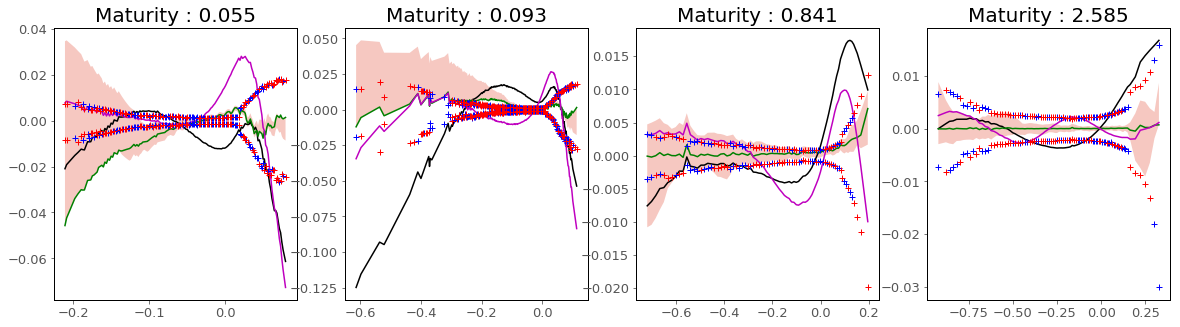
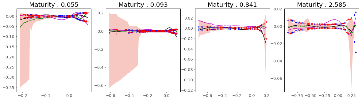
Fig. 3 shows the local volatility surfaces that stem from the three constrained approaches. Fig. 3(a) shows the spiky local volatility surface generated by SSVI, capped at the 200% level for scaling convenience. Fig. 3(b) shows the capped local volatility surface constructed from the GP MAP price estimate. Fig. 3(c) shows the (complete) NN local volatility surface.

The error between the prices of the calibrated models and the market data are evaluated on both the training and the out-of-sample data set. The first two rows of Table 1 compare the in-sample and out-of-sample RMSEs of the prices and implied volatilities across the different approaches. The differences between the training and testing RMSEs are small, suggesting that all approaches are not over-fitting the training set. The GP exhibits the lowest price RMSEs.

The first repricing backtest estimates the prices of the European options corresponding to the testing set, by Monte Carlo sampling in each calibrated local volatility model (same methodology as in [2, Section 7.2]). The second approach uses finite differences to price the options with the calibrated local volatility surfaces. The pricing PDEs with local volatility are discretized using a Crank-Nicolson (CN) scheme implemented on a $100\times 100$ backtesting grid. The last two rows in Table 1 compare the resulting price backtest RMSEs across the different approaches. The NN fitted to implied volatilities exhibit significantly lower errors in the backtests, followed by NN based on prices, SSVI and GP. To quantify discretization error in these backtesting results (as opposed to the part of the error stemming from a wrong local volatility), we ran the same backtests in a Black-Scholes model with 20% volatility and the associated prices. The corresponding Monte Carlo and Crank-Nicholson backtesting IV(price) RMSEs are $2.90\%(1.56)$ and $0.846\%(4.10)$, confirming the significance of the above results.

References

- [1] François Bachoc, Agnes Lagnoux, Andrés F López-Lopera, et al. Maximum likelihood estimation for Gaussian processes under inequality constraints. Electronic Journal of Statistics, 13(2):2921–2969, 2019.
- [2] Marc Chataigner, Stéphane Crépey, and Matthew Dixon. Deep local volatility. Risks, 8(3):82, 2020.
- [3] Areski Cousin, Hassan Maatouk, and Didier Rullière. Kriging of financial term-structures. European J. Oper. Res., 255(2):631–648, 2016.
- [4] Stéphane Crépey and Matthew Dixon. Gaussian process regression for derivative portfolio modeling and application to CVA computations. Journal of Computational Finance, 24(1):47–81, 2020.
- [5] Bruno Dupire. Pricing with a smile. Risk, 7:18–20, 1994.
- [6] Jim Gatheral. The volatility surface: a practitioner’s guide. Wiley, 2011.
- [7] Jim Gatheral and Antoine Jacquier. Arbitrage-free SVI volatility surfaces. Quantitative Finance, 14(1):59–71, 2014.
- [8] Mike Ludkovski and Yuri Saporito. Krighedge: Gaussian process surrogates for delta hedging, 2020. arXiv:2010.08407.
- [9] Hassan Maatouk and Xavier Bay. Gaussian process emulators for computer experiments with inequality constraints. Math. Geosci., 49(5):557–582, 2017.
- [10] K. Murphy. Machine Learning: A Probabilistic Perspective. MIT Press, 2012.
- [11] Johannes Ruf and Weiguan Wang. Neural networks for option pricing and hedging: a literature review. Journal of Computational Finance, 24(1), 2020.
- [12] Martin Tegnér and Stephen Roberts. A probabilistic approach to nonparametric local volatility. arXiv preprint arXiv:1901.06021, 2019.
- [13] Yu Zheng, Yongxin Yang, and Bowei Chen. Gated neural networks for implied volatility surfaces, 2020. arXiv:1904.12834.