X-ray morphology due to charge-exchange emissions used to study the global structure around MarsThanks:
Abstract
Soft x-ray emissions induced by solar wind ions that collide with neutral material in the solar system have been detected around planets, and were proposed as a remote probe for the solar wind interaction with the Martian exosphere. A multi-fluid three-dimensional magneto-hydrodynamic model is adopted to derive the global distributions of solar wind particles. Spherically symmetric exospheric H, H2, He, O, and CO2 density profiles and a sophisticated hybrid model that includes charge-exchange and proton/neutral excitation processes are used to study the low triplet line ratio (0.770.58) of O VII and total x-ray luminosity around Mars. We further calculate the emission factor -value with different neutrals over a wide ion abundance and velocity ranges. Our results are in good agreement with those of previous reports. The evolution of the charge stage of solar wind ions shows that sequential recombination due to charge-exchange can be negligible at the interaction region. This only appears below the altitude of 400 km. The anonymous low disk ratio can be easily explained by the collisional quenching effect at neutral densities higher than 1011cm-3. However, the quenching contribution is small in Mars’ exosphere and only appears below 400 km. Charge-exchange with H2 and N2 is still the most likely reason for this low -ratio. X-ray emissivity maps in collisions with different neutrals differ from each other. A clear bow shock in the collision with all the neutrals is in accordance with previous reports. The resulting total x-ray luminosity of 6.55 MW shows a better agreement with the XMM-Newton observation of 12.81.4 MW than that of previous predictions.
Keywords:
atomic processes – solar wind: individual: Mars-x-raysI Introduction
Solar wind ion–induced charge-exchange (SWCX) x-ray emissions have been detected from most planets in the solar system, e.g., Earth (Snowden et al. 2004)), Mars (Dennerl et al. 2006), Saturn (Branduardi-Raymont et al. 2010), Jupiter (Branduardi-Raymont et al. 2007; Hui et al. 2009). A review of SWCX emission in the solar system was presented by Dennerl et al. 2012. This kind of x-ray emission was further suggested as a probe for remote monitoring of the magnetosheath and magnetopause of the planets and the solar wind by Snowden et al. 2009; Sun et al. 2019 for Earth. Gunell et al. 2004 estimated the SWCX total x-ray luminosity (1.8 MW) to be consistent with the Chandra 2001 observation for Mars that used a hybrid model for the solar wind–Mars interaction and a test particle simulation of heavy ion trajectories near Mars, where a constant cross-section for H and O atoms and a simplified two-step cascade model were adopted. Later, Koutroumpa et al. 2012 performed a three-dimensional (3D) multi-species hybrid simulation model, and reproduced the solar wind–Martian interfaces well by using x-ray morphology, and confirmed its feasibility for the remote probing to the interaction between the solar wind and the Martian exosphere. However, the estimated luminosity of 0.7–2.0 MW is far smaller than the total observed luminosity of 12.81.4 MW (Dennerl et al. 2006). Koutroumpa et al. 2012 included three neutral profiles of H, O, and CO2 in the Martian environment and constant cross-sections with H and H2O without the H2 and He components. Additionally, an anonymous low line intensity ratio of O VII in disk observation cannot be explained by the charge-exchange process.
In this work we incorporate recent progress on solar wind ions distributions from a multi-fluid magneto-hydrodynamic (MHD) simulation comparing with the Mars Atmosphere and Volatile Evolution (MAVEN) spacecraft data. Furthermore, we include more neutral components in the Martian exosphere to re-study the x-ray luminosity. In section 2 we describe the MHD model for solar wind ions, the neutral profile, as well as a sophisticated hybrid atomic model for x-ray emission. In section 3 we present the temperature- and velocity-dependent -value, the evolution of charge-stage of solar wind ions, the collisional quenching effect on line ratios of O VII, and the x-ray emissivity maps in the XZ plane. Finally, a summary and conclusion are outlined in section 4.
II Simulation model
In this interaction of solar wind ions with Martian neutrals (including H, H2, He, O, CO2), the local volume emission rate from charged ion is given by Cravens 1997; Koutroumpa et al. 2009,
| (1) |
where is number density of solar wind ions at given location (, ), respectively. is the line emissivity at a relative collisional velocity between solar wind ion and -th neutral. Here is the bulk velocity of the solar wind and the second term is the general thermal velocity. The number density of different charged ions is a self-consistent solution to the differential equation:
| (2) | |||||
that describes the evolution of solar wind charged ions in the radial direction, where the initial ion number density is defined by its abundance in the solar wind before interaction.
II.1 Neutral atmosphere and exosphere
The Martian neutral environment is composed of CO2, O, H, H2, He, and N2 as shown in Fig. 1. The density profiles of CO2, and O are fit to results from the Mars thermosphere global circulation model (MTGCM) as reported by Koutroumpa et al. 2012. The hydrogen density profile is fit to results from Anderson & Hord 1971 and Krasnopolsky 2002 and can be written by
| (3) | |||||
For the H2 and He density profile we adopt the results of Krasnopolsky 2010with a similar fitting formula as H but with different fitting parameters as given by
| (4) | |||||
| (5) | |||||
The fitting values at low altitudes are consistent with the results of Krasnopolsky 2010.
Recently, these neutral profiles below 500 km have been measured by the Neutral Gas and Ion Mass Spectrometer (NGIMS) on the Mars Atmosphere and Volatile EvolutioN (MAVEN) mission (Mahaffy et al. 2015; Stone et al. 2022; Wu et al. 2021). The hydrogen profile was measured via the 1216 Å Lyman alpha line covered by the Imaging Ultraviolet Spectrograph (IUVS) on the MAVEN mission (Chaffin et al. 2018). Stone et al. 2022 further investigated their horizontal variations with local time, latitude and season. The magnitude of variation is very large, and even more than an order of magnitude for H2 and He (Stone et al. 2022, see Fig. 6 there). For comparison, the MAVEN measurements during the orbit period of DD2 (Wu et al. 2021; Stone et al. 2022) and similar fitting as above are presented in the bottom panel of Fig. 1. Since there are not in-situ measurement data for the neutral density above 1000 km, we still can not calibrate the uncertainty of this extrapolation. Yet it approximately follows the relation of (here is the hydrogen density near Mars). Although their proportional relation to the x-ray emission as shown in Eq.(2), the low neutral density at distant halo region makes the resultant total X-ray luminosity to be affected smalle by the uncertainty of this extrapolation. By using the two different groups of the neutral profiles, we will estimate the uncertainty of the total luminosity from neutrals, that will be discussed in the following discussion section.

II.2 Global distribution of solar wind ions around Mars
The interaction of the solar wind with the Martian atmosphere and ionosphere results in the formation of two distinct boundaries, i.e., bow shock and magnetic pileup (or magnetic pause). Modolo et al. 2005; Modolo et al. 2006 investigated the global structure around Mars using a three-dimensional multi-species (proton and He2+) hybrid model, where complicated substructures were demonstrated in density maps of protons and -particles. Using the MAVEN spacecraft data and an algorithm of automated region identification, N ˇ e mec et al. 2020 derived an empirical model for both the bow shock and magnetic pileup boundary locations around Mars. By assuming cylindrical symmetry, a parabolic model with a focus on the subsolar standoff location () in the -axis (Sun-Mars center line) can well fit the two boundaries, i.e.,
| (6) |
Here, and (in ) are aberration-corrected cylindrical coordinates of a given point at the bow shock and magnetic pileup boundary. , , , , and are parameters fit to the MAVEN spacecraft data for the bow shock and magnetic pileup boundary. is dynamic pressure in nPa, refers to the solar ionizing flux in mW m-2, and denotes the magnitude of the magnetic field in n. The best-fit result for the bow shock and magnetic pileup boundary are illustrated by thick black curves in Fig. 2.
In this work a multi-fluid 3D MHD model is adopted to derive the global distributions of the solar wind particle (H+) density and velocity surrounding Mars, where the Navier-Stoker equations for five significant ion species (i.e., proton in solar wind, H+ from Mars, O, O+, CO) in the Martian ionosphere were used to describe the physics. The equations include conservation equations for the plasma flow with respect to continuity, momentum, and energy. The Navier-Stoker equations for each species are augmented by the interaction of the electromagnetic effects. The physical detail for this 3D MHD model can be found in the studies of Li et al. 2020; Li et al. 2022.
The computational domain is -24 , -16 , where is the radius of Mars ( km). Because the general curvilinear coordinate system is adopted, a high resolution for the region with the most intense variations of physical parameters is achieved by refining the physical grid, and the smallest grid size can approach 60 km. The solar wind density and velocity are chosen to be 4 cm-3 and 500 km/s, respectively. The interplanetary magnetic field (IMF) is chosen to be 3 nT.
The solar wind density and velocity profiles in the XZ-plane show a clear bow shock with its position being excellent agreement with that from MAVEN spacecraft data (N ˇ e mec et al. 2020), see Fig. 2.


II.3 Emission model
To calculate the line emissivity of at a given location (, ) due to charge-exchange electron captures with neutrals, and to calculate subsequent radiative decays, either directly to the ground and lower excited states or via cascades, we obtain the density of an ion at a given -th level state by solving the following rate equation assuming equilibrium:
| (7) | |||
where is the number density of charged ions at -th level state, while corresponds to the number density of kind of neutrals, e.g. H, H2, He, O, and CO2. refers to the density of H. and are the single and double-electron capture rate coefficients, respectively. is the radiative decay rate for a given transition line . are the proton impact excitation rates at a given temperature that are used to account for neutral impact excitations due to high density at lower altitudes, and are only considered for O VII triplets at disk observation. is the relative collision velocity between and kind of neutrals, while and are the cross-section of single- and double-electron transfer processes. refers to the ratio of ionic fraction between and charged ions before electron capture. Furthermore, the line emissivity can be obtained.
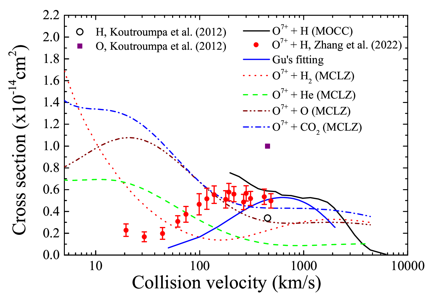
The atomic data of level energies and radiative decays have been reported by Liang et al. 2014; Liang et al. 2021. Here the charge-exchange cross-sections are from the Kronos v3.1 database 11 1 www.physast.uga.edu/research/stancil-group/atomic-molecular-databases/kronos that is implemented by Stancil research group in a series of studies (Cumbee et al. 2014; Cumbee et al. 2018; Mullen et al. 2016; Mullen et al. 2017) that use multiple methods, including multichannel Landau-Zener (MCLZ), atomic-orbital close-coupling (AOCC), molecular-orbital close-coupling (MOCC), and classical trajectory Monte Carlo methods. For the collision of O7+ with the O atom, there are no data available. Hence, the MCLZ CX cross-section of O7+ with water (H2O) is used because of their similar weight. For the double-electron capture cross-section, we adopt those available data that are explained in the study by Liang et al. 2021. Since the data availability from AOCC/MOCC method are in the Kronos database, we adopt cross-sections from the AOCC/MOCC method for bare- and H-like ion collisions with the hydrogen or helium atom, while data from the MCLZ method will be used for collisions with other neutrals. This means the velocity-dependent CX cross-section is used in this work, not the constant cross-section used in the work of Koutroumpa et al. 2012. For example, Fig. 3 shows the cross-section of H-like oxygen O7+ ion collisions with different neutrals in the Martian exosphere. For comparison the values used by Koutroumpa et al. 2012 are also plotted; these values have a smaller cross-section with H and a larger cross-section with O than the accurate calculation in Kronos v3 database by 40% and 300% respectively, and were used by Koutroumpa et al. 2012. Therefore, the x-ray emissions would be under-/over-estimated in this previous work. In the collision with H, Zhang et al. 2022 measured the absolute cross-sections at collisional velocities covering the typical solar wind velocities; see symbols with error bars in Fig. 3. Thus, these experimental data in the collision with H are used in this work. There is an obvious difference between the experimental results and the theoretical calculations including those from Kronos database and from Gu’s fitting below 200 km/s. This illustrates that a sophisticated method and laboratory measurements are still required for the velocity-dependent cross-sections in the collisions with other neutrals, even the best available cross-sections are used in this paper. This kind of uncertainty has a significant effect on spectral analyses for observations with high-resolution by using the charge-exchange model, and has been pointed out by Gu et al. 2022 for advanced theoretical calculations for especially the low collision energy regime, in combination with more laboratory measurements.
III Results and Discussion
III.1 Velocity and temperature dependence of value
The -value combined with MHD modeling is extensively used by the space physics community. This is a proportional factor based on a combination of the relative abundances and the cross-section of each possible interaction between a solar wind ion and a neutral particle causing line emissions as defined by Cravens 1997 and Whittaker et al. 2016 as follows:
| (8) |
where ion emissivity of a charged ion is obtained by summing the line emissivity with the neutral particle of for a given transition . The line emissivity of one solar wind species can be obtained from Eq. (7) at the collision with the neutral by multiplying by the radiative rate . In previous works (Schwadron & Cravens 2000; Cravens 1997; Whittaker & Sembay 2016), the line emissivity in Eq. (8) is replaced by , which means cascading effects to the upper atomic states of the transition have been neglected.
Eq. (8) shows that the -value is highly variable depending on the ionic fraction of a given element and its abundance. Due to the extreme low electron density in inter-planetary space, the charge state distribution of solar wind ions will freeze-in after leaving the solar surface (Landi et al. 2012). This distribution in the solar wind provides insight into its origin with the characteristic temperature from the Sun. Thus, we adopt the temperature in collisional equilibrium to represent the relative ionic fraction in solar wind. Figure 4 shows the -values (in eV cm2) of oxygen in collisions with different neutrals (e.g., H, H2, He, O and CO2) as a function of solar wind velocity and logarithmic temperature (in the unit of K). Here, the solar abundance of Lodders et al. 2009 is adopted with oxygen to hydrogen abundance ratio of [O/H]=6.05, which is slightly higher than the mean values ranging from 2.03 to 4.76 from the ACE SWICS data for fast and slow solar winds (Whittaker & Sembay 2016), but consistent with the reported mean [O/H] ratio of 3.94 with a standard deviation of 3.01 by Whittaker et al. 2016 from the OMNI data 22 2 https://omniweb.gsfc.nasa.gov/. By using the ACE (Advanced Composition Expoloer) data (including the ion density of O7+,8+, oxygen abundance [O/H], and solar wind velocity) obtained over 13 years (1998–2011) and the charge-exchange cross-sections from Bodewits 2007, the resulting -value has a modal peak at eV cm2 when colliding with hydrogen (Whittaker & Sembay 2016, see Fig. 2). To compare with empirical methods Whittaker et al. 2016 derived an -value of 7.6 eV cm2 by using [O/H]=1.1, an O7+ abundance of 0.28, and an O8+ abundance of 0.05. The present calculation (7.3 eV cm2) shows an excellent agreement with the value measured at the temperature corresponding to the O7+,8+ abundance ratio at equilibrium. The present calculation of log()/K=6.1 shows a good agreement with that of Whittaker & Sembay 2016 at a typical solar wind velocity of 300–600 km/s, where in-situ ACE data including velocity, O7+,8+ abundance, and abundance ratio [O/H], were used. Both the present calculations and previous work from ACE data demonstrate that there is a strong dependence on the ionic fraction or temperature between log()/K=6.0 and 6.5.


Hydrogen gas (H2), He, O, and CO2 are also important components in the Martian neutral environment. Both the multi-fluid 3D MHD computation performed by Li et al. 2020 and MAVEN data demonstrate that the bow shock and magnetic pileup boundary are approximately 1.55 (corresponding to the altitude of 1868 km 33 3 In the unit of the Martian radius , this value is relative to Mars’ center, otherwise it refers to the altitude relative to the Martian surface.) and 1.3 (1018 km) in the direction of Sun to Mars, respectively, see Fig. 2. Below this altitude the number densities of H2 and He become dominant and are higher than those of atomic hydrogen, see Fig. 1. We also present the -value in collision with other Martian neutrals. An obvious dependence on solar wind velocity appears below 200-300 km/s. Large decrease of solar wind velocity after bow shock as shown in Fig 2 reveals that the constant -value adopted in previous works should generate large uncertainties (Whittaker & Sembay 2016; Whittaker et al. 2016). The present calculation will help improve the estimation of x-ray emission in the interaction region. In the calculated temperature and velocity grids the -value with H2, O, and CO2 is systematically higher than the value in the collision with H.
We further calculate the -value of carbon, nitrogen and neon in the collisions with H, H2, He, O, and CO2, see Fig. 5. Compared to the -value of oxygen, the carbon -value is lower than that of oxygen, while the nitrogen -value is even lower. This is mainly resultant from the higher abundance of oxygen than carbon and nitrogen in the solar wind. According to the mean abundance from ACE data of highly charged oxygen ions (O8+/0.28, O7+/0.05, Whittaker et al. 2016) and carbon ions (C6+/0.13, C5+/0.37, Koutroumpa et al. 2012), the calculated -values in the collisions with H are about 7.9 eV cm2 (O) and 4.4 eV cm2 (C), respectively. With the similar temperature of log, the nitrogen -value is eV cm2. We also notice that there is a sudden decrease around 900 km/s for the -value of N in the collision with H. This is due to the recommended -selective cross-section used (Wu et al. 2011, see Fig. 5 there), and its complicated -distribution along the collisional velocity.


III.2 Evolution of charge stage of solar wind ion
To examine the validity of the -value that comes from a specified ion abundance at the interaction region, we calculate the evolution of charge stage of solar wind ions of carbon, nitrogen, and oxygen as defined by Eq. (2). Here, the initial ion abundances are from published literature, for example, Schwadron & Cravens 2000 for oxygen, and Koutroumpa et al. 2012 for carbon. Because the evolution profile of nitrogen ions are similar to those of carbon and oxygen ions, only bare and H-like carbon and oxygen ions in the solar wind are given. For this we considered the resulting soft x-ray emissions within a photon energy range of 200–1000 eV, see Fig. 6. This figure shows that the charge stage distribution of solar wind ions does not change over the interaction region between the bow shock (1.57) and magnetic pileup boundary (1.3). This indicates that there is no sequential recombination due to charge-exchange when the solar wind ion passes through this interaction region. At an altitude of 400 km the relative ion abundance of solar wind carbon and oxygen ions starts to change, and reaches a peak ion abundance for H-like ions at the altitude of 230 km; in other words solar wind ions move slowly, captured H-like ions accumulate and then further sequential recombination take places below 400 km. By using MAVEN DD2 data for the neutral density (Wu et al. 2021), such rising does not appears, that is ion accumulation and sequential recombination do not take place. This is probably due to the lower oxygen density below 300 km in the MAVEN DD2 data. The evolution behavior of highly charged solar wind ions also indicates that the general fixed -value for a given ion abundance is still valid in the interaction region, but it fails below 400 km of Mars.

III.3 Collisional quenching effect on He-like triplet ratio of O VII
The triplet-to-single line intensity ratio (, here is inter-combination, forbidden, and resonance line, respectively) of He-like ions is an important probe for the charge-exchange and/or coronal emissions of astrophysical plasmas, and is used extensively by those who appy astrophysical x-ray spectroscopy with high-resolution (Katsuda et al. 2012; Zhang et al. 2014) to study the interface of hot outflows and cold interstellar (or intergalactic) medium. From the high-resolution XMM-Newton observations of Mars, Dennerl et al. 2006 and Koutroumpa et al. 2012 extracted out these line fluxes for disk and halo regions with ratios of 0.770.58 (disk) and 5.365.82, respectively. The mean value of the ratio for the halo is significantly higher than value for the disk. Many charge-exchange emission models have been setup to explain the large ratio. Mullen et al. 2017 and Cumbee et al. 2018 listed such velocity-dependent ratios of O VII for collisions with different neutrals. For comparison, we also plot these ratios in the left panel of Fig. 7. The present calculation for collisions with H shows a favorable agreement with the halo mean value and theory from Bodewits et al. 2007. Due to the low signal-to-noise ratio, the halo ratio has large error bars (Fig. 7). This will be clarified by next-generation X-ray missions, e.g., XRISM 44 4 https://heasarc.gsfc.nasa.gov/docs/xrism/about/, Athena 55 5 https://www.cosmos.esa.int/web/athena and HUBS 66 6 http://hubs.phys.tsinghua.edu.cn/en/index.html.


For the disk ratio of 0.770.58 the charge-exchange model from Mullen et al. 2017 when colliding with nitrogen and hydrogen gases (N2 and H2) gives ratios ranging from 1.0 to 1.7, which is consistent with disk observations within error bars. Koutroumpa et al. 2012 suggested this low ratio is due to the quenching collisions with neutrals, that will remove excited electrons from the long-lived metastable states, then suppress the line intensity. Their qualitative analysis for the collisional effect is clear below 150 km, and they estimated the contribution from below 150 km to be less than 15%. In this work we performed a detailed calculation by including excitations from heavy particles in Eq. (7). However, neutral impact excitation data of highly charged ions are very scarce, even the proton impact excitation of highly charged ions is available for just a few cases. Seaton 1955; Seaton 1964 presented the theory of proton impact excitation, and applied it to the green coronal line of Fe13+for the transition. When the excitation energy is much smaller than the plasma temperature , the proton excitation rate would be greater than the electron impact by a factor of order , being the proton mass and the electron mass (Dalgarno 1983). The excitation energy of O VII from metastable level (1s2s ) to 1s2p levels is 10–16 eV, which is far smaller than the plasma temperature of 110 eV. Thus, we derived the proton (neutral) impact excitation (PIE) rates from the metastable level of O VII by using the electron impact excitation rates in the sasal database (Liang et al. 2014; Takabe et al. 2008).
According to Eq. (7) we calculate the ratio of O VII with a pure charge-exchange model and a hybrid one (e.g. CX plus proton impact excitation) in the collisions with H, H2, and He, respectively. From the right panel of Fig. 7, we see that the ratio from the hybrid model starts to deviate from the pure CX one when above the neutral density of 106 cm-3, and becomes more obvious as the neutral density increases. According to the neutral profile presented in Fig. 1, the collisional quenching effect appears below the altitude of 400 km through the collisional excitations by neutral oxygen and/or CO2. Figure 7 also indicates that the ratios from the pure CX calculation with different neutrals disperse strongly, for example, 5.3 (H), 2.7 (He), and 0.98 (H2). However, the disk observation of Mars reported by Dennerl et al. 2006) covers the photons within 10, that is below altitude of 2180 km. Above 400 km and below 2000 km altitude H2, He, and O are dominant components in the Martian atmosphere with density of —2 cm-3. From Fig. 9 and Fig. 10 discussed in next subsection, we can see that the disk observation (white dotted circle) covers more than 86% of the emission energies, where the emissivities from H2 and O are comparable to or higher than those from H at lower altitudes. Both their contributions can be up to 43% and 65%, respectively. Thus, we suggest the pure CX with H2 and O may be the part of the reason for the low disk observation of 0.770.58.
By including all the neutral components in Eq.(7) we can further calculate the map of triplet line ratios with a pure charge-exchange and a hybrid one as illustrated in Fig. 8. Here, only the hybrid calculation is presented due to both maps have basically the same distribution except for data below 200 km which show small differences. Hence, the proton impact excitation may not be the main reason for the low disk observation of 0.770.58. In this figure, the nearly spherical symmetry of the ratio follows the neutral profiles used in this work. It is obvious that the G ratio decreases with decreasing altitude, and it reaches a low value of 2.8 at altitude of 700 km. Within the main region of disk observation reported by Dennerl et al. 2006, the ratio is approximately 2.8–3.4, which is still higher than the disk observation. By using the in-situ MAVEN measurements for neutrals shown in the bottom panel of Fig. 1, the ratio changes slightly to 2.2–3.0. This decreasing trend of the -ratio indicates that the contributions from H2 and O steadily increase and become significant, but still not absolutely dominant. This is consistent with the x-ray luminosity profiles shown in Fig. 10, which will be discussed in the next subsection. When the solar wind bulk velocity is used, the -ratio can reach a low value of 0.9 at the altitude of 400 km. The higher cross-section below 100 km/s in the collision with H2 (see Fig. 3) and the low bulk velocity (100 km/s, see Fig. 2), is the reason for the low calculated -ratio of 0.9. Therefore, we suggest that the charge-exchange with H2 gas may still be the possible reason for the low disk observation. Such dependence of the ratio on the altitude can be explored by future deep observations with next generation x-ray missions with high efficiency (e.g. XRISM 4, Athena 5 and HUBS 6). We also notice that there is a tail-like feature for the -ratio by using the bulk velocity of the solar wind, that is consistent with the tail-like feature in the bulk velocity map shown in Fig. 2. Then we think this tail-like feature in the -ratio is resultant from the low bulk velocities and relative higher cross-sections at low collisional velocities with the multiple-electron neutrals (e.g. H2, He and O) as shown in Fig. 3. By considering the observed ratio derived from the observed flux in the line of sight, the ratio map is weighted by projected flux in different direction of line of sight (LOS) discussed in Sect. 3.5, then we obtain the expected ratio of 1.6–1.8 in the disk observation, see Table 1. That is slightly higher than the disk observation of 0.770.58. It should be noted that the present charge exchange cross sections are the best ones available, but not the best ones qualified to use for high-resolution spectroscopy; these need more elaborate benchmark measurements for the selective cross section for its extensive application in the near future.


III.4 Contribution of different neutrals on x-ray emissivity distribution in the XZ plane
In view of the different neutral profiles as shown in Fig. 1 and different charge-exchange cross-sections as shown in Fig. 3, we begin by investigating the contribution from different neutrals to the x-ray emissivity distribution in the XZ-plane (Fig. 9). The spatial distribution of x-ray emissivities shows obvious differences in collisions with different neutrals. On the whole the x-ray emissivity distribution for the collisions with H shows an obvious bow shock in the XZ-plane, consistent with that derived from MAVEN spacecraft data (N ˇ e mec et al. 2020, solid white curves) and the density map from the MHD simulation. Weak x-ray emissions extend toward the solar direction in the longer region and toward the far region in magnetosheath. However, the bright x-ray emissions in the collisions with H2 (with peak value of 1.5 erg cm-3s-1) concentrate in the region near the magnetic pileup boundary with less extension toward the magnetosheath, and are higher than those from the H collision between 1.15–1.32 (Fig. 10). The contributions of the He collision are mainly below 1.17 with emissivity values much smaller than those of the H and H2 collision. Since the oxygen and carbon-dioxide become the dominant components of the Martian atmosphere below the altitude of (550 km), the main x-ray contribution is from the collision with O with emissivity values comparable to those of H collisions, as shown by the dark-blue curve in Fig. 10. For a clear inspection we further present the profile of x-ray emissivities at four different directions (0∘, 30∘, 60∘ and 90∘) relative to the Sun-to-Mars line (Fig. 10). Basically, the contributors to x-ray emissivity profiles follow the neutral profiles in the Martian environment with some difference in detail.


By considering the consistency of x-ray emissivity distribution with the structure of solar wind interaction with the Martian exosphere, the present work confirms again that x-rays can be used to probe the global structure of solar wind interaction with planets (Snowden et al. 2004; Snowden et al. 2009; Sun et al. 2019). The different contribution profiles and line features in x-rays with different neutrals suggest that x-ray spectroscopy can probe the neutral components with future deep observations with spatial and energy resolutions that can be achieved by next generation x-ray missions, such as XRISM 4, Athena 5 and HUBS 6.
III.5 X-ray morphology of Mars
The same procedure is used for carbon and nitrogen emissions with ion fractions of 0.13 (C6+)77 7 From real-time measurement of ACE-SWICS, see Table 1 in the work of Koutroumpa et al. 2012 , 0.37 (C5+)7, 0.006 (N7+), and 0.058 (N6+). We calculate the x-ray emissivities in the energy range between 200—1000 eV for the three-dimensional distribution of carbon, nitrogen, and oxygen ions within 8.3 (55) of Mars. Since there are not emission lines from captured H- and He-like carbon, nitrogen and oxygen ions in the ranges of 200–300 eV and 900–1000 eV (Koutroumpa et al. 2006; Liang et al. 2021, see Table 1 and Fig. 10 there, respectively), the present energy range is consistent with that (300–900 eV) in the XMM-Newton observation and previous works (Koutroumpa et al. 2012). We obtain the x-ray morphology and total x-ray luminosity around Mars (Fig. 12) by integrating along the -direction (Martian motion) and summing in this projected plane as following:
| (9) | |||
| (10) |
where refers to the projected emission flux (in the unit of erg cm-2 s-1) in -direction with integration range between -8.3 and 8.3, yet those emissions from the region with are blocked by Mars in this projection plot. The summations are for above listed elements, as well as H- and He-like captured ions that emits x-ray photons. is the total SWCX luminosity by integrating the emissivity within a cubic box with the size of 16.6 (or ). The emission rate or of one charged ion is defined by Eq.(1) in the previous model section.
The resulting total SWCX x-ray luminosity is 6.55 MW (O: 3.01, C: 2.69 and N: 0.85 MW, respectively) in this work, showing a better agreement with the XMM-Newton observation of 12.81.4 than previous predictions. Koutroumpa et al. 2012 made some estimations for the additional x-ray luminosity, e.g., larger simulation box (8 ) with an additional 5%, average abundance of solar wind which is three times higher than their usual value, with He and H2 contributions in the disk region. After these additional contributions their simulated x-ray luminosity can reach between 1.2 and 2.0 MW. They also pointed out a halo coronal mass ejection (CME) event on 2003/11/18 as perhaps a possible explanation. A strong ion flux on average 18 times real-time values in their simulation could yield a total luminosity of 6.3 MW, that is in better agreement with, but still quite lower than, the observed value of 12.81.4 MW.
In this observed luminosity, assumptions of isotropic emission and optically thin were used by multiplying the observed fluxes of emission lines with (here AU is the distance between Earth and Mars) (Dennerl et al. 2006; Koutroumpa et al. 2012). Contribution from fluorescent scattering of solar x-rays has not be included (Dennerl et al. 2006). By using the observed fluxes of the fluorescence lines from and transitions of CO2 around 525 eV, the fluorescent luminosity was derived to be 3.41.4 MW by Dennerl et al. 2006, being approximately 27% of the total SWCX luminosity of 12.81.4 MW.
We further calculate total SWCX luminosity contributions at different layers (with a step of 0.5 ) by using the oxygen emissivity with all listed neutrals, see Fig. 13. The contribution from the interaction region () is the largest emission source () with the minimum emitting volume. While the emissivities shown in Fig. 9 become smaller with increasing altitude, the emitting volume increases as , resulting in the luminosity contributions to increase again after . The luminosity contribution between 43 () and 50 radius () is , being higher than the crude estimation (5%) of Koutroumpa et al. 2012. This illustrates that the uncertainty of neutrals at high altitude has a non-negligible effect on the total luminosity. However, the absence of in-situ measurement for the hydrogen density at higher altitudes limits the examination for the present calculation.
By using a different group of neutral densities, e.g. in-situ MAVEN measurement at the orbit period of DD2 (Stone et al. 2022; Wu et al. 2021), we re-calculate the total CXE luminosity to be 5.93 MW being smaller than the former calculation by 10%. Although there are large differences for the neutral densities at low altitude shown in Fig. 1, the resultant total SWCX luminosity does not change a lot. Figure 1 illustrates that SWCX emission is dominantly from the collision with hydrogen at , where the hydrogen density is very close between the fitting to MAVEN DD2 data and the fitting given by Eq. (3). The small difference of the calculated luminosities indirectly indicates that the emission from distant halo regions with large volume around Mars plays an non-negligible role on the observed luminosity, that is consistent with the discussion for the radial distribution of the luminosity, as shown in Fig. 13.
By using the in-situ solar wind data from ACE Science Center Level 2 database 88 8 https://www.swpc.noaa.gov/products/ace-real-time-solar-wind, we estimate the time delay () of the solar wind to be about 45–53 hours between the L1 point (ACE position) and Mars by using with of 600–710 km/s and =0.77 AU (Koutroumpa et al. 2012). This corresponds approximately to the window between 2003/11/18 05:00 UT and 2003/11/19 10:00 UT for the solar wind event around Mars, during the XMM-Newton observation (Dennerl et al. 2006), see Fig. 11. The solar wind velocity decreases from 710 to 530 km/s, yet the density holds basically a constant value of 2.7 cm-3 till 2003/11/19 00:00 UT, then increases to 5.0 cm-3 at the end of above window. By considering the difference between the in-situ ACE measurements and the values used in this work, the total SWCX luminosity varies in the range of 6.28–8.68 MW. When the solar wind density is further scaled to Mars’ heliocentric distance (1.43 AU) by , the total luminosity decreases to 3.1–4.3 MW. During this period, the solar wind state changes slightly at Mars, see gray shadow region in the third panel of Fig. 11. By using the ACE measured oxygen abundance and the charge state (Bonamentel et al. 2021), we further calculate the -value of oxygen, that shows a mean value of (1.4–6.6) eV cm2 from the beginning till the end of the event window at Mars, that is slightly lower than the value of 7.3 eV cm2 adopted in our work, see the discussion at Sect.3.1. That is the resultant total luminosity should be decreased again slightly.

Another possible reason is the assumption of isotropic emission used to derive the observed luminosity by Dennerl et al. 2006. The projected x-ray flux shown in the left panel of Fig. 12 illustrates that there is an obvious non-isotropic feature for the dayside and nightside. By considering the observed flux from a specified phase angle () adopted to derive the luminosity, we calculate the mean value for the projected x-ray emission flux within the disk region (15 radius) at different phase angles, see Table 1. It shows that the mean projected flux varies within 4.5–5.7 erg cm-2 s-1. Then we suggested the observed luminosity of 12.81.4 might be overestimated by 20%.
| Phase | ratio | Projected flux |
|---|---|---|
| angle | erg cm-2 s-1 | |
| 90∘ | 1.75 | 5.60 |
| 60∘ | 1.63 | 4.52 |
| 40∘ | 1.75 | 5.61 |
| 0∘ | 1.68 | 4.79 |
| 120∘ | 1.64 | 4.49 |
| 140∘ | 1.74 | 5.66 |
| 180∘ | 1.68 | 4.76 |
In summary, the total SWCX luminosity is closely related to the solar wind condition and the planetary environment, that can be used to study the neutral density when the real-time information is available for the solar wind.


IV Summary and conclusion
In this study, using the newest charge-exchange cross section in Kronos v3.1 and experimental measurements, we calculate the emission factor -value of carbon, nitrogen, and oxygen with different neutrals (H, He, H2, O, and CO2) in the Martian environment over wide temperature and velocity ranges. The -value is highly variable over a temperature range of log()/K=5.9—6.4 for oxygen, which shows an obvious dependence on velocity below 200–300 km/s. Both the MHD simulation and in-situ MAVEN measurements reveal that the bulk velocity of solar wind decreases to below 100 km/s after the bow shock. Then the general single -value is not valid again. Overall, the -value in collisions with O and CO2 is higher than with others, e.g., H and He. The present -value of oxygen agrees well with previous reports in the collisions with H at the temperature of log()/K=6.1 and typical solar wind velocity of 300–600 km/s. The evolution of charge stage of solar wind ions shows that there is not a sequential recombination from charge-exchange across the interaction region; H-like ion pileups and sequential recombination appear below the altitude of 400 km. This indicates again that the general fixed -value is not valid below this altitude.
By considering the excitation energy (10–16 eV) from the metastable level to higher levels, we obtain the proton impact excitation cross sections from electron impact excitation data based on the theory of Seaton 1955. Then we incorporate them into a sophisticated hybrid emission model. Furthermore, the anonymous low disk ratio (0.770.58) was explored, and can be directly explained by the collisional quenching effect due to proton/neutral collisions. However, the quenching contribution is small for the disk observation and only appears below 400 km. Hence, we suggest that charge-exchange with H2 and N2 may be the most likely reason for this low mean -ratio with large error-bars.
We also presented x-ray emissivity maps from solar wind ions impinging on different neutrals in the Martian exosphere, which is in accordance with bow shock derived from in-situ MAVEN solar wind ion density and velocity mapping. The contributions from different collisional neutrals are explored, which are shown to differ from each other. The resulting total x-ray luminosity of 6.55 MW shows a better agreement with the XMM-Newton observation of 12.81.4 MW than previous ones. Its dependences on solar wind variation and neutral density profile around Mars are discussed.
We present a detailed study for x-rays due to charge-exchange around Mars. This reconfirms that x-rays represent a good remote sensor for the global interaction of solar wind with a planetary atmosphere. This study illustrates an example of charge-exchange emissions in space physics, and shows a requirement for benchmarks for data of selective velocity-dependent charge-exchange cross-section.
References
- Anderson & Hord (1971) Anderson, D.E., & Hord, C.W. 1971, J. Geophys. Res., 76, 6666
- Bodewits (2007) Bodewits, D. 2007, PhD thesis, Univ. of Groingen, Netherlands.
- Bodewits et al. (2007) Bodewits, D., Christian, D.J., Torney, M., Dryer, M., Lisse, C.M., Dennerl, K., et al. 2007, A&A, 469, 1183–1195
- Bonamentel et al. (2021) Bonamente, E., Christian, D.J., Xing, Z., Venkataramani, K., Koutroumpa, D., Bodewits, D. 2021, Planetary Science Journal, 2, 224
- Bougher et al. (2015) Bougher, S.W., Pawlowski, D., Bell, J.M., Nelli, S., McDunn, T., et al. 2015, J. Geophysical Research: Planets, 120, 311–342
- Branduardi-Raymont et al. (2007) Branduardi-Raymont, G., Bhardwaj, A., Elsner, R.F., Gladstone, G.R., et al. 2007, A&A, 463, 761–774
- Branduardi-Raymont et al. (2010) Branduardi-Raymont, G., Bhardwaj, A., Elsner, R.F., and Rodriguez, P. 2010, A&A, 510, A73
- Chaffin et al. (2018) Chaffin, M.S., Chaufray, J.Y., Delghan, J., Schnelder, N.M., Mayyasi, M., et al. 2018, J. Geophys. Res: Planets, 123, 2192–2210
- Cravens (1997) Cravens, E.T. 1997, Geophys. Res. Lett., 24, 105–108
- Cumbee et al. (2014) Cumbee, R.S., Henley, D.B., Stancil, P.C., Shelton, R.L., Nolte, J.L., Wu, Y., Schultz, D.R. 2014, ApJ, 787, L31
- Cumbee et al. (2018) Cumbee, R.S., Mullen, P.D., Lyons, D., Shelton, R.L., Fogle, M., Schultz, D.R., Stancil, P.C. 2018 ApJ, 852, 7
- Dalgarno (1983) Dalgarno, A., 1983, Atoms in Astrophysics, Edited by Burke, P.G., Eissner, W.B., Hummer, D.G., Percival, I.C., Plenum Press, New York and London, p103–112
- Dennerl et al. (2002) Dennerl, K. 2002, A&A, 394, 1119
- Dennerl et al. (2006) Dennerl, K., Lisse, C.M., Bhardwaj, A., Burwitz, V., Englhauser, J., et al. 2006, A&A, 451, 709
- Dennerl et al. (2012) Dennerl, K., Lisse, C.M., Bhardwaj, A., Christian, D.J., Wolk, S.J., Bodewits, D., Zurbuchen, T.H., Combi, M., Lepri, S. 2012, Astron. Nachr., 333, 324–334
- Dizire et al. (2015) Dizire, A., Pelka, A., Ravasio, A., Loupias, B., Falize, E., Kuramitsu, Y., et al. 2015, Phys. Plasmas, 22, 012792
- Gu et al. (2016) Gu, L.Y., Kaastra, J., & Raassen, A.J.J. 2016, A&A, 588, A52
- Gu et al. (2022) Gu, L.Y., Shah, C., & Zhang, R.T. 2022, Sensors, 22, 752
- Gunell et al. (2004) Gunell, H., Holmstrm, M., Kallio, E., Janhunen, P., & Dennerl, K. 2004, Geophysical Research Lett., 31, 22801
- Hui et al. (2009) Hui, Y., Schultz, D.R. Kharchenko, V.A., Stancil, P.C., Cravens, T.E., Lisse, C.M., Dalgarno, A. 2009, ApJ, 702, L158–L162
- Katsuda et al. (2012) Katsuda, S., Tsunemi, H., Mori, K., Uchida, H., Petre, R., Yamada, S., Akamatsu, H., Konami, S., & Tamagawa, T. 2012, ApJ, 756, 49
- Koutroumpa et al. (2006) Koutroumpa, D., Lallement, R., Kharchenko, V., Dalgarno, A., Pepino, R., Izmodenov, V., and Qumerais, E. 2006, A&A, 460, 289–300
- Koutroumpa et al. (2012) Koutroumpa, D., Modolo, R., Chanteur, G., Chaufray, J.-Y., Kharchenko, V., & Lallement, R. 2012, A&A, 545, A153
- Koutroumpa et al. (2009) Koutroumpa, D., Lallement, R., Kharchenko, V., & Dalgarno, A. 2009, Space Sci. Rev., 143, 217–230
- Krasnopolsky (2002) Krasnopolsky, V.A. 2002, Journal of Geophysical Research, 107, 11
- Krasnopolsky (2010) Krasnopolsky, V.A. 2010, Icarus, 207, 638–647
- Li et al. (2020) Li, S.B., Lu, H.Y., Cui, J., Yu, Y.Q., Mazelle, C., Li, Y., Cao, J.B. 2020, Earth and Planetary Physics, 4, 1–9
- Li et al. (2022) Li, S.B., Lu, H.Y., Cao, J.B., Mazelle, C., Cui, J., Rong, Z.J., et al. 2022, ApJ, 931, 30
- Landi et al. (2012) Landi, E., Gresbeck, J.R., Lepri, S.T., Zurbuchen, T.H., & Fisk, L.A. 2012, ApJ, 761, 48
- Liang et al. (2014) Liang, G.Y., Li, F., Wang, F.L., Wu, Y., Zhong, J.Y., Zhao, G. 2014, ApJ, 783, 124
- Liang et al. (2021) Liang, G.Y., Zhu, X.L., Wei, H.G., Yuan, D.W., Zhong, J.Y., Wu, Y., Hutton, R., Cui, W., Ma, X.W., Zhao, G. 2021, MNRAS, 508, 2194–2203
- Lodders et al. (2009) Lodders, K., Palme, H., & Gail, H.-P. 2009, Solar System, Trmper (ed.), Doi: 10.1007/978-3-540-88055-34
- Mahaffy et al. (2015) Mahaffy, P.R., Benna, M., Elrod, M., Yelle, R.V., Bougher, S.W., et al. 2015, Geophys. Res. Lett., 42, 8951–8957
- Modolo et al. (2005) Modolo, R., Chanteur, G.M., Dubinin, E., & Matthews, A.P. 2005, Annales Geophysicae, 23, 433–444
- Modolo et al. (2006) Modolo, R., Chanteur, G.M., Dubinin, E., & Matthews, A.P. 2006, Annales Geophysicae, 24, 3403–3410
- Mullen et al. (2016) Mullen, P.D., Cumbee, R.S., Lyons, D., Stancil, P.C. 2016, ApJS, 224, 31
- Mullen et al. (2017) Mullen, P.D., Cumbee, R.S., Lyons, D., Gu, L., Kaastra, J., Shelton, R.L., & Stancil, P.C. 2017, ApJ, 844, 7
- Nmec et al. (2020) Nmec, F., Linzmayer, V., Nmeek, Z., afrnkov, J. 2020, J. Geophys. Research: Space Physics, 125, e2020JA028509
- Schwadron & Cravens (2000) Schwadron, N.A., & Cravens, T.E. 2000, ApJ, 544, 558–566
- Seaton (1955) Seaton, M.J. 1955, Proc. Phys. Soc. A, 68, 457
- Seaton (1964) Seaton, M.J. 1964, MNRAS, 127, 191
- Snowden et al. (2004) Snowden, S.L., Collier, M.R., and Kuntz, K.D. 2004, ApJ, 610, 1182–1190
- Snowden et al. (2009) Snowden, S.L., Collier, M.R., Cravens, T., Kuntz, K.D., Lepri, S.T., Robertson, I., Tomas, L. 2009, ApJ, 691, 372–381
- Stone et al. (2022) Stone, S.W., Yelle, R.V., Benna, M., Elrod, M.K., & Mahaffy, P.R. 2022, J. Geophys. Research: Planets, 127, e2021JE007085
- Sun et al. (2019) Sun, T.R., Wang, C., Sembay, S.F., Lopez, R.E., Escoubet, C.P., et al. 2019, J. Geophys. Res.: Space Phys., 124, 2435–2450
- Takabe et al. (2008) Takabe, H., Kato, T.N., Sakawa, Y., Kuramitsu, Y., Morita, T., et al. 2008, Plasma Phys. Control. Fusion, 50, 124057
- Whittaker & Sembay (2016) Whittaker, I.C., & Sembay, S. 2016, J. Geophys. Res. Lett., 43, 7328–7337
- Whittaker et al. (2016) Whittaker, I.C., Sembay, S., Carter, J.A., Read, A.M., Milan, S.E., & Palmroth, M. 2016, J. Geophys. Research: Space Physics, 121, 4158–4179
- Wu et al. (2021) Wu, X.S., Cui, J., Niu, D.D., Ren, Z.P., & Wei, Y. 2021, ApJ, 923, 29
- Wu et al. (2011) Wu, Y., Stancil, P.C., Liebermann, H.P., Funke, P., Rai, S.N., et al. 2011, Phys. Rev. A, 84, 022711
- Zhang et al. (2014) Zhang, S.N., Wang, Q.D., Ji, L., Smith, R.K., Foster, A., & Zhou, X. 2014, ApJ, 794, 61
- Zhang et al. (2022) Zhang, R.T., Seely, D.G., Andrianarijaona, V.M., Dragani, I.N., et al. 2022, ApJ, 931, 1