Inflation in Metric-Affine Quadratic Gravity
Abstract
In the general framework of Metric-Affine theories of gravity, where the metric and the connection are independent variables, we consider actions quadratic in the Ricci scalar curvature and the Holst invariant (the contraction of the Riemann curvature with the Levi-Civita antisymmetric tensor) coupled non-minimally to a scalar field. We study the profile of the equivalent effective metric theory, featuring an extra dynamical pseudoscalar degree of freedom, and show that it reduces to an effective single-field inflationary model. We analyze in detail the inflationary predictions and find that they fall within the latest observational bounds for a wide range of parameters, allowing for an increase in the tensor-to-scalar ratio. The spectral index can either decrease or increase depending on the position in parameter space.
1 Introduction
Cosmological inflation [1, 2, 3, 4, 5, 6, 7], according to which the Universe underwent a phase of quasi-de Sitter expansion, has become central to our present understanding of early Cosmology primarily because it provides a mechanism for the origin of formation of the observed large scale structure [8, 9, 10, 11, 12, 13]. A standard way to model inflation is to introduce a scalar field (the inflaton) that on the one hand provides the vacuum energy driving the expansion and on the other hand through its quantum treatment generates the spatial inhomogeneities that at presently are detected in CMB.
The common framework of all cosmological models is Einstein’s General Relativity (GR) with gravity entering in the action through the standard Einstein-Hilbert term and the inflaton coupled minimally to it through the metric. Nevertheless, although gravity is treated classically, the scalar fields are expected to be sensitive to quantum corrections which are likely to generate correction terms as a non-minimal coupling of the scalar fields to the Ricci scalar or quadratic terms like . In fact, the Starobinsky model [1] based on the latter correction has been quite successful in its predictions of inflationary observables [14, 15]. Similarly, the non-minimal coupling to the Ricci scalar is central to the Higgs inflation model [16]. The understanding is that these terms, even if they are absent in the classical action, they are bound to be generated and, therefore, they should be included in the effective action employed to model inflationary phenomena.
In the standard (metric) formulation of GR the affine connection is not an independent variable but it is constraint to depend on the metric through the Levi-Civita relation. In the case of the simple Einstein-Hilbert action with minimally coupled matter fields this is entirely equivalent to the so-called “first order” or Palatini formulation in which the connection is an independent variable [17] (see also [18, 19, 20, 21, 22, 23, 24]). Nevertheless, in the presence of non-minimal corrections, like the ones mentioned above, this no longer true and the two formulations lead to different predictions [25]. The Palatini version of the Starobinsky model does not provide any scalar degree of freedom suitable to play the role of the inflaton in contrast to its metric version. Nevertheless, Palatini inflationary models of a scalar field in the presence of an term have been studied with predictions compatible with existing cosmological data [26, 27] (see also [28, 29, 30, 31, 32, 33, 34, 35, 36, 37, 38, 39, 40, 41, 42, 43, 44, 45, 46, 47, 48, 49, 50, 51, 52, 53, 54, 55, 56, 57, 58, 59, 60] for various applications.)
The Palatini formulation of GR coupled to scalar fields falls into the framework of the so-called Metric-Affine theories of gravity in which the metric and the connection represent independent degrees of freedom [61, 62]. The Palatini formulation terminology is used when the matter fields are not coupled to the independent connection. This is usually the case of scalar fields. This generalization of GR to a Metric-Affine theory preserves general covariance and is quite natural from the geometric point of view. The difference between the independent connection and the Levi-Civita one turns out to be a tensor , named the Distortion tensor. In general, solving for the Distortion, a Metric-Affine theory can be rewritten as an “equivalent” metric theory which may or may not have the same degrees of freedom as the starting Metric-Affine theory, depending on whether the Distortion is dynamical or not. In the case that new dynamical degrees of freedom are present in the resulting theory, its phenomenology will be different and possibly interesting [63, 64].
In the present article we considered a Metric-Affine theory of gravity based on an action that includes a quadratic Ricci scalar term as well as linear and quadratic terms of the Holst invariant , coupled non-minimally to a scalar , and studied the inflationary behaviour of the resulting two-scalar field model. As we have already stated above there is plenty of motivation for the study of quadratic gravitational terms, based on the fact that such terms are bound to be generated by quantum corrections. Therefore, they should be included in the effective theory of gravity to be considered as a framework for the investigation of inflationary phenomena. This is independent of whether the presence of the extra terms will provide additional dynamical degrees of freedom that could either carry out inflation or participate in it through their mixing with a fundamental inflaton. Although that in the present article we focus on the Metric-Affine formulation, the motivation applies equally well to the metric formulation as well. Apart from the theoretical interest on the models, their resulting inflationary phenomenology, although in agreement with present observational data, allows for their disapproval or favourable comparison to other models in the light of future more precise data. We have found that the model reduces to an effective single-field model with a potential analogous to the one arising in the Palatini- model with its characteristic inflationary plateau. The inflationary predictions of the model fall within the latest observational bounds for a wide range of parameters.
In Section 2 we set up the theoretical framework of Metric-Affine theories formulated in terms of the Distortion tensor. In Section 3 we consider Metric-Affine theories based on an action that includes quadratic terms of the Ricci scalar and the Holst invariant and derive the equivalent metric action. In Section 4 we consider the above quadratic theory coupled non-minimally to a scalar field. In Section 5 we analyze in detail the inflationary predictions of the above model. Finally, we summarize and conclude in Section 6.
We use natural units as well as taking the reduced Planck mass . The metric signature is throughout.
2 Framework
A Metric-Affine theory is defined in terms of a metric and an independent connection . Note that no particular symmetry is assumed for the lower indices of the connection in contrast with the Levi-Civita connection of metric theories where they are symmetric. A curvature tensor is defined as
| (2.1) |
The Distortion is defined as
| (2.2) |
where is the Levi-Civita connection
| (2.3) |
The Distortion can be shown to be a tensor.
The following two scalars, that are linear in the Riemann tensor, can be defined as
| (2.4) | |||||
| (2.5) |
where is the determinant of the metric and is the totally antisymmetric symbol with . The first scalar is the usual Ricci scalar and the second one is the so-called Holst invariant. Note that the pseudoscalar [65, 66] vanishes identically in a metric theory due to the symmetry in the lower indices of the Levi-Civita connection. Both these scalars can be written in terms of the standard (metric) Ricci scalar and the Distortion as11 1 The indices of the Distortion tensor are raised and lowered in the usual way, i.e and .
| (2.6) | |||||
| (2.7) |
where the covariant differentiation is in terms of the Levi-Civita connection.
The simplest Metric-Affine action is the analogue of the Einstein-Hilbert action
| (2.8) | |||||
Variation with respect to the Distortion gives the equation of motion
| (2.9) |
which has the general solution in terms of the arbitrary vector . Substituting this solution into Eq. (2.8) the dependent terms vanish. Therefore, the Metric-Affine theory (2.8) is entirely equivalent to standard metric GR for any . Nevertheless, this is not the case for quadratic actions.
Closing this section we mention that the terms Metric-Affine and Palatini formulation are equivalent as far as they are referring to gravity theory with an independent connection, while torsion and non-metricity being an immediate consequence of that.
3 Quadratic Metric-Affine theories
Consider the following generalization of the Starobinsky model
| (3.1) |
Without loss of generality we may set , i.e. we identify the parameter with the reduced Planck mass and rewrite the action in the form
| (3.2) |
introducing the two auxiliary scalars and . As we will see a dynamical scalar field can be generated in this case. Using (2.6) and (2.7) of the previous section we can rewrite the action in terms of the Distortion as
| (3.3) | |||||
Substituting the covariant derivatives of the Distortion this is equivalent to
| (3.4) | |||||
Variation with respect to gives
| (3.5) |
with
| (3.6) |
The conformal factors are given by and . Note also that the tensor is antisymmetric in its lower indices, i.e. . Thus, we proceed by considering a trial solution for antisymmetric in the last two indices, namely
| (3.7) |
Introducing this ansatz into (3.5) we obtain
| (3.8) |
with .
Substituting the solution for the Distortion into the action (3.3) we obtain
| (3.9) |
The final step is the passage to the Einstein-frame applying a Weyl rescaling of the form . Note that the standard (metric) Ricci scalar is rescaled as , in contrast to the Metric-Affine one which follows the rule , since the curvature is metric-independent. Under this Weyl rescaling we obtain the Einstein-frame action
| (3.10) |
Introducing the field
| (3.11) |
we obtain the scalar field Lagrangian
| (3.12) |
Solving with respect to the non-dynamical we get
| (3.13) |
which leads to
| (3.14) |
Thus, the model based on the action (3.1), in addition to the standard graviton, predicts a pseudoscalar gravitational degree of freedom associated with the invariant . The model can be expressed in terms of a canonical field , defined by
| (3.15) |
The potential becomes
| (3.16) |
This model and its inflationary behaviour have been considered in [63, 64]. If we were to take the limit , while , we would not be able to obtain an acceptable inflationary behaviour as in the case of a non-zero . Thus, the parameter22 2 The parameter is called Barbero-Immirzi parameter [67, 68]. , associated with the linear Holst term, is crucial in obtaining a suitable inflationary phenomenology, since it enhances the flatness of the potential in a certain region. It is evident that the parameters and , associated with the presence of the and term, have a secondary role in the inflationary behaviour of the model, which is controled by , while and affect only the scale of inflation. Even without one of them, the inflationary model would still be viable, since even a single term is sufficient to achieve the desired inflationary scale. Note however, that the above pseudoscalar mode would not be present if the action were to contain only the linear Holst term. At least one of the or has to be included in order to generate a dynamical scalar degree of freedom [63, 64]. In the absence of , i.e. , a quadratic Holst term can generate a dynamical scalar as well, but in this case no viable inflation arises. Note also that all this is in contrast to the Metric-Affine version of the Starobinsky model (just an term present), where no dynamical scalar degree of freedom arises. In Table 1 we list the possible combinations of curvature scalars up to quadratic terms in the framework of Metric-Affine gravity and indicate the presence or absence of the new dynamical scalar in the Metric equivalent theory as well as the inflationary viability of the corresponding model.
Metric-Affine Gravity Metric Gravity GR GR GR with NVI with VI with VI with NVI with VI
4 Coupling to a fundamental scalar
Assuming that we have a model of a scalar field coupled to gravity in the framework of Metric-Affine theory, as it was mentioned in the introduction non-minimal terms as the non-minimal coupling to the curvature scalars or quadratic scalar curvature terms are bound to be present in the effective theory. Therefore, we start by considering
| (4.1) |
with
| (4.2) |
This can be rewritten in terms of the auxiliary scalars and as
| (4.3) |
Defining , and following the previous section we obtain
| (4.4) |
where now we have to substitute and . Introducing the scalar field we obtain
| (4.5) | |||||
Varying the action with respect to we obtain from the solution of , that
| (4.6) |
Substituting this back to the action (4.5) we get
| (4.7) |
with
| (4.8) |
The potential is positive-definite33 3 The potential and the parameters and are taken to be positive. and gets minimized along the line
| (4.9) |
Note that along this line the potential coincides with that obtained in the case [26, 27, 29]. A canonical -field can readily be defined as
| (4.10) |
The -dependent mass of along the minimum line is
| (4.11) |
Assuming a quartic potential and a quadratic function, this mass tends to a constant for , namely
| (4.12) |
Along the minimum line the contribution of to the potential is removed but it still has contribution to the kinetic terms. Substituting into the -kinetic term, it reduces to the one obtained in the case, namely
| (4.13) |
Substituting at the minimum in the kinetic term we obtain the correction
| (4.14) | |||||
Thus, the overall -kinetic term will be the sum of (4.13) and (4.14).
At this point we may proceed to specify the coupling functions44 4 See also [69] for a general discussion on non-minimal couplings to the torsion and non-metricity tensors. of with and , namely and . The standard non-minimal coupling to the Ricci scalar adopted is a quadratic function of that reduces to a constant in the absence of . In our case this would correspond to taking
| (4.15) |
Next, for the case of the term, since no such term is present in the minimal gravitational action and is expected to arise as a quantum correction attributed to , it is reasonable to assume that should vanish in the absence of it. In addition, since is parity-odd, it would also be reasonable to assume that is an odd function of (see [70, 71] for quadratic non-minimal couplings to the Holst invariant). Therefore, we shall adopt the following ansatz, namely55 5 The parameters , as well as the above parameter are assumed to be positive.
| (4.16) |
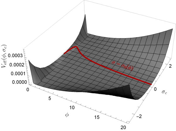
In figure 1 we display the two-field effective potential of Eq. (4.8) (for the canonical normalized pseudoscalar ) using the coupling functions (4.15)-(4.16) and the quartic potential . For illustrative purposes we have chosen a linear dependence on for the function , i.e. . The values of the rest of the parameters are66 6 The parameter will be set equal to one from now on without any further reference to it. It turns out that, along the minimum line, where we study inflation, it appears only on the higher order kinetic term which is negligible anyway. and . The parameter is fixed by the observed value of the amplitude of the scalar power spectrum, , at the pivot scale . The red curve corresponds to the minimum direction of Eq. (4.9). As it is evident from this figure, in the direction the potential grows exponentially as gets larger, hence the pseudoscalar is doomed to fall into the valley. This will be verified in the framework of the numerical treatment of the next section.
It is interesting to have a look at the resulting effective Lagrangian along the line in the large field limit. Taking the potential to be a standard renormalizable quartic potential , we obtain
| (4.17) |
The potential shows the familiar Palatini-plateau, while the kinetic term is expressed in terms of an effective -parameter
| (4.18) |
Note that is less than . We have not displayed in (4.17) the quartic kinetic term, anticipating that it is not expected to play any role in inflationary considerations, something that will be supported by our subsequent numerical analysis.
In figure 2 we have plotted the single-field effective potential results when the pseudoscalar moves along the minimum line , i.e. . The values of the parameters have been taken to be the same with those in figure 1. Since the inversion from the non-canonical field to the canonical one cannot be achieved analytically, we plot (blue dotted line) and (red line) doing the inversion to the canonical field numerically.
5 Inflation
In this section we analyze the inflationary behaviour of the model. We aim at restricting the parametric space, comparing its inflationary predictions to the corresponding latest observational bounds as set by the latest combination of Planck, BICEP/Keck and BAO data [14, 15].
5.1 Single-field inflation
Our system of two fields is described by the action (4.7), where the functions77 7 For simplicity we have omitted the arguments of these functions. and are given by (4.8). Starting from this action the equations of motion arising from it in an FRW background are88 8 Notice here that we use the canonical normalized pseudoscalar, given by Eq. (4.10).
| (5.1) |
where the total energy density and pressure are
| (5.2) |
We have considered the system of differential equations for and and solved it numerically. We start with indicative initial field values and zero velocities . The parameters are chosen at the characteristic values , and . The results are shown in figure 3. It is evident that when reaches the inflationary plateau, the has already fallen into the valley defined by the minimum line (4.9). This can be also understood by comparing the relevant mass of the field with the inflationary Hubble scale. After a numerical calculation we obtain that (for the benchmark case of figure 3) at times , which reinforces further the conclusion that the model is downgraded to a single-field inflationary model.
Therefore, for the inflationary period it would be sufficient to study the single-field problem described by . Then, the system is described by the single field action
| (5.3) |
where
| (5.4) |
Note that both kinetic functions and are positive definite.
Considering an FRW background, we obtain from (5.3) the following set of equations of motion
| (5.5) |
where the energy density and pressure are given by
| (5.6) |
Although we have displayed the single-field equations of motion for general , in the analysis of inflationary observables that will follow we have focused on , and .
Due to the appearance of the higher order kinetic term in the equation of motion the speed of sound in general deviates from unity. This can be easily seen from the form of the speed of sound which is given by
| (5.7) |
Nevertheless, the deviation from unity turns out to be quite small.
5.2 Inflationary observables
As it is quite complicated to find analytical expressions for the inflationary observables, we will solve the equation of motion (5.5) numerically to calculate them. To be as precise as possible the calculation of the amplitude of the scalar power spectrum , the spectral index , and the tensor-to-scalar ratio , is done in the framework of the adiabatic approximation as described in [72]. This method is suitable for theories with varying speed of sound and resembles to the well known WKB method. In our model even though the speed of sound is not constant, it is very close to unity throughout the full inflationary period, resulting to insignificant corrections to the inflationary observables.
Following [72], in order to calculate the observables we will use the Hubble flow functions given by
| (5.8) |
The scalar () and tensor () power spectra can be expanded around the arbitrary pivot scale , that exited the sound horizon at some time . keeping the first order terms in the Hubble flow functions (5.8), we obtain
| (5.9) | |||||
| (5.10) |
where the constant is given by . The corresponding amplitudes, for scalar and tensor perturbations, are given by,
| (5.11) |
The Planck 2018 data [14], yield a value for the amplitude of the scalar power spectrum , at the pivot scale .
The tensor-to-scalar ratio () and the spectral index of the scalar power spectrum () are given by
| (5.12) | |||||
| (5.13) |
The recent release of the BICEP/Keck [15] data, imposes the bound at the C.L. where the subscript denotes the pivot scale in . Furthermore, the combination of WMAP, Planck and BICEP/Keck data constrains the spectral index to the range again at the C.L. for .
After the end of inflation, the Universe enters to the radiation-dominated era through a reheating phase, which may last some folds or can be instantaneous. Following [73], we can compute the number of folds during inflation after the comoving scale, , crosses the sound horizon by defining , where denote the scale factor at the end of inflation and at the scale respectively. Analyzing the scale factor as
| (5.14) |
and assuming instantaneous reheating () and entropy conservation, we obtain
| (5.15) |
The subscripts “reh” and “0” denote evaluations at the end of reheating and present epoch respectively, while are the entropy density degrees of freedom being assuming the Standard Model particle content and temperatures or higher. Having in mind that , , 99 9 This equality is exact if there are no higher order kinetic terms. In [33] the higher-order kinetic terms have been taken into account, but as it is shown there, only an insignificant correction arises. and omitting the speed of sound contribution we obtain for the pivot scale that
| (5.16) |
At the pivot scale , in which the tensor-to-scalar ratio is calculated in some of our figures, the numerical coefficient increases to the value .
Let us now turn to the analysis of the parametric space of the model under consideration with respect to its predictions for the cosmological observables. For the parameter we choose to start from the value , since as discussed in [33] in the “simple” Palatini- model for values the spectral index can be within observational limits. It is also acceptable to use lower values, but at the price of reducing the range of acceptable e-folds considerably. For vanishing the spectral index and the tensor-to-scalar ratio are given approximately by
| (5.17) |
In our case both of them get modified, but their analytic expressions are not available since the functions involved are too complicated. We will examine two limiting cases for the function for the sake of better understanding of the behaviour of the observables.
In figure 4 we explore the case in which the linear part of the non-minimal coupling function of Eq. (4.16) dominates, taking the parameter to be zero. In this figure we show the predictions of the model in the direction using pivot scales for and for . For each given set of values for the parameters, we have employed Eq. (5.15) to obtain the number of -folds that complies with the constraints from reheating, while the value of quartic coupling is fixed by the observed value of the amplitude of the scalar power spectrum, , at the pivot scale . The parameter is fixed to the value , while (green dashed-dotted line), (red dashed line) and (black dotted line). The parameter varies from to in each curve in a clockwise direction as indicated in the figure. As the parameter gets larger the tensor-to-scalar ratio increases. The spectral index decreases up to some value of beyond which it starts to increase. A notable remark is that the predictions for and “freeze” to some values (their largest values) without being affected by a further increasing of the parameter . This “freezing” occurs at the values of and for and respectively, see also Table 2. In figure 5 we also present the observables versus the parameter , for better understanding of the analysis above.
In Figs. 6 and 7 we explore the case in which the cubic part of the non-minimal coupling function of Eq. (4.16) dominates, i.e. we choose . In this case the tensor-to-scalar ratio is constantly increasing as gets larger (from to ), while the spectral index initially increases, gets its maximum value and then starts to decrease and go well outside of the observational acceptable bounds [14, 15]. The datasets that correspond to the maximum value of are given in Table 3. The values of the rest parameters and the coloring of Figs. 6 and 7 are the same with that in Figs. 4 and 5.
In all of the figures presented the parameter has the value , but for any value lower than the predictions will remain unaffected. This can be easily understood if we have a look at the large field limits of the effective potential and the kinetic term (see Eq. (4.17)). For both of them the limits are functions of the combination , which means that if the inflationary predictions are controlled by . In the parameter space under consideration the ratio is always larger than . In particular, in Figs. 6-7 varies from (for ), (for ) and (for ). Similar values are noticed also in Figs. 4-5. At this point, we would like to mention that we do not consider larger values of that would drive us to the regime , since the tensor-to-scalar ratio would be even smaller. The sensitivity in the measurement of the tensor-to-scalar ratio by the next-generation CMB satellites [74, 75, 76] is expected to be , so smaller values for are only subject of academic significance. The general picture is that the presence of the pseudoscalar and its coupling to the inflaton through the term has as a result an increase of the tensor-to-scalar ratio, in comparison to the Palatini- model, while the spectral index can either decrease or increase depending on the rest of the parameters. In the whole range of the aforementioned parameters the number of -folds is calculated to be , under the assumption of instantaneous reheating. A smaller number of -folds can arise for larger values of , nevertheless, this would also lead to a smaller value for the tensor-to-scalar ratio.
6 Conclusions
In the present article we considered the framework of Metric-Affine theories of gravity in which the metric and the connection are independent variables. We extended the Einstein-Hilbert action to include the parity-odd Holst invariant as well as quadratic terms of it and of the Ricci scalar, expected to be generated by quantum corrections. This context gives rise to a new dynamical pseudoscalar degree of freedom. Furthermore, we considered the coupling of this system to a scalar field through the non-minimal terms and , the latter corresponding to a coupling of with the new pseudoscalar. The potential of the resulting Einstein-frame action of the two fields and has a minimum line along . Considering this model in an FRW background we found that the pseudoscalar falls quickly into the valley defined by the minimum line , this transition being supported by the numerical solution of the two-field system of equations of motion. Thus, the model is reduced to an effectively single-field model. Furthermore, along this minimum line the potential takes the form of the Palatini- potential with its characteristic inflationary plateau.
We have proceeded to study the resulting single-field inflationary model making a choice of the coupling functions and . A numerical calculation of the inflationary observables was undertaken in the framework of the adiabatic approximation [72]. The parametric space was constrained by the latest available bounds set by [14, 15]. We have found that our model complies with observations for a wide range of parameters. More precisely taking the parameter to be , the parameters and run in the range . We examined two limiting cases for the function in order to better understand the behaviour of the observables: the linear case () and the qubic case (). In the linear case the predictions for and “freeze” to their largest values without being affected by a further increase of the parameter . This “freezing” occurs at the values of and for and respectively. In the cubic case after the initial increase of the spectral index, once it gets its maximum value, it starts to decrease and go well outside of the observational acceptable bounds as gets larger. In general we found that the coupling has as a result an increase of the tensor-to-scalar ratio, in comparison to the Palatini- model, while the spectral index can either decrease or increase depending on the position in parametric space. The coefficient of the term does not modify the inflationary observables, while the one of the term can have a significant result only if it is larger than , which case is not considered here. Finally, under the assumption of instantaneous reheating, in the whole range of the aforementioned parameters the number of -folds measured from the end of inflation to the pivot scale is .
Summarizing, we have considered a general quadratic Metric-Affine theory, featuring an extra dynamical degree of freedom, and coupled it non-minimally to a scalar field. We studied inflation in the resulting two-field model and found that it effectively reduces to a single-field model, with a potential of the Palatini- form with its characteristic inflationary plateau and a modified kinetic term. We find that the inflationary predictions of this model fall within the latest observational bounds for a wide range of parameters. Furthermore, it allows for an increase in the tensor-to-scalar ratio.
Acknowledgments
The work of IDG was supported by the Estonian Research Council grant SJD18. KT would like to thank the CERN Theoretical Physics Department and the Laboratoire de Physique de l’Ecole Normale Superieure, where part of this work was done, for their hospitality.
References
- [1] A. A. Starobinsky, A New Type of Isotropic Cosmological Models Without Singularity, Phys. Lett. B 91 (1980) 99–102.
- [2] D. Kazanas, Dynamics of the Universe and Spontaneous Symmetry Breaking, Astrophys. J. Lett. 241 (1980) L59–L63.
- [3] K. Sato, First Order Phase Transition of a Vacuum and Expansion of the Universe, Mon. Not. Roy. Astron. Soc. 195 (1981) 467–479.
- [4] A. H. Guth, The Inflationary Universe: A Possible Solution to the Horizon and Flatness Problems, Phys. Rev. D 23 (1981) 347–356.
- [5] A. D. Linde, A New Inflationary Universe Scenario: A Possible Solution of the Horizon, Flatness, Homogeneity, Isotropy and Primordial Monopole Problems, Phys. Lett. B 108 (1982) 389–393.
- [6] A. Albrecht and P. J. Steinhardt, Cosmology for Grand Unified Theories with Radiatively Induced Symmetry Breaking, Phys. Rev. Lett. 48 (1982) 1220–1223.
- [7] A. D. Linde, Chaotic Inflation, Phys. Lett. B 129 (1983) 177–181.
- [8] A. A. Starobinsky, Spectrum of relict gravitational radiation and the early state of the universe, JETP Lett. 30 (1979) 682–685.
- [9] V. F. Mukhanov and G. V. Chibisov, Quantum Fluctuations and a Nonsingular Universe, JETP Lett. 33 (1981) 532–535.
- [10] S. W. Hawking, The Development of Irregularities in a Single Bubble Inflationary Universe, Phys. Lett. B 115 (1982) 295.
- [11] A. A. Starobinsky, Dynamics of Phase Transition in the New Inflationary Universe Scenario and Generation of Perturbations, Phys. Lett. B 117 (1982) 175–178.
- [12] A. H. Guth and S. Y. Pi, Fluctuations in the New Inflationary Universe, Phys. Rev. Lett. 49 (1982) 1110–1113.
- [13] J. M. Bardeen, P. J. Steinhardt, and M. S. Turner, Spontaneous Creation of Almost Scale - Free Density Perturbations in an Inflationary Universe, Phys. Rev. D 28 (1983) 679.
- [14] Planck Collaboration, Y. Akrami et al., Planck 2018 results. X. Constraints on inflation, Astron. Astrophys. 641 (2020) A10, [arXiv:1807.06211].
- [15] BICEP, Keck Collaboration, P. A. R. Ade et al., Improved Constraints on Primordial Gravitational Waves using Planck, WMAP, and BICEP/Keck Observations through the 2018 Observing Season, Phys. Rev. Lett. 127 (2021), no. 15 151301, [arXiv:2110.00483].
- [16] F. L. Bezrukov and M. Shaposhnikov, The Standard Model Higgs boson as the inflaton, Phys. Lett. B 659 (2008) 703–706, [arXiv:0710.3755].
- [17] A. Palatini, Deduzione invariantiva delle equazioni gravitazionali dal principio di Hamilton, Rend. Circ. Matem. Palermo 43 (1919) 203–212.
- [18] T. P. Sotiriou and S. Liberati, Metric-affine f(R) theories of gravity, Annals Phys. 322 (2007) 935–966, [gr-qc/0604006].
- [19] M. Borunda, B. Janssen, and M. Bastero-Gil, Palatini versus metric formulation in higher curvature gravity, JCAP 11 (2008) 008, [arXiv:0804.4440].
- [20] T. P. Sotiriou and V. Faraoni, f(R) Theories Of Gravity, Rev. Mod. Phys. 82 (2010) 451–497, [arXiv:0805.1726].
- [21] A. De Felice and S. Tsujikawa, f(R) theories, Living Rev. Rel. 13 (2010) 3, [arXiv:1002.4928].
- [22] G. J. Olmo, Palatini Approach to Modified Gravity: f(R) Theories and Beyond, Int. J. Mod. Phys. D 20 (2011) 413–462, [arXiv:1101.3864].
- [23] T. Clifton, P. G. Ferreira, A. Padilla, and C. Skordis, Modified Gravity and Cosmology, Phys. Rept. 513 (2012) 1–189, [arXiv:1106.2476].
- [24] S. Capozziello and M. De Laurentis, Extended Theories of Gravity, Phys. Rept. 509 (2011) 167–321, [arXiv:1108.6266].
- [25] F. Bauer and D. A. Demir, Inflation with Non-Minimal Coupling: Metric versus Palatini Formulations, Phys. Lett. B 665 (2008) 222–226, [arXiv:0803.2664].
- [26] V.-M. Enckell, K. Enqvist, S. Rasanen, and L.-P. Wahlman, Inflation with term in the Palatini formalism, JCAP 02 (2019) 022, [arXiv:1810.05536].
- [27] I. Antoniadis, A. Karam, A. Lykkas, and K. Tamvakis, Palatini inflation in models with an term, JCAP 11 (2018) 028, [arXiv:1810.10418].
- [28] F. Bombacigno and G. Montani, Big bounce cosmology for Palatini gravity with a Nieh–Yan term, Eur. Phys. J. C 79 (2019), no. 5 405, [arXiv:1809.07563].
- [29] I. Antoniadis, A. Karam, A. Lykkas, T. Pappas, and K. Tamvakis, Rescuing Quartic and Natural Inflation in the Palatini Formalism, JCAP 03 (2019) 005, [arXiv:1812.00847].
- [30] T. Tenkanen, Minimal Higgs inflation with an term in Palatini gravity, Phys. Rev. D 99 (2019), no. 6 063528, [arXiv:1901.01794].
- [31] A. Edery and Y. Nakayama, Palatini formulation of pure gravity yields Einstein gravity with no massless scalar, Phys. Rev. D 99 (2019), no. 12 124018, [arXiv:1902.07876].
- [32] T. Tenkanen, Trans-Planckian censorship, inflation, and dark matter, Phys. Rev. D 101 (2020), no. 6 063517, [arXiv:1910.00521].
- [33] I. D. Gialamas and A. Lahanas, Reheating in Palatini inflationary models, Phys. Rev. D 101 (2020), no. 8 084007, [arXiv:1911.11513].
- [34] T. Tenkanen and E. Tomberg, Initial conditions for plateau inflation: a case study, JCAP 04 (2020) 050, [arXiv:2002.02420].
- [35] A. Lloyd-Stubbs and J. McDonald, Sub-Planckian inflation in the Palatini formulation of gravity with an term, Phys. Rev. D 101 (2020), no. 12 123515, [arXiv:2002.08324].
- [36] I. Antoniadis, A. Lykkas, and K. Tamvakis, Constant-roll in the Palatini- models, JCAP 04 (2020), no. 04 033, [arXiv:2002.12681].
- [37] D. M. Ghilencea, Palatini quadratic gravity: spontaneous breaking of gauged scale symmetry and inflation, Eur. Phys. J. C 80 (4, 2020) 1147, [arXiv:2003.08516].
- [38] N. Das and S. Panda, Inflation and Reheating in f(R,h) theory formulated in the Palatini formalism, JCAP 05 (2021) 019, [arXiv:2005.14054].
- [39] Y. Tang and Y.-L. Wu, Weyl scaling invariant gravity for inflation and dark matter, Phys. Lett. B 809 (2020) 135716, [arXiv:2006.02811].
- [40] I. D. Gialamas, A. Karam, and A. Racioppi, Dynamically induced Planck scale and inflation in the Palatini formulation, JCAP 11 (2020) 014, [arXiv:2006.09124].
- [41] D. M. Ghilencea, Gauging scale symmetry and inflation: Weyl versus Palatini gravity, Eur. Phys. J. C 81 (2021), no. 6 510, [arXiv:2007.14733].
- [42] D. Iosifidis, A. C. Petkou, and C. G. Tsagas, Torsion/non-metricity duality in f(R) gravity, Gen. Rel. Grav. 51 (2019), no. 5 66, [arXiv:1810.06602].
- [43] D. Iosifidis and L. Ravera, Parity Violating Metric-Affine Gravity Theories, Class. Quant. Grav. 38 (2021), no. 11 115003, [arXiv:2009.03328].
- [44] S. Bekov, K. Myrzakulov, R. Myrzakulov, and D. S.-C. Gómez, General slow-roll inflation in gravity under the Palatini approach, Symmetry 12 (2020), no. 12 1958, [arXiv:2010.12360].
- [45] K. Dimopoulos and S. Sánchez López, Quintessential inflation in Palatini gravity, Phys. Rev. D 103 (2021), no. 4 043533, [arXiv:2012.06831].
- [46] A. Karam, E. Tomberg, and H. Veermäe, Tachyonic preheating in Palatini inflation, JCAP 06 (2021) 023, [arXiv:2102.02712].
- [47] A. Lykkas and K. Tamvakis, Extended interactions in the Palatini- inflation, JCAP 08 (2021), no. 043 [arXiv:2103.10136].
- [48] D. Sáez-Chillón Gómez, 3+1 decomposition in modified gravities within the Palatini formalism and some applications, arXiv:2103.16319.
- [49] I. D. Gialamas, A. Karam, T. D. Pappas, and V. C. Spanos, Scale-invariant quadratic gravity and inflation in the Palatini formalism, Phys. Rev. D 104 (2021), no. 2 023521, [arXiv:2104.04550].
- [50] I. Antoniadis, A. Guillen, and K. Tamvakis, Ultraviolet behaviour of Higgs inflation models, JHEP 08 (2021) 018, [arXiv:2106.09390]. [Addendum: JHEP 05, 074 (2022)].
- [51] J. Annala and S. Rasanen, Inflation with terms in the Palatini formulation, JCAP 09 (2021) 032, [arXiv:2106.12422].
- [52] C. Dioguardi, A. Racioppi, and E. Tomberg, Slow-roll inflation in Palatini F(R) gravity, JHEP 06 (2022) 106, [arXiv:2112.12149].
- [53] M. AlHallak, N. Chamoun, and M. S. Eldaher, Natural Inflation with non minimal coupling to gravity in R 2 gravity under the Palatini formalism, JCAP 10 (2022) 001, [arXiv:2202.01002].
- [54] K. Dimopoulos, A. Karam, S. Sánchez López, and E. Tomberg, Modelling Quintessential Inflation in Palatini-Modified Gravity, Galaxies 10 (2022), no. 2 57, [arXiv:2203.05424].
- [55] S. Panda, A. A. Tinwala, and A. Vidyarthi, Ultraviolet Unitarity Violations in Higgs’-Coupled Starobinsky Inflation, arXiv:2205.12836.
- [56] K. Dimopoulos, A. Karam, S. Sánchez López, and E. Tomberg, Palatini R 2 quintessential inflation, JCAP 10 (2022) 076, [arXiv:2206.14117].
- [57] R. Durrer, O. Sobol, and S. Vilchinskii, Magnetogenesis in Higgs-Starobinsky inflation, arXiv:2207.05030.
- [58] I. Antoniadis, A. Guillen, and K. Tamvakis, Late time acceleration in Palatini gravity, JHEP 11 (2022) 144, [arXiv:2207.13732].
- [59] A. B. Lahanas, Issues in Palatini inflation: Bounds on the Reheating Temperature, arXiv:2210.00837.
- [60] S. Panda, A. Rana, and R. Thakur, Constant-Roll Inflation in modified gravity model using Palatini Formalism, arXiv:2212.00472.
- [61] A. Baldazzi, O. Melichev, and R. Percacci, Metric-Affine Gravity as an effective field theory, Annals Phys. 438 (2022) 168757, [arXiv:2112.10193].
- [62] F. W. Hehl, J. D. McCrea, E. W. Mielke, and Y. Ne’eman, Metric affine gauge theory of gravity: Field equations, Noether identities, world spinors, and breaking of dilation invariance, Phys. Rept. 258 (1995) 1–171, [gr-qc/9402012].
- [63] G. Pradisi and A. Salvio, (In)equivalence of metric-affine and metric effective field theories, Eur. Phys. J. C 82 (2022), no. 9 840, [arXiv:2206.15041].
- [64] A. Salvio, Inflating and reheating the Universe with an independent affine connection, Phys. Rev. D 106 (2022), no. 10 103510, [arXiv:2207.08830].
- [65] R. Hojman, C. Mukku, and W. A. Sayed, PARITY VIOLATION IN METRIC TORSION THEORIES OF GRAVITATION, Phys. Rev. D 22 (1980) 1915–1921.
- [66] S. Holst, Barbero’s Hamiltonian derived from a generalized Hilbert-Palatini action, Phys. Rev. D 53 (1996) 5966–5969, [gr-qc/9511026].
- [67] G. Immirzi, Quantum gravity and Regge calculus, Nucl. Phys. B Proc. Suppl. 57 (1997) 65–72, [gr-qc/9701052].
- [68] G. Immirzi, Real and complex connections for canonical gravity, Class. Quant. Grav. 14 (1997) L177–L181, [gr-qc/9612030].
- [69] C. Rigouzzo and S. Zell, Coupling metric-affine gravity to a Higgs-like scalar field, Phys. Rev. D 106 (2022), no. 2 024015, [arXiv:2204.03003].
- [70] M. Langvik, J.-M. Ojanperä, S. Raatikainen, and S. Räsänen, Higgs inflation with the Holst and the Nieh–Yan term, Phys. Rev. D 103 (2021), no. 8 083514, [arXiv:2007.12595].
- [71] M. Shaposhnikov, A. Shkerin, I. Timiryasov, and S. Zell, Higgs inflation in Einstein-Cartan gravity, JCAP 02 (2021) 008, [arXiv:2007.14978].
- [72] J. Martin, C. Ringeval, and V. Vennin, K-inflationary Power Spectra at Second Order, JCAP 06 (2013) 021, [arXiv:1303.2120].
- [73] A. R. Liddle and S. M. Leach, How long before the end of inflation were observable perturbations produced?, Phys. Rev. D 68 (2003) 103503, [astro-ph/0305263].
- [74] T. Matsumura et al., Litebird: Mission overview and focal plane layout, Journal of Low Temperature Physics 184 (Aug, 2016) 824–831.
- [75] A. Kogut, D. Fixsen, D. Chuss, J. Dotson, E. Dwek, M. Halpern, G. Hinshaw, S. Meyer, S. Moseley, M. Seiffert, D. Spergel, and E. Wollack, The primordial inflation explorer (PIXIE): a nulling polarimeter for cosmic microwave background observations, Journal of Cosmology and Astroparticle Physics 2011 (jul, 2011) 025–025.
- [76] NASA PICO Collaboration, S. Hanany et al., PICO: Probe of Inflation and Cosmic Origins, arXiv:1902.10541.