Detecting causal covariates for extreme dependence structures
2Institute of Mathematics, École polytechnique fédérale de Lausanne, Switzerland
Abstract
Determining the causes of extreme events is a fundamental question in many scientific fields. An important aspect when modelling multivariate extremes is the tail dependence. In application, the extreme dependence structure may significantly depend on covariates. As for the general case of modelling including covariates, only some of the covariates are causal. In this paper, we propose a methodology to discover the causal covariates explaining the tail dependence structure between two variables. The proposed methodology for discovering causal variables is based on comparing observations from different environments or perturbations. It is a desired methodology for predicting extremal behaviour in a new, unobserved environment. The methodology is applied to a dataset of concentration in the UK. Extreme levels can cause severe health problems, and understanding the behaviour of concurrent severe levels is an important question. We focus on revealing causal predictors for the dependence between extreme observations at different sites.
Introduction
Modelling extreme events is a crucial part of many real-world problems and the focus is often on the extremal dependence structure between several variables (Coles 2001). In a univariate case, under very general assumptions, a normalized maxima of random variables converges to a Generalized Extreme Value (GEV) distribution (Gnedenko 1943). In the multivariate case, however, the limiting dependence structures for extreme values do not follow a simple parametric form. Therefore, alternative joint tail representations should be used, and extensive literature describes different approaches (Resnick 1987; Beirlant et al. 2006).
More recent literature describes the modelling and estimation of covariate influence on the joint tail structure. Mhalla et al. 2019b propose a parametric framework for integrating covariate information through the angular density model. Non-parametric modelling of the joint tail structure using GAM modelling (Wood 2017) has been developed in Mhalla et al. 2017. In this paper, our main emphasis is on the causal properties of the extremal tail coefficient between two random variables (Joe 1997).
A real-world problem of interest consists of measurements in the UK. Features of concentration levels or other air pollutants are of interest in environmental science (Shi et al. 2014) as extreme values of can be very dangerous and have been linked to an increased risk of lung cancer (Hamra et al. 2018). The dataset taken from Carslaw and Ropkins 2022 comprises 241 measurement stations in the UK with hourly records of [µg/m3]. We use only the stations with at least 15 years of measurements (21 stations in total). is partially produced by burning fossil fuel and motor vehicle exhaust. Hence, we distinguish traffic stations where the level is predominantly determined by nearby traffic (12 stations) from background stations (9 stations). Figure 1 shows concentration (in g/m3) for one traffic station and one background station over time. We observe that the magnitude is usually larger in traffic stations than in background stations. Although a yearly seasonality seems clearer for the background station, both series highlight a long term decreasing trend. The point of our interest is the extremal dependence between a pair of stations explained by some covariates. Some of these covariates may be causal, others not. We are interested in answering the following question: What is the cause of the extremal dependence between concentrations at two stations?

Determining a system’s causal structure is an important problem in many scientific fields. There is a growing literature on causal inference under various types of assumptions and different frameworks, with applications ranging from public health to biology and economics (Chang et al. 2015; Varian 2016). Often, the goal is to find the causes of some response variable among a given set of covariates X or to quantify the causal relationships between a set of variables. In recent years, a causal discovery based on conditional invariance has become an important growing research area. Starting with a groundwork paper (Peters et al. 2016), connections between distributional invariance and causality started to emerge. The reviewing paper Bühlmann 2020 summarises the groundwork and highlights the importance of causal prediction. The methodology based on invariant causal prediction (ICP) relies on observing a system under different environments (Pearl 2009). Then, one can observe some invariant properties for causal variables through all environments, but not for non-causal ones.
Here, we are interested in unveiling causal links explaining extremal dependence between random variables. Precisely, we want to assess whether an intervention on a covariate affects the tail dependence of the random variables. Classical causal techniques that usually give a good description of data tend to fail in the upper tail due to the scarcity of observations (Engelke and Ivanovs 2021). A combination of causality and extreme value theory (EVT) is a developing research area. Mhalla et al. 2019a use a Kolmogorov complexity to detect causal direction using observational data. Kiriliouk and Naveau 2020 studied probabilities of necessary and sufficient causation as defined in the counterfactual theory using the multivariate generalized Pareto distributions. Gnecco et al. 2020 define a causal tail coefficient revealing the causal structure between two random variables by capturing asymmetries in the extremal dependence of the two random variables under the context of the linear structural causal model. Their methodology holds also in the presence of latent common causes with the same tail heaviness as the observed variables. Pasche et al. 2021 proposes a methodology relying on the causal tail coefficient that can deal with latent common causes that have different tail indices. Deuber et al. 2021 describe a framework for estimating extremal quantile treatment effects. However, to our knowledge, no theory combines EVT and causal inference using the ICP framework and inferring causes of the extremal dependence structure.
A well-established approach in causal inference relies on the structural causal model (SCM) of Pearl 2009. The ICP framework exploits invariance properties in SCM for inference; see Haavelmo 1944; Dawid 2006; Schölkopf et al. 2012 for similar notions. The main emphasis in the ICP setting has been on linear regression models assuming the additive form , where is the response variable of interest, is the set of direct causal covariates among the set of covariates X and the set of indices of direct causes of . Generalizations of this model have been given by Heinze-Deml et al. 2018 with the more flexible form where is a smooth, non-parametric function. We aim to use the ICP methodology in the context of the joint tail structure.
The paper is organized as follows: Section 1 introduces EVT in the bivariate context. Section 2 describes the ICP methodology. Section 3 proposes a methodology to unveil causal covariates among a set of covariates explaining the extremal dependence between two random variables. A simulation study is presented in Section 4 and Section 5 illustrates the proposed methodology through the dataset of measurements in the UK.
1 Bivariate extreme value theory
Let be a sequence of independent and identically distributed (iid) random variables with common distribution . We are interested in the behaviour of the maximum of a sequence of such random variables, that is . If there exist a non-degenerate distribution and sequences of constants and such that as , then belongs to the Generalized Extreme Value (GEV) distributions family. The GEV distribution has three parameters, namely a location , a scale , and a shape . Its distribution function takes the form
| (1) | ||||
defined on the support for cases respectively. Cases when , and correspond to the Fréchet, Gumbel, and Weibull distributions, respectively (Fisher and Tippett 1928; Gnedenko 1943).
Suppose now is a sequence of independent copies of a two dimensional random vector with marginal distributions , and joint distribution and denote by their component-wise maxima. We suppose that there exist sequences and such that the normalized vector converges in distribution to a random vector Z with joint distribution and non-degenerate margins , . Then, the limiting distribution is called the multivariate extreme value distribution (MEVD) (Resnick 1987, Chapter 5.3). The class of MEVDs coincides with the class of max-stable distribution functions with non-degenerate margins. The margins are max-stable, or equivalently GEV. Without loss of generality, it is convenient to transform the marginal distributions to unit Fréchet margins with distribution function . The transformation is marginally performed using a probability integral transform with
| (2) |
applied to the th GEV margin . When the margins are transformed to unit Fréchet, the dependence structure of the transformed random vector is the same as the dependence structure of the vector Z. We therefore assume hereafter that Z has unit Fréchet margins. In that case, is called a simple max-stable distribution and has the representation , where is called the exponent function (Resnick 1987, Chapter 5.4). It can be shown that is homogeneous, that is, (Coles and Tawn 1991). The Pickands dependence function (Pickands 1981) is defined by
| (3) |
where is the unit simplex and , for any norm . The Pickands dependence function is the restriction of the exponent function to , and it measures the strength of extremal dependence along a direction . This function must satisfy the boundary restrictions where the lower bound corresponds to perfect extremal dependence and the upper bound to the independence case. It also satisfies the border conditions and is a continuous and convex function on . The extremal coefficient (Smith 1990), defined by
| (4) |
is a summary of the strength of extremal dependence between and . Noting that , the extremal coefficient lies between 1 (perfect dependence) and 2 (independence). Moreover,
| (5) |
In the rest of the paper, we focus mainly on modelling .
For modelling , it is common to use parametric representations of the exponent function . An example is the logistic model, defined as
| (6) |
Independence and complete dependence correspond to , , respectively (Tawn 1988). It is a symmetric model, where are exchangeable and a simple relation holds. Another example is the Hüsler–Reiss model, defined as
| (7) |
where is a Gaussian distribution function and is a parameter. Independence and complete dependence correspond to , , respectively, and holds (Engelke et al. 2015). Other commonly used parametric models include, for example, Dirichlet models (Tawn 1990).
In many applications, the extremal dependence structure depends on covariates. Consider the bivariate max-stable random vector given a set of observed covariates and suppose that it has unit Fréchet marginal distributions. Both the related Pickands function and extremal coefficient are therefore covariate-dependent and can be written for and . While our emphasis is on non-stationary extremal dependence structures, one may also consider the margins of to be covariate-dependent, that is, for . In that case, a regression model applied to the marginal GEV distributions’ parameters (Pauli and Coles 2001) is required to transform the margins to a unit Fréchet scale.
In order to infer about the covariate-dependent Pickands function, Mhalla et al. 2017 introduced, for a fixed direction in the unit simplex, the max-projection
where , and . It was shown that the resulting random variable is Beta distributed with parameters and . Hence, for a fixed value of , statistical inference for can be performed through likelihood procedures or regression techniques.
2 Causal modelling
First, we introduce a graphical causal notation (e.g., Spirtes et al. 2001). A DAG (directed acyclic graph) contains a finite set of vertices (nodes) and a set of directed edges between distinct vertices. We assume that there exist no directed cycle or multiple edges. Let be two distinct nodes of . We say that is a parent of if there exist an edge from to in , and denote . We usually omit in the notation if it is clear from context. Consider a random vector over a probability space . With a slight abuse of notation, we identify the vertices with the variables . We denote for . Typically, we denote , where (usually denoted by ) is a variable of interest and are covariates. We assume that follow a structural causal model (SCM) (Pearl 2009), defined as follows.
Definition 1.
The random variables (where plays the role of the target variable ) follow a SCM with DAG representing the causal structure (Verma and Pearl 2013) if for each the variable arises from a structural equation
where are jointly independent random variables. The functions are the assignments (or link functions) and we say that is a direct cause of , if .
We are interested in estimating the set of direct causes of . Doing that only from a random sample is often impossible, unless we assume some identifiable structure and additional strong assumptions (Shimizu et al. 2006; Peters et al. 2014).
Definition 2 (Intervention).
Consider an SCM as in Definition 1. We replace one of the structural equations to obtain a new SCM. Assume that we replace the assignment for by , where the new is independent of all and are potentially arbitrary. We then call the entailed distribution of the new SCM an intervention distribution and say that has been intervened on.
A classical example of an intervention is a hard (atomic) intervention on (Peters et al. 2017, Definition 6.8.), replacing the structural equation in the SCM by . Note the difference between a simple conditioning and a hard intervention, where we assume that the joint distribution results from a different data-generating process.
More generally, suppose that we observe in different environments (Peters et al. 2017, Section 7.1.6). In each environment , there is a target variable and covariates . The number of environments is assumed finite. The set of environments is defined in a general way by assuming that for each , follows (a different) SCM with distribution . A different environment can be generated by (possibly several) interventions (Eberhardt and Scheines 2007) on the covariates. However, we do not assume that any information about the interventions is known.
Note that interventions on X do not change the conditional distribution of . We assume that the parents of remain the same in all environments. Consider the set of indices determining the covariates of X that are true direct causes of . Invariance based causal discovery (Peters et al. 2016) relies on the fact that is invariant for each . We can put it more formally by assuming the following:
Assumption 1.
There exist , a function and a distribution , such that for all we have
| (8) |
In other words, the structural equation for the target variable can be written as for all . The link function remains the same in all environments, and noise variables are iid. As discussed in Bühlmann 2020, Assumption 1 guarantees that on one hand does not change the mechanism between and , and on the other hand that does not act directly on and ideally, should change the distribution of .
In what follows, the formulation “Assumption 1 is valid for set ”, means that there exist and such that (8) holds with set . It is important to observe the following (Peters et al. 2016, Section 6.1):
Lemma 1.
Assumption 1 is valid for the set S if and only if for all we have for all x.
The ICP methodology stems from testing for each the following hypothesis:
Therefore,
| (9) |
is the proposed estimator of the set of direct causes .
If Assumption 1 holds and we have a proper test for , then will not be rejected on a given confidence level, and therefore . On the other hand, if we want to guarantee , we need to observe “enough” environments. It is a big challenge to show some necessary and sufficient conditions for the full identifiability of the causal variables. Some results are known in only special cases (Pfister and Peters 2022). It is easy to see that the more environments we observe, the larger is.
As for testing , we need to assume some form of the link function . Usually, classical regression methods are used to infer about the link function and testing is performed through a testing procedure such as a -sample test. However, if we have a test having a proper level , the Theorem 1 guarantees that each element of indeed lies in with probability .
Theorem 1.
(Peters et al. 2016) Let Assumption 1 be valid. Consider a test that has a level for . Then, the previously defined estimate fulfills
Hence, a proper test that has a level (at least asymptotically) is needed. One of the goals of the work by Heinze-Deml et al. 2018 was to conduct an appropriate test under different assumptions on the link function. Here, we use the invariant residual distribution test explained below.
2.1 Invariant residual distribution test
We assume that the link function from Assumption 1 is additive, that is, the structural equation is of the form
for all . The core of the proposed test for has two main steps:
- 1.
Pool the data together from all environments and fit a model to predict from . Stated differently, estimate relying on data from all environments.
- 2.
Use a -sample test to assess whether the residuals obtained from different environments have the same distribution.
A more detailed description can be found in Appendix II.5 in Heinze-Deml et al. 2018.
3 Causal modelling of extremal dependence
In order to frame the modelling of extremes into a structural causal setup, we start by introducing the LogMax-projection.
Lemma 2.
Assume that is a bivariate simple max-stable random vector with a Pickands dependence function and extremal coefficient . Denote . Let
where is the Euler constant. Then,
- •
is exponentially distributed with parameter . In particular, .
- •
, where 11 1 distribution function has the form . Specifically, ) is a centered Gumbel distribution.. In particular, .
Proof.
From and , we get
Similar results can be found in Mhalla et al. 2017 using the beta distribution. The results for follow easily when connecting . We use the fact that the minus logarithm of an exponential distribution is a Gumbel distribution and . The mean of the standard Gumbel distribution is , so we obtain centred Gumbel noise by subtracting . ∎
We will refer to defined in Lemma 2 as a LogMax-projection. This transformation is very useful when the interest is to make inference on . This can be done for instance through classical regression tools. More importantly, it has the desired property that the noise acts additively. Hence, it can be fitted into the causal framework of Heinze-Deml et al. 2018.
Remark 1.
Lemma 2 can be used to model the behaviour of the Pickands dependence function evaluated at the specific value . Arguably, this value is the most important in most applications due to its interpretability and connections to the tail dependence measures such as (5). However, we can easily modify Lemma 2 for any value , , by taking .
3.1 Covariate-dependent structures and GAM
Let us move now to the case where the extremal coefficient depends on a set of covariates . Consider a bivariate simple max-stable random vector with a covariate-dependent extremal coefficient. For any , we denote by , the extremal coefficient between conditioned on .
From Lemma 2, we have that the LogMax-projection is defined as
and satisfies
As mentioned above, one can use this model formulation to make inference on . We propose using the flexible generalized additive model (GAM) (Wood 2017) for the estimation of . Under the GAM framework, we make the following assumptions:
Assumption 2.
Let , where:
- •
is a link function,
- •
and are subsets of x, and
- •
are functions admitting a finite quadratic penalty representation (Green and Silverman 1994) supported on a closed set for all .
Note that in application, ignoring the fact that the extremal coefficient lies in and considering that it is real-valued instead, has no impact on the set of causal covariates discovery. For instance, we do not aim to estimate the extremal coefficient, per se, but rather compare the effect of the covariates under different environments. This does not affect the consistency. The estimation of is based on maximizing the penalized log likelihood:
| (10) |
where represents the set of unknown parameters ( and the linear basis coefficients of each of the smooth functions ) and is the log likelihood associated with the Gumbel observations , that is, . The integrated square second derivative penalties prevent interpolating estimate functions of and the smoothing parameters control the trade-off between model goodness of fit and model smoothness. When the estimate of tends to be a straight line.
The minimization of (10) is performed based on an outer-iteration procedure. At each iteration, and are estimated separately by penalized iteratively re-weighted least squares and a prediction error method from generalized cross validation, respectively (for details, see Chapter 5 in Wood 2017). Under appropriate regularity assumptions on the functions and the smoothing parameters, the GAM resulting estimator is consistent and asymptotically normal (Yoshida and Naito 2012; Wood 2017). More GAM-related theory is available, for example, in Wood et al. 2016.
3.2 LogMax-projection in SCM
Let us move to the causal setup. We assume that we observe variables from different environments , with the number of environments being finite. In environment , let be our covariates, be a simple max-stable random vector with covariate-dependent extremal coefficient . Let be the corresponding LogMax-projection in environment . In each environment, we observe iid observations . For , we denote the extremal coefficient between conditioned on (as a reminder, we denote for a set ).
Combining Assumption 1 and Lemma 2, we assume that the structural equation is of the form
where is the true set of parents. The following proposition states that the residuals are asymptotically invariant.
Proposition 1.
Suppose Assumption 1 holds. Let be an estimator of that is consistent in the sense that for all . Define the residuals . Take . Then, as the number of data (in both environments) tends to infinity, we have .
The proof is based on the fact that from Assumption 1 and that the estimator is consistent. Hence, the invariant residual distribution test (2.1) can be directly used. Note that Proposition 1 is formulated only for the set of true direct causes .
We can directly test the invariance property for all . This invariance should hold for the true set and hence, the same argument as in Theorem 1 can be used. In the following, we propose a methodology for testing this invariance property.
3.3 Generic algorithm
The proposed methodology can be summarized in the following algorithm.
- 1.
For each margin separately:
- •
Transform original data to unit Fréchet scale. This can be done by using the block maxima approach to fit a GEV distribution to the univariate series.
- •
The GEV parameters can also depend on other covariates.
- •
- 2.
In each environment separately:
- •
Compute the LogMax-projection ,
- •
- 3.
For each :
- •
Pool the data from all environments and calculate ,
- •
Compute the residuals ,
- •
Use a -sample test, to test if the residuals from different environments are equally distributed.
- •
- 4.
Get as the intersection of the subsets where the -sample test was not rejected.
In practice, we do not have to repeat the algorithm for all ; if we do not reject the -sample test for a set , testing for a superset of , is redundant.
Several approaches can be used for transforming the data to unit Fréchet margins. In our application, we fit a covariate-dependent GEV distribution to block maxima. Alternatively, a peak over threshold approach (Pickands 1975) can be used as well.
In our application, we use GAM to estimate based on minimizing (10). This choice was also used in Mhalla et al. 2017 and is a default method in non-linear ICP methodology in Heinze-Deml et al. 2018.
As for the -sample test, we use the Anderson-Darling -sample test (AD-test). In dimension two, the distance between the two samples is
where is an empirical distribution function of the pooled datasets. The -sample AD-test is the natural generalization of its two-sample counterpart (Scholz and Stephens 1987). It has typically better power than the Kolmogorov-Smirnov test (Razali and Yap 2011). This test is used at a level level. Note that an estimation error can arise from two sources: from the estimation of the margins, and from the estimation of . Although the equality should asymptotically hold, we do not claim that a proper level holds for a finite number of observations. In the following, we illustrate the methodology on a series of simulations.
4 Simulations
We proceed with a simulation study. Section 4.1 describes the study and results based on a specific example, discussing power with different causal strength, intervention strength and multicollinearity. Section 4.2 discusses a hidden confounder case, when Assumption 1 is not fulfilled. Section 4.3 deals with a case when we start with non-extreme data; we compare the choices of different thresholds and different marginal transformations and we discuss a case when we do not “clean the margins” properly.
We want to stress that we are only interested in inferring causal relations, not an inference on the extremal dependence structure itself.
4.1 Intervention, causal strength, and multicollinearity
Let have a simple bivariate max-stable distribution and be a set of covariates. We assume the distribution of to be parameterized by a logistic copula (6) with parameter . Since is a function of only, the true set of direct causes of our extremal dependence is therefore . We consider as other covariates, graphically represented by a SCM in the form , where is the LogMax-projection. We observe the covariates and the change of environments are interventions on , and . Details about the generation of the random variables can be found in Table 1 and the three parameters , and are as follows
- •
the parameter describes the strength of intervention. If then there is no intervention on ,
- •
the parameter represents the causal strength of on . If then is independent of ,
- •
the parameter describes the dependence between and . If then . Moreover, if , the correlation and if then .
We proceed with our causal methodology using the algorithm described in Section 3.3. We use repetitions for different choices of and for two sample sizes and . Figure 2 describes how often we get using our methodology. The upper axis in Figure 2 represents the expectation in the second environment under the corresponding intervention strength (note that in the first environment). Obviously, the larger the intervention , the higher the heterogeneity between the environments and hence the easier it is to find the correct causal set. The reason why we obtain worse results with a larger absolute value is that it becomes statistically harder to distinguish between correlated since both are good predictors (with an exception in the third environment). Not surprisingly, the larger the causal strength , the better the results we obtain.
| First environment | Second environment |
|---|---|
| , where | , where |
| where | where |
| , where | , where |
| Third environment | Fourth environment |
| , where | , where |
| where | |
| , where | , where |
4.2 Hidden confounder
We present a situation in which a hidden confounder of a causal covariate and the extremal dependence coefficient are present. The graphical representation of the model can be found in Figure 3.

Let have a simple bivariate max-stable distribution, are the observed covariates and is an unobserved covariate. We assume the distribution of to be parameterized by a Hüsler–Reiss copula (7) with parameter .
We intervene on and generate the variables in the corresponding environments:
- 1.
, where ,
- 2.
, , where .
Moreover, in both environments, we compute the LogMax-projection .
Finally, we compute based on only. Note that the only observed direct cause of is . However, due to the hidden variable , Assumption 1 no longer holds. It is easy to see that is invariant through environments, however, is not due to the hidden confounder. Simulations show how much this heuristic is justified in practice.
For a range of sample sizes , we generate the variables as described above, compute and repeat times. The results are described in Figure 4. We can see that for smaller , we tend to not reject for both . Hence, the resulting estimate is an empty set (intersection of ). For a larger , the test can recognise the effect of the hidden confounder and we tend to reject for , and hence, the resulting estimate is .
Note that if the effect of is small, we tend to accept for and also for which results in . On the other hand, if the effect of is large (larger than the effect of intervention), then the effect of on will be (proportionally) small and we tend to accept for . The statistical guarantees such as Theorem 1 or Theorem 1 for are no longer valid. However, following (Peters et al. 2016)[Proposition 5], will estimate some subset of its ancestors (instead of parents). For a more detailed discussion of hidden confounders in the non-extremal case, see (Peters et al. 2016)[Appendix C].
4.3 Effect on the margins
In this section, we consider the case when the observed covariate has an effect on the margins as well as on the dependence structure. Suppose we observe two covariates , where has an effect on the extremal dependence of and has an effect on the margins and . The graphical representation can be seen in Figure 5.

We simulate the following data: for , we consider are bivariate iid random variables distributed as a generic element , where margins , where for a parameter . The dependence structure between is modeled by a logistic copula with parameter . Hence, the dependence structure (as well as the extremal dependence structure) is a function of only.
We transform into a period-maxima, that is, we define
where the maxima is component-wise maxima.
Hence, we obtain independent maxima . We model their margins by a GEV distribution with parameters depending on . By fitting the covariate-dependent GEV distribution, we transform the margins into unit Frechet using (2). We model GEV parameters
and estimate them smoothly using the GAM framework. Finally, we compute the LogMax-projections .
We intervene on the covariates and observe the system. More precisely, we generate the variables in the corresponding environments as follows:
- 1.
, where ,
- 2.
, where ,
- 3.
, .
We consider the copula parameter in the form . In both environments, we generate and compute the LogMax-projections as mentioned before.
Finally, we estimate the set of direct causes of the extremal dependence structure following points 3 and 4 in Section 3.3. We repeat times for a range of parameters , and , where represents the effect of on the margins, is the size of the final dataset (of extremes) and is a size of the block maxima we take. The blue lines in Figure 6 represent the ratio of correctly estimating .
Now, consider a different question: What happens if we do not include for the marginal modelling? We proceed with the same setup as before, but we model GEV parameters and estimate them using maximum likelihood.
Again, we estimate the set of direct causes of the extremal dependence structure following points 3 and 4 in Section 3.3. We repeat times for a range of parameters , and . The red lines in Figure 6 represent the ratio of correctly estimating .
We can see that ignoring the marginal effects of creates a spurious causal effect on the extremal dependence structure. Indeed, if is large, the margins of Z tend to be both very large. Hence, extremes occur concurrently even though has no effect on the extremal copula, and our results are compromised.
The same holds if is hidden; if there exists a hidden covariate that affects both margins with “enough” strength, it can affect the inference about the extremal dependence structure. Therefore, it is good practice to include as many relevant covariates for the marginal inference as possible.
5 NO2 Application
We illustrate the causal methodology for the tail dependence on a dataset of concentration levels measured in the UK (Carslaw and Ropkins 2022). To explain the extremal coefficient between the levels of two different stations, we consider three different potential causal covariates . Namely, the distance (in kilometres) between the stations, the time (year) of the observation, and the type of area (traffic/non-traffic). A similar dataset is studied in Mhalla et al. 2019c. We wonder which of these covariates have a causal effect on the tail dependence. The choice of the time as a covariate may sound unusual as we expect that the physical mechanism is inherently given by laws of nature and does not change over time. However, it might be considered as a proxy for potential confounders such as the increase in temperature or .
5.1 Transforming margins and LogMax-projecting
We follow steps 1 and 2 from the algorithm (3.3). We transform our observations into bivariate simple max-stable ones. The first step is therefore transforming the margins to the unit Fréchet scale using transformation (2). We use weekly maxima (around 900 weeks at each station; recall that we have hourly measurements) and model these weekly maxima by a GEV distribution (1) with time-varying parameters
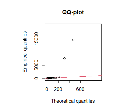
where represents the year and represents the week of the year, and are smooth functions. Inference is performed under the GAM framework (Youngman 2020) and likelihood ratio tests are conducted to assess whether we need smoothly varying terms or whether parametric and sinusoidal terms already provide a good fit. The final fitted model is then used to transform the data at each station to the unit Fréchet distribution using the probability integral transform (2). Figure 7 shows a QQ-plot of the resulting transformed observations for one of the stations (RBKC Chelsea in London) against the unit Fréchet. It shows a reasonable fit besides a few outliers.
The next step of the algorithm (3.3) is to pair the stations and compute the LogMax-projection. We pair only the stations with the same traffic type. We end up with 106 pairs of stations. For each pair, we compute the LogMax-projection transformation described in Lemma 2.
5.2 Defining environments
In this application, we define one environment as one pair of stations. Consider two pairs of stations for which all covariates remain unchanged, but changes from non-traffic to traffic. This can be considered as a "do-intervention" on the covariate since we assume that the underlying physical mechanism is the same regardless of the location of our stations. A few remarks on the choice of such environments are in order.
Remark 2.
Notice that this is not simple conditioning on traffic/non-traffic stations. Take measurements from one pair of stations. Imagine that we conduct an experiment where we artificially add traffic to those stations to see if the extremal coefficient changes. Instead of adding traffic to one station, we measure a second (different) pair that has the same value of covariates, except for traffic. The main difference here is that we assume that the data-generating process remains unchanged, apart from the traffic covariate.
Remark 3 (Possible hidden variable).
The main drawback is the following: Is there a hidden variable that differs between the pairs and causally affects our response? This is represented in Figure 8. We need to assume that there is no such variable or if there is, it has a negligible impact on the response variable.

Remark 4 (Time).
Each station is measured over a different period. Some stations started in 2003, some in 1997. For each pair, we take only the intersection of measured weeks. Hence, we can argue that by changing the pair, we also change the period of observations. However, this change is minor and almost negligible. Our findings support the fact that time is not a causal covariate. This might of course be due to changes between environments not being strong enough to find such evidence.
5.3 Details for the choices of environments and results for one choice of stations
We take five different environments, that is, five pairs of stations (10 different stations in total). We want the interventions to be “strong”. For , we choose one pair from each of the bins of distances described in Table 2. As for , we choose three pairs with the type traffic and two with the type non-traffic. In order to make an intervention on , we would need to divide the dataset into different periods and compare them. However, due to the limited time span of our dataset, this is not an option, so we cannot intervene on .
| <10km | (10km, 20km) | (20km, 50km) | (50km, 100km) | 100km< |
We explain now the results on one specific choice for the environments. This choice is described in Table 3. In Section 5.4, we repeat the experiments with 50 different choices to get more robust results. We estimate using the methodology described in Section 3.3. For each we test the invariance property using step 3 in algorithm 3.3. Results (for the specific choice of environments described in Table 3) are described in Table 4. The hypotheses corresponding to sets were not rejected, and hence, .
| Pairs of sites | Distances (km) | Range of years | Type |
|---|---|---|---|
| Knightsbridge n.3- Knightsbridge n.4 | 1.37 | 2000-2018 | Traffic |
| Slough Colnbrook n.3-Slough Colnbrook n.4 | 11.36 | 2000-2018 | Non-traffic |
| Watford Town Hall - Newham | 46.61 | 2008-2018 | Traffic |
| Hillingdon South Ruislip - Cambridge n.4 | 94.90 | 2002-2017 | Traffic |
| Trafford Moss Park - Hounslow Chiswick | 316.50 | 1999-2018 | Non-traffic |
| Choice for a set S | P-values |
|---|---|
| Empty set | 1e-07 |
| 1 | 0.11 |
| 2 | 0 |
| 1,2 | 0.19 |
| 3 | 6e-07 |
| 1,3 | 0.30 |
| 2,3 | 0 |
| 1,2,3 | 0.41 |
| Intersection | 1 |
5.4 Repeating results with different stations and discussing results
We repeat the same steps with different choices of stations in order to obtain some confidence bounds for each p-value. In each repetition, we randomly choose five pairs of stations satisfying the following:
- •
There is one pair for each bin of distances from Table 2,
- •
Each station is included at most once,
- •
There are three pairs from traffic type and two from non-traffic type.
Then, we compute the corresponding p-values for each subset . We use 50 repetitions, and boxplots for the p-values associated with each subset of indices are drawn in Figure 9. Again, this analysis suggests that is the only causal covariate.
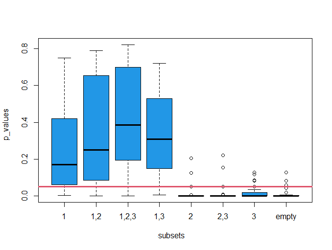
This result is not surprising. It is expected that the extremal dependence decreases with increasing distance. The effect of on the extremal dependence is shown in Figure 10. The fact that was not marked as a cause is not surprising either. We would need much stronger interventions and changes in time observations to detect anything. Additionally, it is unclear how time can cause extremal dependence (there may be several time-changing factors, but we do not know them explicitly). As for , it seems that the type of the site is not a direct cause of the extremal dependence.

6 Conclusion
This paper addresses the problem of causal discovery in the area of multivariate extremes. For a covariate-dependent extremal coefficient between two variables, we discover which of the covariates are not only significant but have a causal influence on the joint tail behavior. We introduced a LogMax-projection, which serves as a basis variable for inference about the extremal coefficient. A causal methodology from Peters et al. 2016 was adapted in our context to estimate the causal covariates. Algorithm (3.3) provides a consistent methodology. We used a very flexible GAM modelling for statistical inference.
We stress that the results rely on the absence of a hidden confounder, an assumption that can and should be debated in many situations. The methodology is robust against hidden covariates to some extent. However, if there is a hidden covariate, it must be invariant between environments. We discussed in simulations in Section 4 the case in which this assumption is violated.
We believe that this methodology can be very useful in many fields. More practical examples come from econometrics. We often see an extremal dependence between stocks. If one stock has a massive fall, other stocks seem to follow this fall too. Exploiting the causes of such behavior can be very useful and can broadly impact the field.
Possible future work can relate to the more general multivariate extensions of our methodology. We introduced LogMax-projection to work only with a univariate variable representing a complex multivariate tail dependence structure. However, it can be interesting to work directly with a tail dependence structure of multivariate random variables with dimensions more than and infer which covariates are significant and causal.
Conflict of interest
The authors declare that they have no known competing financial interests or personal relationships that could have appeared to influence the work reported in this paper.
Acknowledgements
The work was supported by the Swiss National Science Foundation.
References
- Beirlant et al. (2006) J. Beirlant, Y. Goegebeur, J. Segers, J.L. Teugels, D.D.Waal, and C. Ferro. Statistics of Extremes: Theory and Applications. Wiley Series in Probability and Statistics. Wiley, 2006.
- Bühlmann (2020) P. Bühlmann. Invariance, causality and robustness. Statistical Science, 35(3):404 – 426, 2020. doi: 10.1214/19-STS721.
- Carslaw and Ropkins (2022) D. C. Carslaw and K. Ropkins. Openair — an R package for air quality data analysis. Environmental Modelling and Software, 2022. ISSN 1364-8152. doi: 10.1016/j.envsoft.2011.09.008.
- Chang et al. (2015) R. Chang, J.R. Karr, and E.E. Schadt. Causal inference in biology networks with integrated belief propagation. Pac Symp Biocomput, pages 359–370, 2015. doi: 10.2307/1968974.
- Coles (2001) S. Coles. An Introduction to Statistical Modeling of Extreme Values. Springer Series in Statistics. Springer-Verlag, 2001. ISBN 1-85233-459-2.
- Coles and Tawn (1991) S.G. Coles and J. A. Tawn. Modelling extreme multivariate events. Journal of the Royal Statistical Society. Series B (Methodological), 1991. ISSN 00359246. URL http://www.jstor.org/stable/2345748.
- Dawid (2006) A. P. Dawid. Counterfactuals, hypotheticals and potential responses: a philosophical examination of statistical causality. Technical report, Department of Statistical Science,University College London, Research Report, 2006.
- Deuber et al. (2021) D. Deuber, J. Li, S. Engelke, and M. Maathuis. Estimation and inference of extremal quantile treatment effects for heavy-tailed distributions. preprint, 10 2021. doi: 10.48550/arXiv.2110.06627.
- Eberhardt and Scheines (2007) F. Eberhardt and R. Scheines. Interventions and causal inference. Philosophy of Science, 2007. URL http://www.jstor.org/stable/10.1086/525638.
- Engelke and Ivanovs (2021) S. Engelke and J. Ivanovs. Sparse structures for multivariate extremes. Annual Review of Statistics and Its Application, 8(1):241–270, 2021. doi: 10.1146/annurev-statistics-040620-041554.
- Engelke et al. (2015) S. Engelke, A. Malinowski, Z. Kabluchko, and M. Schlather. Estimation of Hüsler–Reiss distributions and Brown–Resnick processes. Journal of the Royal Statistical Society. Series B (Statistical Methodology), 2015. URL http://www.jstor.org/stable/24774733.
- Fisher and Tippett (1928) R.A. Fisher and L.H.C. Tippett. Limiting forms of the frequency distribution of the largest or smallest member of a sample. Mathematical Proceedings of the Cambridge Philosophical Society, 24(2):180–190, 1928. doi: 10.1017/S0305004100015681.
- Gnecco et al. (2020) N. Gnecco, N. Meinshausen, J. Peters, and S. Engelke. Causal discovery in heavy-tailed models. The Annals of Statistics, 49, 2020. doi: 10.1214/20-AOS2021.
- Gnedenko (1943) B. Gnedenko. Sur la distribution limite du terme maximum d’une serie aleatoire. Annals of Mathematics, 44(3):423–453, 1943. doi: 10.2307/1968974.
- Green and Silverman (1994) P. Green and B. Silverman. Nonparametric Regression and Generalized Linear Models: A Roughness Penalty Approach. Chapman and Hall/CRC, 1994. ISBN 9780412300400. URL https://www.routledge.com/Nonparametric-Regression-and-Generalized-Linear-Models-A-roughness-penalty/Green-Silverman/p/book/9780412300400.
- Haavelmo (1944) T. Haavelmo. The probability approach in econometrics. Econometrica, 1944. URL https://www.jstor.org/stable/pdf/1906935.pdf.
- Hamra et al. (2018) G.B. Hamra, F. Laden, A.J. Cohen, O. Raaschou-Nielsen, M.Brauer, and D. Loomis. Invariant causal prediction for nonlinear models. Journal of Causal Inference, 6(2), 2018. doi: 10.1515/jci-2017-0016.
- Heinze-Deml et al. (2018) C. Heinze-Deml, J. Peters, and N. Meinshausen. Invariant causal prediction for nonlinear models. Journal of Causal Inference, 6(2):20170016, 2018. doi: 10.1515/jci-2017-0016.
- Joe (1997) H. Joe. Multivariate Models and Multivariate Dependence Concepts, 1st Edition, volume 1. Chapman and Hall/CRC, 1 edition, 1997. URL https://doi.org/10.1201/9780367803896.
- Kiriliouk and Naveau (2020) A. Kiriliouk and P. Naveau. Climate extreme event attribution using multivariate peaks-over-thresholds modeling and counterfactual theory. The Annals of Applied Statistics, 2020. doi: 10.1214/20-AOAS1355.
- Mhalla et al. (2017) L. Mhalla, V. Chavez-Demoulin, and P. Naveau. Non-linear models for extremal dependence. Journal of Multivariate Analysis, 159:49–66, 2017. ISSN 0047-259X. doi: 10.1016/j.jmva.2017.04.006.
- Mhalla et al. (2019a) L. Mhalla, V. Chavez-Demoulin, and D.J. Dupuis. Causal mechanism of extreme river discharges in the upper Danube basin network. Journal of the Royal Statistical Society: Series C (Applied Statistics), 2019a. doi: 10.48550/ARXIV.1907.03555.
- Mhalla et al. (2019b) L. Mhalla, M. de Carvalho, and V. Chavez-Demoulin. Regression-type models for extremal dependence. Scandinavian Journal of Statistics, 46(4):1141–1167, 2019b. doi: 10.1111/sjos.12388.
- Mhalla et al. (2019c) L. Mhalla, T. Opitz, and V. Chavez-Demoulin. Exceedance-based nonlinear regression of tail dependence. Extremes, 22, 2019c.
- Pasche et al. (2021) O. C. Pasche, V. Chavez-Demoulin, and A.C. Davison. Causal modelling of heavy-tailed variables and confounders with application to river flow. Submitted, 2021. doi: 10.48550/ARXIV.2110.06686.
- Pauli and Coles (2001) F. Pauli and S. Coles. Penalized likelihood inference in extreme value analyses. Journal of Applied Statistics, 28(5):547–560, 2001. doi: 10.1080/02664760120047889.
- Pearl (2009) J. Pearl. Causality: Models, Reasoning and Inference. Cambridge University Press, 2009. ISBN 978-0521895606.
- Peters et al. (2014) J. Peters, J.M. Mooij, and B. Schölkopf. Causal discovery with continuous additive noise models. Journal of Machine Learning Research, 15:2009–2053, 2014.
- Peters et al. (2016) J. Peters, P. Bühlmann, and N. Meinshausen. Causal inference by using invariant prediction: identification and confidence intervals. Journal of the Royal Statistical Society: Series B (Statistical Methodology), 78(5):947–1012, 2016. URL https://doi.org/10.1111/rssb.12167.
- Peters et al. (2017) J. Peters, D. Janzing, and B. Schölkopf. Elements of Causal Inference: Foundations and Learning Algorithms. The MIT Press, 2017. ISBN 0262037319. URL https://library.oapen.org/bitstream/id/056a11be-ce3a-44b9-8987-a6c68fce8d9b/11283.pdf.
- Pfister and Peters (2022) N. Pfister and J. Peters. Identifiability of sparse causal effects using instrumental variables. Conference on Uncertainty in Artificial Intelligence, 2022. doi: 10.48550/ARXIV.2203.09380.
- Pickands (1975) J. Pickands. Statistical inference using extreme order statistics. The Annals of Statistics, 3(1):119 – 131, 1975. doi: 10.1214/aos/1176343003.
- Pickands (1981) J. Pickands. Multivariate extreme value distributions. Bull. Int. Statist. Inst. 49, pages 859–78, 1981.
- Razali and Yap (2011) N.M. Razali and B.W. Yap. Power comparisons of shapiro-wilk, kolmogorov-smirnov, lilliefors and anderson-darling tests. J. Stat. Model. Analytics, 2, 01 2011.
- Resnick (1987) S.I Resnick. Extreme Values, Regular Variation and Point Processes. Springer, NY, 1987. ISBN 978-0-387-75953-1. URL https://link.springer.com/book/10.1007/978-0-387-75953-1.
- Scholz and Stephens (1987) F.W. Scholz and M. A. Stephens. K-sample Anderson-Darling tests. Journal of the American Statistical Association, 82(399):918–924, 1987. doi: 10.2307/2288805.
- Schölkopf et al. (2012) B. Schölkopf, D. Janzing, J. Peters, E. Sgouritsa, K. Zhang, and J. Mooij. On causal and anticausal learning. In Proceedings of the 29th International Conference on Machine Learning (ICML), 2012. URL http://www.jstor.org/stable/10.1086/525638.
- Shi et al. (2014) P. Shi, P. Xie, M. Qin, F. Si, K. Dou, and K. Du. Cluster analysis for daily patterns of SO2 and NO2 measured by the DOAS system in Xiamen. Aerosol and Air Quality Research, 2014. doi: 10.4209/aaqr.2013.05.0160.
- Shimizu et al. (2006) S. Shimizu, P. Hoyer, A. Hyvärinen, and A. Kerminen. A linear non-gaussian acyclic model for causal discovery. Journal of Machine Learning Research, 7:2003–2030, 10 2006.
- Smith (1990) R.L. Smith. Extreme value theory. Handbook of Applicable Mathematics, (7):437–447, 1990.
- Spirtes et al. (2001) P. Spirtes, C. Glymour, and R. Scheines. Causation, Prediction, and Search, 2nd Edition, volume 1. The MIT Press, 1 edition, 2001. URL https://EconPapers.repec.org/RePEc:mtp:titles:0262194406.
- Tawn (1988) J.A. Tawn. Bivariate extreme value theory: Models and estimation. Biometrika, 75(3):397–415, 1988. doi: 10.2307/2336591.
- Tawn (1990) J.A. Tawn. Modelling multivariate extreme value distributions. Biometrika, 77(2):245–253, 1990. doi: 10.2307/2336802.
- Varian (2016) H. R. Varian. Causal inference in economics and marketing. Proceedings of the National Academy of Sciences, 113(27):7310–7315, 2016. doi: 10.1073/pnas.1510479113.
- Verma and Pearl (2013) T. S. Verma and J. Pearl. On the equivalence of causal models. CoRR, 2013. URL http://arxiv.org/abs/1304.1108.
- Wood et al. (2016) S. N. Wood, N. Pya, and B. Säfken. Smoothing parameter and model selection for general smooth models. Journal of the American Statistical Association, 111(516):1548–1563, 2016. doi: 10.1080/01621459.2016.1180986.
- Wood (2017) S.N. Wood. Generalized Additive Models: An Introduction with R. Chapman and Hall/CRC, 2 edition, 2017.
- Yoshida and Naito (2012) T. Yoshida and K. Naito. Asymptotics for penalized splines in generalized additive models. Journal of Nonparametric Statistics, 26, 08 2012. doi: 10.1080/10485252.2014.899360.
- Youngman (2020) B. Youngman. Generalised additive extreme value models. 2020. URL https://CRAN.R-project.org/package=evgam.