Pointer States in the Born-Markov approximation
Abstract
Explaining the emergence of classical properties of a quantum system through its interaction with the environment has been one of the promising ideas on how to understand the notorious quantum-to-classical transition. A pivotal role in this approach is played by, so called, pointer states which are quantum states least affected by the environment and are “carriers” of classical behavior. We develop here a general method on how to find pointer states. Working within the Born-Markov approximation, we combine methods of group theory and open quantum systems to derive explicit equations describing pointer states. They contain variances squared of certain operators, thus resembling the defining equations of coherent states, but are in general different from the latter. This shows that two notions of being “the closest to the classical” – one defined by the uncertainty relations and the other by the interaction with the environment – are in general different. As an example, we study arbitrary spin- systems interacting with bosonic or spin thermal environments and find explicitly pointer states for .
I Introduction
A comprehensive understanding of how the classical reality emerges from the underlying quantum theory is one of the biggest and most fascinating challenges of modern physics. In this context, decoherence program Zeh 1970; Joos et al. 2003; Zurek 2003; Breuer and Petruccione 2002; Schlosshauer 2007 has been highly successful in explaining the loss of quantum properties through the interaction with uncontrolled degrees of freedom (environment); see e.g. Chiorescu et al. 2003; Deléglise et al. 2008; Häffner et al. 2008; Hornberger et al. 2012; Moser et al. 2014; Tighineanu et al. 2018; Fein et al. 2019. The inevitable, in most realistic situations, interactions with the environment lead to delocalization and destruction of phase relations, making certain quantum superpositions unobservable. On the other hand, the same process distinguishes some preferred states Zurek 1981; Zurek 1982, which are least affected, and thus the system is most likely to be found in one of these states. In this sense, the perceived classicality can be explained through properties of certain robust quantum states Joos et al. 2003.
Determining the preferred states, known as pointer states, in the general case has been a difficult open task since their introduction in Zurek 1981. Several formal definitions were given with the most fruitful being the predictability sieve idea Zurek 1993, defining pointer states as states producing least entropy (for others see e.g. Diósi and Kiefer 2000). Various examples of pointer states have been found so far, with the the best known Zurek et al. 1993 in the Quantum Brownian Motion (QBM) model Feynman and Vernon 1963; Ullersma 1966; Joos et al. 2003; Schlosshauer 2007, where they happen to be the Glauber-Sudarshan coherent states Glauber 1963; Sudarshan 1963. Minimum uncertainty states were also proven to be universal pointer states for a general, linearly coupled free open evolution and that decoherence to them is generic Eisert 2004, which is an extension of an earlier result Diósi and Kiefer 2000, obtained in a simpler Markovian model. A general question when generalized coherent states Perelomov 1986 are the preferred states was analyzed in Boixo et al. 2007, using the Gorini-Kossakowski-Lindblad-Sudarshan (GKLS) Kossakowski 1972; Davies 1974; Gorini et al. 1976; Lindblad 1976 master equation and group-theoretical methods, showing that it is not generically the case unless specific conditions are met. Other results include Paraoanu and Scutaru 1998, where similar findings to Zurek et al. 1993 were derived in the GKLS formalism, Khodjasteh et al. 2011, where the problem of how to engineer the coupling to turn a given pure state into a pointer state was studied in a non-Markovian setup, and Donker et al. 2017 where pointer states for anti-ferromagnetic systems were numerically analyzed.
In this work we derive a general framework for finding pointer states in the Born-Markov approximation with a linear coupling. We do so under a broad assumption of an existence of some Lie group structure behind the dynamics, which covers, among others, the canonical models of decoherence Schlosshauer 2007. We analyze in detail the case of a compact, semi-simple group, but our method applies to other groups too as we show on the QBM example of Zurek et al. 1993. The resulting conditions take form of an optimization problem involving sum of variances of certain operators and are in general different from the ones defining coherent states for the group, confirming that open dynamics selects its own robust states, different from the static minimal uncertainty principle (cf. Boixo et al. 2007). As a concrete example, we apply our method to thermal spin models with arbitrary spin- central systems interacting with either bosonic or spin environments. For we explicitly find the pointer states.
The use of the Born-Markov rather than the GKLS approach can be criticized on the ground that it lacks complete-positivity, which has been a matter of an ongoing debate (see e.g. Winczewski et al. 2021; Tupkary et al. 2022 and the references therein), despite the immense predictive power of the former Schlosshauer 2007. We use the Born-Markov equation as it allows for a more direct connection with the underlying microscopic model by avoiding the secular approximation Breuer and Petruccione 2002 and the associated problems Tupkary et al. 2022. We stress that is not our aim to add to the debate but rather to exploit the potential of the Born-Markov equation in a search for pointer states.
The paper is organized is as follows: In Sec. II, we start with a general Born-Markov master equation and introduce the framework to incorporate a group structure on the free and the interacting Hamiltonians. Then based on this group structure, we derive our main result, namely, the conditions giving rise to the approximate pointer states. In Sec. III, we apply our framework to the example of QBM and discuss why the coherent states are the approximate pointer states in this particular case. In Sec. IV, we consider the example of spin- particles and show explicitly that the coherent states are not the approximate pointer states. Finally, we conclude in Sec. V with a discussion on ramifications of our results along with the future directions. In Appendix A, we provide detailed calculations for spin- example in various regions of temperature of the environment.
II Pointer states and group-theoretical methods in the Born-Markov approximation.
We consider an open system model, , where a system of interest , governed by the free Hamiltonian , is coupled to the environment via a bilinear interaction term . The most general coupling is a sum of such terms Schlosshauer 2007 and a generalization of our method to such couplings is straightforward. We will assume the weak-coupling limit and that the conditions of the Born-Markov approximation hold. Then system’s reduced density matrix satisfies the Born-Markov master equation Redfield 1957; Bloch 1957; Schlosshauer 2007:
| (1) |
where ,
| (2) |
and , are respectively the the noise and dissipation kernels defined via the environment correlation function:
| (3) |
. The environment state is arbitrary here as long as it is stationary , which is the standard assumption Joos et al. 2003; Breuer and Petruccione 2002; Schlosshauer 2007.
The predictability sieve looks for those states of the system, which generate the least entropy during the evolution (II). A convenient measure is the linear entropy (c.f. Diósi and Kiefer 2000; Zurek 2003):
| (4) |
connected to the loss of purity. We thus assume a pure initial state:
| (5) |
and ask how much of the purity is lost during the evolution Zurek et al. 1993. Let us now assume that there exists a Lie group of dimension , such that and are from the Lie algebra of and in particular can be represented using generators of :
| (6) | ||||
| (7) |
(we choose as one of the generators and leave arbitrary only for the sake of definiteness). This is somewhat similar to the approach of Boixo et al. 2007, however instead of imposing the secular approximation and studying the algebra generated by the GKLS jump operators and the associated generalized coherent states, we assume the existence of a dynamical group already at the microscopic level. Both and must be Hermitian for obvious physical reasons, which motivates the assumption that the Lie algebra in question is real and spanned by Hermitian operators, . Further assuming they can be represented in finite dimension, becomes a subgroup of sufficiently large unitary group and thus compact. In light of these identifications, the free evolution, given by Eq. (2), becomes the adjoint action of in its Lie algebra. In particular, we have
| (8) |
where . The indices are the Lie algebra indices of . Matrix is nothing but the exponent of the structure constants of , arranged into matrix (the matrix of the action) and is given by
| (9) |
where are defined via . In what follows we will omit the index for simplicity, writing . Substituting Eq. (8) into Eq. (II), we obtain
| (10) |
where we have introduced constants (assuming the correlation function (3) is regular enough for the integrals to exist):
| (11) |
We can now express the change of the entropy (4) as
| (12) |
To make the further analysis feasible, we may assume as a first approximation Zurek et al. 1993 that the state at the right hand side above is approximately pure and evolves according to the free evolution, i.e.,
| (13) |
Using Eq. (8) we obtain
| (14) | ||||
| (15) |
where
| (16) |
is the covariance matrix calculated in the initial state and is the average in the initial state.
To analyze Eqs. (14) and (15) further, we look closer at the structure of matrices . For compact group , there is a Killing-Cartan form, (see e.g. Kirillov Jr. 2008) on the Lie algebra of with a definite signature and which serves as a metric. Moreover, is preserved by the adjoint action (8). For simplicity, we will also assume that this metric is non-degenerate (so the group is semi-simple), but this is not crucial. We can then diagonalize the metric and assume so that the matrices of the adjoint action become orthogonal matrices. Since they are in the connected component of the unity by taking in Eq. (8), they are also special orthogonal, i.e. . Furthermore, from Eq. (8) we obviously have , i.e. the N-th row has just one element . From the orthogonality , the -th column has the same property and is of the form:
| (17) |
i.e. it is a rotation around the axis of as one could easily guess from Eq. (8). In most physical models the non-dynamical part of is usually neglected but we keep it here for completeness. The part can be further decomposed into a direct sum of rotations by a change of basis in the Lie algebra. For odd , i.e. even , one of the blocks will again be . Summarizing, we can write the following decomposition of the full matrix :
| (18) |
where (we prefer to use the full dimensional matrices extended by on the diagonal for the ease of the index notation later) and the last block . Additionally, for even the one before the last block is also trivial, i.e., we have
| (19) |
for odd and even , respectively. The form of the time dependence of rotations comes from the antisymmetry of the generator of the adjoint representation, Eq. (8), which in turn follows from the differential form of the invariance of the Cartan-Killing form:
| (20) |
making totaly anti-symmetric as by definition .
Summarizing, for each particular model, the l.h.s. of Eq. (14) is a finite linear combination of trigonometric functions and their squares, which, in principle, can be integrated (cf. Zurek et al. 1993). However, the instantaneous value of the entropy production may not be the most indicative quantity due to its time fluctuations. Here we choose its long-time average as more representative:
| (21) |
meaning we average the entropy production over times much longer than any other time scales. We apply the above time-averaging to Eq. (14) using Eq. (18). The first term gives
| (22) |
where are the matrices of embedded naturally into the whole space by adding rows and columns of zeros, i.e. when are outside of the -subspace. We have also used the fact that
| (23) |
for non-trivial blocks. Trivial blocks give simply . Here is the totally anti-symmetric Levi-Civita symbol in dimension two. Eq. (23) follows from a direct entry-by-entry averaging of , using the explicit form, Eq. (18), where only the quadratic terms with the same angular velocity, i.e., and , give non-zero contributions (We assume a generic situation with no special relations between eigenfrequencies for different ). Let us define rotated generators as
| (24) |
and the corresponding covariance matrix . We recall that by the construction of , cf. Eq. (17). We then have
| (25) |
where is the projection of on the -subspace and in the last step we used the symmetry of (inherited from ). Using this, we can write
| (26) |
where we introduced a rotated vector and decomposed the matrix by inserting decomposition, given by Eq. (18) into Eq. (11) and defined
| (27) |
The coefficients and are generalized normal and anomalous diffusion coefficients, corresponding to the eigenfrequency :
| (28) | ||||
| (29) |
We now substitute Eqs. (22), (25), and (26) into Eq. (14) to finally obtain
| (30) |
and for even there is an additional term . Here , is the norm squared of the projection of the vector on the -subspace. We used the fact that matrices and are supported in different subspaces for , and the explicit form, Eq. (27), to calculate the quadratic form. Further, in the last step we used the definition of , given by Eq. (16), but with the rotated generators (Eq. (24)). Moreover, , denote the two generators in the -subspace and are their variances in the initial state . Finally, we introduced , provided the integral exists (e.g. for Ohmic and super-Ohmic bosonic environments).
In the similar fashion we now analyze the term, Eq. (15), linear in . Let us first assume odd group dimension . It is then clear from Eqs. (17) and (18) that the only term that survives the time averaging is , the rest being zero, so that
| (31) |
where we have used the total antisymmetry of , cf. Eq. (20). Let us now decompose matrices and following the decomposition, Eq. (18). Substituting Eq. (18) into Eq. (11) we obtain
| (32) |
where
| (33) | ||||
| (34) |
are generalized frequency shift and the momentum damping coefficients, corresponding to the eigenfrequency (cf. Schlosshauer 2007). In the similar way, Eq. (18) implies via the differentiation of Eq. (9), the block-diagonal form of the matrix as
| (35) |
where the last block is zero due to Eq. (17). Recalling that ; using matrix/vector notation and the natural embeddings of and into the whole space, we obtain from Eq. (31) that
| (36) |
where we used the explicit forms of and and the fact that they are supported in different subspaces for . Thus, the linear term, Eq. (31), is equal to
| (37) |
For even dimension , the situation is more complicated. There is one more non-zero element in , corresponding to the element of the canonical form of : , cf. Eq. (19). It leads to an additional term in Eq. (31):
| (38) |
where is the ad operator of the transformed generator and is the matrix of transformed to the new basis so that . This is as much as can be said in a general case.
Summarizing, for an odd dimension , the asymptotic entropy production reads
| (39) | ||||
| (40) |
For even it reads
| (41) |
To simplify the above expressions further, let us consider a low-damping limit , which holds e.g. in high-temperature environments Schlosshauer 2007; Breuer and Petruccione 2002, and drop the non-dynamical term from Eq. (7) as it is usually the case. This gives:
| (42) |
where we introduced an environment-dependent metric
| (43) |
where for even the last non-zero block is equal to . There is a formal similarity between (42) and the definition of the generalized coherent states as the states that minimize the -invariant dispersion Perelomov 1986. However, the metric is in general different from the Killing-Cartan form , which here is . For example, in thermal models can non-trivially depend on the temperature via the diffusion coefficients . Thus the states minimizing Eq. (42) are in general different from the coherent states for unless or more generally Boixo et al. 2007.
Although we have assumed for definiteness’ sake a compact, semi-simple dynamical group , our method is not restricted to such groups only. We used the fact that , (9), is from a group with a known canonical form (18). It is clear that other groups with known canonical forms, e.g. symplectic, can be analyzed by the above method. It can also happen that a non-compact group leads to orthogonal as we show below.
III Quantum Brownian Motion case
It is interesting to revisit from the current perspective the seminal result of Zurek et al. 1993, which shows that for the quantum Brownian motion model the pointer states are the coherent states. The model is described by and . The group that can be associated with the dynamics is generated by the operators and is known as the oscillator group Streater 1967. The group is non-compact (it is a projective representation of ) but after the rescaling , , the matrix of the adjoint action (see Eq. (8)) generated by becomes orthogonal (with the Lie algebra basis and ). In particular,
| (44) |
The matrix is already in the canonical form, Eq. (19). We can thus use our procedure and obtain the high temperature entropy production equation (Eq. (42) with and the rest ’s zero):
| (45) |
Modulo an unimportant prefactor, the above equation is the same as obtained in Ref. Zurek et al. 1993 via a direct calculation. is given by Eq. (28) with . It now so happens that the r.h.s. of Eq. (45) corresponds to an invariant dispersion for a subgroup of –the Heisenberg-Weyl group generated by . The minimization of Eq. (45) leads to the coherent states of , which are the celebrated Glauber-Sudarshan coherent states Sudarshan 1963; Glauber 1963, and which are also coherent states for Perelomov 1986. This situation, however, is rather exceptional as e.g. it is well known that taking higher order than quadratic polynomials in , will not lead to any group structures, which in turn is connected to the problems of canonical quantization Groenewold 1946.
IV Spin- systems
As a further illustration, we consider a class of models where a central spin- interacts with a thermal environment. As our general method is quite insensitive to the type of the environment, as long as the auto-correlation function is sufficiently regular, it will not matter below if the environment is bosonic, with the total Hamiltonian:
| (46) |
or spin:
| (47) |
Above are the spin operators of the central system, are the Pauli matrices for the -th spin, are the annihilation and creation operators, respectively, of the environment, which is assumed to be thermal with the inverse temperature . Both spin-spin and spin-boson models have become of a significant importance recently due to their role in such fields as e.g. matter-wave interferometry Hornberger et al. 2012; Fein et al. 2019, quantum dots Urbaszek et al. 2013, nitrogen-vacancy centers Doherty et al. 2013, applied quantum information Bergou et al. 2021.
The models fall within our framework with , , . The adjoint matrix, Eq. (8), is then already in the canonical form and reads (after rescaling ):
| (48) |
From Eqs. (39) and (40), we immediately obtain the entropy production (with , the rest zero):
| (49) |
where are from (28), (34) and are given by the well-known expressions Schlosshauer 2007 with . Eq. (49), is the same, up to an irrelevant positive prefactor, for both models, which can be seen e.g. using the standard spin-oscillator mapping Schlosshauer 2007.
We simplify (49) here by considering the high temperature limit (cf. (42)):
| (50) |
The r.h.s. looks almost like the -invariant dispersion , which defines the spin coherent states Perelomov 1986, but without the last term. This absence of the -invariance, changes the minimization problem significantly (Eq. (50) is invariant only w.r.t. rotations ). To this end, let us assume that ’s describe a spin- system. It is then easy to calculate Eq. (49) for spin coherent states , where is a unit vector, , and . More precisely, we obtain:
| (51) |
with the minimum at leading to
| (52) |
In the special case of , the above equation implies . This is satisfied for spin- systems (e.g. a two-level atom), since then all pure states are coherent states by definition. However, this is not so already for spin-. As we show in Appendix A, the minimum for high temperature is achieved for the following family of states:
| (53) |
and the minimum value is given by
| (54) |
which is strictly lower than the minimum for spin coherent states. Although the overlap can be as high as for certain coherent states, the states are superpositions of two orthogonal spin coherent states, cf. (74), showing their “non-classicality” w.r.t. spin coherent states.
V Conclusions
Although the introduction of pointer states was arguably a serious conceptual step towards understanding of the quantum-to-classical transition and decoherence, there has been no systematic approach of studying them, apart from simplest situations. This work helps to fill this gap. We develop a general framework for finding pointer states within the Born-Markov approximation and with an additional assumption of a dynamical group structure. Satisfied in most important open systems models, the latter allows to use group-theoretical methods to find defining equations of pointer states in the weak-coupling limit. We study those equations in detail for spin- systems with either bosonic or spin environments.
We used mostly compact, semi-simple groups above but as we have mentioned the method is more universal and can be applied to other groups too. It is enough that the free evolution generates a group with some known canonical decomposition, like we showed on the QBM example and the oscillator group. The defining equations unfortunately present a difficult optimization problem even in the low-damping regime, as the spin models illustrate, and new mathematical tools will most probably be needed to tackle it. It would be also interesting to learn more about the physical characteristics of the states found here (we know they are not minimum uncertainty states) and understand if and how a general initial state of the system evolves towards their mixture (cf. Eisert 2004). And going one step further, if advanced quantum-to-classical transition mechanisms such as quantum Darwinism and Spectrum Broadcast Structures Zurek 2009; Korbicz et al. 2014; Le and Olaya-Castro 2019; Unden et al. 2019; Korbicz 2021 can be defined around them. We hope that our work will stimulate a further research into those and related topics and contribute to the debate on the dynamical emergence of classical properties in quantum systems.
Acknowledgements.
We would like to thank Lorenza Viola for valuable discussions and pointing us to some earlier works on pointer states. U.S. and J.K.K. acknowledge the support by Polish National Science Center (NCN) (Grant No. 2019/35/B/ST2/01896).References
- Zeh (1970) H. D. Zeh, On the interpretation of measurement in quantum theory, Found. Phys. 1, 69 (1970).
- Joos et al. (2003) E. Joos, H. D. Zeh, C. Kiefer, D. Giulini, J. Kupsch, and I.-O. Stamatescu, Decoherence and the Appearance of a Classical World in Quantum Theory (Springer Berlin, Heidelberg, 2003).
- Zurek (2003) W. H. Zurek, Decoherence, einselection, and the quantum origins of the classical, Rev. Mod. Phys. 75, 715 (2003).
- Breuer and Petruccione (2002) H.-P. Breuer and F. Petruccione, The Theory of Open Quantum Systems (Oxford University Press, 2002).
- Schlosshauer (2007) M. Schlosshauer, Decoherence and the Quantum-To-Classical Transition (Springer Berlin, Heidelberg, 2007).
- Chiorescu et al. (2003) I. Chiorescu, Y. Nakamura, C. J. P. M. Harmans, and J. E. Mooij, Coherent quantum dynamics of a superconducting flux qubit, Science 21, 1869 (2003).
- Deléglise et al. (2008) S. Deléglise, I. Dotsenko, C. Sayrin, J. Bernu, M. Brune, J.-M. Raimond, and S. Haroche, Reconstruction of non-classical cavity field states with snapshots of their decoherence., Nature 455, 510 (2008).
- Häffner et al. (2008) H. Häffner, C. Roos, and R. Blatt, Quantum computing with trapped ions, Physics Reports 469, 155 (2008).
- Hornberger et al. (2012) K. Hornberger, S. Gerlich, P. Haslinger, S. Nimmrichter, and M. Arndt, Colloquium: Quantum interference of clusters and molecules, Rev. Mod. Phys. 84, 157 (2012).
- Moser et al. (2014) J. Moser, A. Eichler, J. Güttinger, M. I. Dykman, and A. Bachtold, Nanotube mechanical resonators with quality factors of up to 5 million, Nature Nanotech 9, 1007–1011 (2014).
- Tighineanu et al. (2018) P. Tighineanu, C. L. Dreeßen, C. Flindt, P. Lodahl, and A. S. Sørensen, Phonon decoherence of quantum dots in photonic structures: Broadening of the zero-phonon line and the role of dimensionality, Phys. Rev. Lett. 120, 257401 (2018).
- Fein et al. (2019) Y. Y. Fein, P. Geyer, P. Zwick, F. Kiałka, S. Pedalino, M. Mayor, S. Gerlich, and M. Arndt, Quantum superposition of molecules beyond 25 kda, Nat. Phys. 15, 1242–1245 (2019).
- Zurek (1981) W. H. Zurek, Pointer basis of quantum apparatus: Into what mixture does the wave packet collapse?, Phys. Rev. D 24, 1516 (1981).
- Zurek (1982) W. H. Zurek, Environment-induced superselection rules, Phys. Rev. D 26, 1862 (1982).
- Zurek (1993) W. H. Zurek, Preferred States, Predictability, Classicality and the Environment-Induced Decoherence, Progress of Theoretical Physics 89, 281 (1993).
- Diósi and Kiefer (2000) L. Diósi and C. Kiefer, Robustness and diffusion of pointer states, Phys. Rev. Lett. 85, 3552 (2000).
- Zurek et al. (1993) W. H. Zurek, S. Habib, and J. P. Paz, Coherent states via decoherence, Phys. Rev. Lett. 70, 1187 (1993).
- Feynman and Vernon (1963) R. Feynman and F. L. Vernon, The theory of a general quantum system interacting with a linear dissipative system, Ann. Phys. 24, 118 (1963).
- Ullersma (1966) P. Ullersma, An exactly solvable model for brownian motion: I. derivation of the langevin equation, Physica 32, 27 (1966).
- Glauber (1963) R. J. Glauber, Coherent and incoherent states of the radiation field, Phys. Rev. 131, 2766 (1963).
- Sudarshan (1963) E. C. G. Sudarshan, Equivalence of semiclassical and quantum mechanical descriptions of statistical light beams, Phys. Rev. Lett. 10, 277 (1963).
- Eisert (2004) J. Eisert, Exact decoherence to pointer states in free open quantum systems is universal, Phys. Rev. Lett. 92, 210401 (2004).
- Perelomov (1986) A. Perelomov, Generalized Coherent States and Their Applications (Springer Berlin, Heidelberg, 1986).
- Boixo et al. (2007) S. Boixo, L. Viola, and G. Ortiz, Generalized coherent states as preferred states of open quantum systems, Europhysics Letters 79, 40003 (2007).
- Kossakowski (1972) A. Kossakowski, On quantum statistical mechanics of non-hamiltonian systems, Reports on Mathematical Physics 3, 247 (1972).
- Davies (1974) E. B. Davies, Markovian master equations, Commun. Math. Phys. 39, 91 (1974).
- Gorini et al. (1976) V. Gorini, A. Kossakowski, and E. C. G. Sudarshan, Completely positive dynamical semigroups of n‐level systems, J. Math. Phys. 17, 821 (1976).
- Lindblad (1976) G. Lindblad, On the generators of quantum dynamical semigroups, Commun. Math. Phys. 48, 119 (1976).
- Paraoanu and Scutaru (1998) G.-S. Paraoanu and H. Scutaru, Classical states via decoherence, Phys. Lett. A 238, 219 (1998).
- Khodjasteh et al. (2011) K. Khodjasteh, V. V. Dobrovitski, and L. Viola, Pointer states via engineered dissipation, Phys. Rev. A 84, 022336 (2011).
- Donker et al. (2017) H. C. Donker, H. De Raedt, and M. I. Katsnelson, Decoherence and pointer states in small antiferromagnets: A benchmark test, SciPost Phys. 2, 010 (2017).
- Winczewski et al. (2021) M. Winczewski, A. Mandarino, M. Horodecki, and R. Alicki, Bypassing the intermediate times dilemma for open quantum system (2021), arXiv:2106.05776 [quant-ph] .
- Tupkary et al. (2022) D. Tupkary, A. Dhar, M. Kulkarni, and A. Purkayastha, Fundamental limitations in lindblad descriptions of systems weakly coupled to baths, Phys. Rev. A 105, 032208 (2022).
- Redfield (1957) A. G. Redfield, On the theory of relaxation processes, IBM Journal of Research and Development 1, 19 (1957).
- Bloch (1957) F. Bloch, Generalized theory of relaxation, Phys. Rev. 105, 1206 (1957).
- Kirillov Jr. (2008) A. Kirillov Jr., An Introduction to Lie Groups and Lie Algebras, Cambridge Studies in Advanced Mathematics (Cambridge University Press, 2008).
- Streater (1967) R. F. Streater, The representations of the oscillator group, Commun. Math. Phys. 4, 217 (1967).
- Groenewold (1946) H. Groenewold, On the principles of elementary quantum mechanics, Physica 12, 405 (1946).
- Urbaszek et al. (2013) B. Urbaszek, X. Marie, T. Amand, O. Krebs, P. Voisin, P. Maletinsky, A. Högele, and A. Imamoglu, Nuclear spin physics in quantum dots: An optical investigation, Rev. Mod. Phys. 85, 79 (2013).
- Doherty et al. (2013) M. W. Doherty, N. B. Manson, P. Delaney, F. Jelezko, J. Wrachtrup, and L. C. Hollenberg, The nitrogen-vacancy colour centre in diamond, Physics Reports 528, 1 (2013), the nitrogen-vacancy colour centre in diamond.
- Bergou et al. (2021) J. A. Bergou, M. Hillery, and M. Saffman, Quantum Information Processing: Theory and Implementation (Springer International Publishing, Cham, 2021).
- Zurek (2009) W. H. Zurek, Quantum darwinism, Nat. Phys. 5, 181 (2009).
- Korbicz et al. (2014) J. K. Korbicz, P. Horodecki, and R. Horodecki, Objectivity in a noisy photonic environment through quantum state information broadcasting, Phys. Rev. Lett. 112, 120402 (2014).
- Le and Olaya-Castro (2019) T. P. Le and A. Olaya-Castro, Strong quantum darwinism and strong independence are equivalent to spectrum broadcast structure, Phys. Rev. Lett. 122, 010403 (2019).
- Unden et al. (2019) T. K. Unden, D. Louzon, M. Zwolak, W. H. Zurek, and F. Jelezko, Revealing the emergence of classicality using nitrogen-vacancy centers, Phys. Rev. Lett. 123, 140402 (2019).
- Korbicz (2021) J. K. Korbicz, Roads to objectivity: Quantum Darwinism, Spectrum Broadcast Structures, and Strong quantum Darwinism–a review, Quantum 5, 571 (2021).
Appendix A Spin- systems
Here we minimize analytically the entropy production for spin- systems. In this case can be written as
| (55) | ||||
| (56) |
Let the initial state be parametrized using the usual eigenstates of as follows:
| (57) |
We then have
| (58) | ||||
| (59) | ||||
| (60) |
Taking and , the Eq. (49) for spin- particles reads
| (61) |
We want to minimize above quantity as a function of , and . To this end define a Lagrangian function
| (62) |
where is a Lagrange multiplier. To obtain the minima, we set first order derivatives of wrt , and to zero. We have following:
| (63a) | ||||
| (63b) | ||||
| (63c) | ||||
| (63d) | ||||
| (63e) | ||||
| (63f) | ||||
For , we have following set of equations equivalent to above equations.
| (64a) | ||||
| (64b) | ||||
| (64c) | ||||
Taking , we have and , then the above equations become
| (65a) | ||||
| (65b) | ||||
| (65c) | ||||
In the case when , we can define , and . Combining above equations, we get the following cubic polynomial in terms of :
| (66) |
Let be a real solution to the above equation giving rise to the minima. Then the pure state achieving the minima in Eq. (A) is give by following parameters: are arbitrary real numbers and
| (67) |
The minimum value for the Eq. (A) is given by
| (68) |
A.1 High temperature regime
In this case, is a solution of the equation . Then the minimum of Eq. (A) is obtained for and the pure state achieving the minimum is given by
| (69) |
where . The minimum value of Eq. (A) is given by
| (70) |
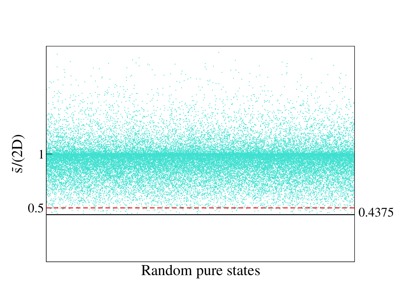
Figure 1 shows that indeed is the minimum value of . The random pure states on the plot are generated by first sampling two random complex numbers and one random real number using Mathematica functions and , respectively and then normalizing these three random numbers (cf. Eq. (57)). Further, for the state achieving the minima, we have
| (71) |
Their overlap with spin- coherent states is given by
| (72) |
where the maximum overlap is with the coherent state, given by
| (73) |
and reads . In the above, we have identified the coherent state with . Further, decomposing into spin-coherent states shows that it can be represented as a sum of two orthogonal coherent states:
| (74) |
A.2 Intemediate temperature regime,
In this case, is a solution of the equation . The minimum of Eq. (A) is obtained for . Then, the pure state achieving the minimum (that is the pointer state) is given by
| (75) |
where and
| (76) |
Then using Eq. (68), the minimum value of Eq. (A) is given by
| (77) |
Further, for the state achieving the minima, we have
A.2.1 Low temperature regime,
In this case, is a solution of the equation . The minimum of Eq. (A) is obtained for . Then, the pure state achieving the minimum (that is the pointer state) is given by
| (78) |
where or simply . The minimum value of Eq. (A) is given by
| (79) |
Further, for the state achieving the minima, we have
| (80) |
Figure 2 shows that the time averaged mixedness decreases as we decrease temperature.