Comparing the Locations of Supernovae to CO (2-1) Emission in their Host Galaxies
Abstract
We measure the molecular gas environment near recent ( yr old) supernovae (SNe) using or pc resolution CO (2-1) maps from the PHANGS-ALMA survey of nearby star-forming galaxies. This is arguably the first such study to approach the scales of individual massive molecular clouds ( M⊙). Using the Open Supernova Catalog (OSC), we identify 63 SNe within the PHANGS–ALMA footprint. We detect CO (2-1) emission near of the sample at 150 pc resolution, compared to of map pixels with CO (2-1) emission, and up to of the SNe at 1 kpc resolution compared to of map pixels with CO (2-1) emission. We expect the of SNe within the same 150 pc beam as a GMC will likely interact with these clouds in the future, consistent with the observation of widespread SN-molecular gas interaction in the Milky Way, while the other of SNe without strong CO (2-1) detections will deposit their energy in the diffuse interstellar medium (ISM), perhaps helping drive large-scale turbulence or galactic outflows. Broken down by type, we detect CO (2-1) emission at the sites of of our 9 stripped-envelope SNe (SESNe), of our 34 Type II SNe, and of our 13 Type Ia SNe, indicating that SESNe are most closely associated with the brightest CO (2-1) emitting regions in our sample. Our results confirm that SN explosions are not restricted to only the densest gas, and instead exert feedback across a wide range of molecular gas densities.
Keywords:
interstellar medium: star-formation – supernova: locations – galaxies: nearbyI Introduction
I.1 Overview
Feedback from supernovae (SNe) is among the most influential processes in galaxy evolution. SNe launch galactic winds (Chevalier & Clegg 1985; Veilleux et al. 2020, e.g.,), heat the interstellar medium (McKee & Ostriker 1977, ISM, e.g.,), regulate star formation (Kim & Ostriker 2015, e.g.,), and help set the balance between the gravitational and pressure forces within the disks of galaxies (Thompson et al. 2005; Ostriker & Shetty 2011; Sun et al. 2020, e.g.,). However, the exact effects of SNe on galaxies and giant molecular clouds (GMCs) depend on the locations where the SNe occur. SNe that occur in environments full of low-density gas cool slowly and hence are efficient at heating and ejecting material out of the galaxy, resulting in hot, diffuse gas outflows (Martizzi et al. 2016; Andersson et al. 2020; Lopez et al. 2020, e.g.). Conversely, SNe that occur in or near dense clouds can destroy GMCs and shut down star formation in these areas but cool more rapidly and hence are less effective at driving outflows (Walch et al. 2015; Keller & Kruijssen 2020; Lu et al. 2020). As a result, the impact of SNe on the ISM and their parent galaxies depends on the relative spatial configuration of the SNe, the gas, and the density distribution of that gas. However this relative configuration is not immediately obvious from first principles. Both thermonuclear (or Type Ia) SNe and core-collapse SNe (CCSNe) explode with delay times – i.e., the time since the formation of the stellar population – that can be long relative to the timescales over which the ISM evolves (see §I.1). Further complicating this picture is the finding that stars often form in clusters (Kruijssen 2012; Krumholz et al. 2019; Adamo et al. 2020) and theoretical models show that the clustering of SNe and feedback leads to more effective driving of outflows (Keller et al. 2022; Orr et al. 2022).
Despite the importance of this topic, we do not yet have a clear observational picture of where SNe explode relative to the gas in their host galaxies, partly because sensitive, high-resolution observation of cold, star-forming interstellar gas in distant galaxies was not possible until the advent of the Atacama Large Millimeter/Submillimeter Array (ALMA). Previous studies of SN environments have carried out detailed analyses focused on the stellar populations at the sites of SNe using ground-based optical telescopes (Anderson & James 2008; Anderson & James 2009; Anderson et al. 2012). In the more spatially-resolved environment of the Milky Way and Local Group galaxies, studies have focused on the interactions of supernova remnants (SNRs) and gas clouds (Jiang et al. 2010, e.g.,). There have also been studies of the properties and distributions of Hii regions and clouds, which suggest that pre-SN feedback mechanisms, such as stellar winds and ionizing radiation, can exert a strong influence (Lopez et al. 2011; Lopez et al. 2014; Kruijssen et al. 2019; Chevance et al. 2020; Barnes et al. 2021; McLeod et al. 2021; Olivier et al. 2021; Chevance et al. 2022, e.g.,). In the Milky Way, individual, young, massive star clusters show evidence of substantial feedback but no SN explosions (Zeidler et al. 2016; Beasor et al. 2021, e.g.,).
These studies only provide indirect or incomplete information on the gas in the environments where stars actually explode, or in the case of SNRs, measurements that occur after the SNe have processed the ISM (Sarbadhicary et al. 2017, e.g.,). A more direct, complementary measurement would be to measure the gas content at the sites of very recent SN explosions, taking advantage of high-resolution spectral-line observations enabled by ALMA. However, there has been only a small amount of such work and most of that has used low-resolution (kpc scale) gas data.
For example, in one of the only direct measurements of gas at the sites of SNe to date, Galbany et al. 2017 measured CO (2-1) emission from the sites of 26 SNe in the EDGE-CALIFA survey (Bolatto et al. 2017). While pioneering, this work was limited to a median resolution of kpc. This is far larger than the spatial scales on which SN feedback occurs ( pc) and is not sufficient to localize the relative positions of individual SNe and GMCs.
A key next step is to measure the molecular gas present in the local environments of SN explosion sites on GMC scales ( pc). Such measurements will more directly access the mean densities where SNe explode and will help inform SN placement in galaxy evolution simulations. By sorting these measurements by SN type, one can study how the explosion landscape depends on the lifetime of the SN progenitor and how each class of SNe impacts its galactic environment. Given observations with high enough resolution, one might even directly measure the fraction of SNe that may help to disperse GMCs. Such measurements will be critical to assess the quantitative role of SNe in the evolution of the ISM, the launching of galactic winds, and of setting star formation rates (SFRs) and efficiencies. The obstacle has been assembling a large enough sample of recent SNe with accompanying high-resolution gas observations.
In this paper, we measure the molecular gas content at high (150 pc) spatial resolution at the sites of 63 recent ( yr) SN explosions. To do this, we take advantage of the PHANGS--ALMA11 1 “Physics at High Angular resolution in Nearby GalaxieS with ALMA”. For more information, see www.phangs.org. CO (2-1) survey (Leroy et al. 2021b), which mapped the molecular gas content of 90 of the nearest galaxies at pc resolution.
I.2 Background
This work focuses on characterizing the local environments of recent SNe. Previous SN environment studies (James & Anderson 2006; Anderson & James 2008; Anderson & James 2009; Kelly et al. 2008; Habergham et al. 2010; Habergham et al. 2012; Galbany et al. 2012; Galbany et al. 2014; Galbany et al. 2017; Anderson et al. 2012; Kangas et al. 2013; Anderson et al. 2015a; Anderson et al. 2015b; Audcent-Ross et al. 2020; Cronin et al. 2021) have employed pixel statistics and radial distribution comparisons to cross-correlate different types of SNe with tracers of star formation and stellar populations and assess the impact and likely progenitors of SNe. See Anderson et al. 2015b for a more thorough review.
These studies have helped inform our emerging picture of SNe. Core-collapse supernovae (CCSNe, such as Type Ib/Ic and Type II) are triggered by the collapse of the inert Fe-core of massive stars, occurring on timescales that decrease as the progenitor mass increases, down to a minimum of 4 Myr for stars of 60 and above (see reviews by Smartt 2009; Müller 2016). Stripped-envelope SNe (SESNe), such as SNe IIb, Ib, and Ic, are CCSNe that have lost some or all of their hydrogen (SNe IIb & SNe Ib) and helium (SNe Ic) envelopes prior to explosion. SESNe have high-mass progenitors, with observations that support an increasing mass range from SNe IIb-Ib-Ic, with SNe Ic coming from the youngest population of progenitors (Kelly et al. 2008; Anderson & James 2009). Because they arise from these very young stars, SNe Ic have the strongest association with other signatures of recent star formation out of all of the SNe types, and SESNe have stronger associations with star-forming regions than SNe II (Anderson et al. 2012; Galbany et al. 2017).
SNe Ia are the thermonuclear explosions of white dwarf stars in binary systems (see review by Maoz et al. 2014). These explosions have a comparatively long delay time relative to CCSNe, often described as a power law distribution with approximately equal SNe per logarithmic time interval (Maoz et al. 2014; Maoz & Graur 2017). This implies that many SNe Ia will explode long after their natal cloud and stellar population have dissipated. Due to the longer delay time of SNe Ia, their explosions should track the overall distribution of stellar mass better than recent star formation, reflecting that they arise from stars with a broad range of ages (Anderson et al. 2015a, e.g., see). This may also lead us to expect a relatively weak correlation between the location of SNe Ia and the gas clouds that host star formation.
The massive stars that produce CCSNe are formed in GMCs. These stars have lifetimes ranging from 3--50 Myr22 2 Calculations from Leitherer et al. 2014 find that the approximate time from zero-age main sequence to the first SN explosion is Myr. The shortest lifetimes of the most massive stars converge to 2.5 Myr (Choi et al. 2017), but stars more massive than 30 have decreased explodability (Sukhbold et al. 2016). It seems likely that the first SN explosion is Myr after the birth of a fully sampled initial mass function (IMF), but in some regions this may be longer due to incomplete sampling of the IMF (Chevance et al. 2022)., with some rarer instances extending the tail of the delay time distribution past 100 Myr33 3 These include electron-capture supernovae arising from super-AGB stars (Prieto et al. 2008; Thompson et al. 2009) and the merger of binaries, which produce a tail of explosions in binary population synthesis out to 100-200 Myr (Zapartas et al. 2017). Because of the short lifespans of the higher-mass range of CCSNe progenitors, one would expect that a fraction of CCSNe should be closely associated with molecular gas. However there are two known complications that we must consider: pre-SN feedback on the molecular gas and the non-trivial fraction of these massive stars that have moved away from their birth site.
Previous observational work has shown that massive stars exert strong feedback on their immediate environment in the form of winds and radiation even before they explode. This pre-SN feedback has been characterized by comparing individual pressures within Hii regions (Lopez et al. 2011; Pellegrini et al. 2011; Lopez et al. 2014; McLeod et al. 2020; Barnes et al. 2021; Olivier et al. 2021, e.g.) and by contrasting the distributions and fluxes of H to CO (2-1) emission within star-forming regions of galaxies (Schruba et al. 2010; Kruijssen et al. 2019; Schinnerer et al. 2019; Chevance et al. 2020; Chevance et al. 2022; Kim et al. 2022; Pan et al. 2022). As discussed by Kruijssen et al. 2019 and Chevance et al. 2020; Chevance et al. 2022, the existence of widespread H emission without associated CO (2-1) implies rapid clearing of molecular gas by stellar feedback. As a consequence of this, GMCs have been observed to have lifespans on the order of 5-30 Myr (e.g., see Kawamura et al. 2009; Fukui & Kawamura 2010; Meidt et al. 2015; Corbelli et al. 2017; Grasha et al. 2018; Grasha et al. 2019; Kruijssen et al. 2019; Chevance et al. 2020; Kim et al. 2021; Kim et al. 2022, J. Turner et al. ApJ in review).
Previous theoretical work (Krumholz & Matzner 2009; Murray et al. 2010; Stinson et al. 2013; Geen et al. 2016; Gatto et al. 2017; Rahner et al. 2019; Lucas et al. 2020; Keller et al. 2022, e.g.) has also emphasized the crucial role played by pre-SN feedback processes in regulating the star formation efficiency of GMCs, and the impact that the SN environment has on the effectiveness of SN feedback (Walch et al. 2015; Iffrig & Hennebelle 2015; Ohlin et al. 2019; Andersson et al. 2020, see e.g.). Modern simulations (Dobbs & Pringle 2013; Kim et al. 2018; Benincasa et al. 2020, e.g.) that model stellar feedback find the majority of these clouds live only 5–7 Myr with only a small percentage surviving to 20 Myr.
Even without clearing the parent cloud by pre-SN feedback, it may be possible for massive stars to separate from their birth site before they explode as SNe. Only the most massive O stars have lifetimes as short as 2.5 Myr, but most CCSNe have B star progenitors which have delay times on the order of 10-40 Myr. Assuming the relative velocity between progenitors and their natal molecular clouds (MCs) is on the order of the velocity dispersion of individual stellar associations (e.g. 10 km/s 10 pc/Myr), we would expect that they would move 100-400 pc before exploding in that delay time. Most of these stars will have traveled far enough away from their natal cloud to explode in diffuse regions of the galaxy. Aadland et al. 2018 found that in Local Group galaxies, red supergiants (progenitors of Type II SNe) are offset by nearly 200-600 pc from the nearest blue, main-sequence star, and twice as isolated as higher-mass stars (e.g., Wolf-Rayets). Previous observational work has shown that 20-30% of OB stars appear in the field (Oey et al. 2004; Gies 1987) in regions that are not associated with GMCs. Up to 46% of O stars and 4% of B stars have been observed to have “runaway” velocities of at least 30 , leading them to be found at large distances from their galactic birth site (Stone 1991; Russeil et al. 2017). Therefore, in the scenario where GMCs are not destroyed by pre-SN feedback, there can still be a significant fraction of CCSNe that are not coincident with molecular gas because the stars have moved away.
Because of the complexities discussed above, a priori predictions of where SNe occur relative to the gas in galaxies are complicated. The uncertainty and new information about pre-SN feedback, motions of stars, progenitors, etc., adds layers of complexity to this problem. In this paper, we make a series of measurements aimed at improving our knowledge of where SNe explode via direct observations. We measure the surface density and mass of molecular gas at the sites of recent explosions, measure the distance to the nearest detectable concentration of molecular gas, and examine how these results depend on physical resolution.
In §II, we identify all SNe that have recently occurred in the footprint of the PHANGS–ALMA CO (2-1) maps. In §III, we present our results as follows: In §III.1, we measure the signal-to-noise of the CO (2-1) emission at the location of each SN at multiple resolutions from 60 pc-1 kpc. This yields a basic measurement of how often molecular gas appears associated with the SN explosion sites and how this changes as a function of scale. In §III.2, we compare the distribution of CO (2-1) emission intensities at the location of the SN sample to the full intensity distribution in the galaxies at our most complete resolution of 150 pc. We estimate the corresponding mass and surface density of molecular gas. We then investigate how these distributions change as a function of SN type. In §III.3, we compare the molecular gas surface density distributions for the SN explosion sites and for the full set of pixels in the CO (2-1) maps at resolutions from 60-150 pc. In §III.4 we look at cut-outs of each individual SN site at the highest resolution CO (2-1) map available to see if the fraction of SN environments coincident with molecular gas changes at smaller scales and to classify the potential feedback from each SN. In §III.5, we measure the distribution of distances from our SN sample to the nearest location with well-detected molecular gas and the distribution of molecular gas surface densities. We then compare these distributions to several model populations of SNe. Finally, in §IV, we discuss the significance of our results.
II Methods
To explore the relationship between SNe and their natal GMCs, we first aim to identify all recent SNe that have exploded in the PHANGS–ALMA footprint and measure the molecular gas content of the ISM near these explosions. To do this, we select SNe from the Open Supernova Catalog (OSC; Guillochon et al. 2017), accessed on 2021 May 25, which includes almost all known recent SNe by blending a heterogeneous collection of all available previous surveys.
Our initial sample consists of all of the OSC objects located within the PHANGS–ALMA CO (2-1) mapping footprint that include a discovery date. By requiring a discovery date, we limit the sample mostly to SNe that have occurred in the last years. The earliest SN in our sample was recorded in 1901, and the median discovery date was 2003. PHANGS–ALMA has a resolution of pc, and even with high shock velocities of km s-1, a SN will only impact pc in 100 years. By contrast, if we included SNRs, which can remain detectable for years (Sarbadhicary et al. 2017), we would expect to see frequent signatures of interaction between SNRs and clouds and note that some SNe might have already cleared their parent cloud. We focus on recent SNe because we want to study the environments before the explosions have had time to strongly influence their surroundings.
In Table , we list the OSC object name, reported type, parent galaxy, and coordinates. We also include the reference paper for the astrometry and SN type or the discovery announcement if a reference paper with typing is not available44 4 Note that for two of the OSC objects (PTSS-19clju and PSN+204.332083-29.896833) we are unable to find a reference, and those are not included in our final, working sample.. Finally, we note whether the object is included in our working SN sample.
We caution that the OSC is heterogeneous. It includes all discovered SNe but without assurances of completeness. Many of the SNe in the OSC are discovered via targeted galaxy searches, which introduces a bias towards more massive host galaxies. Because more massive host galaxies have higher star formation rates and higher molecular gas surface densities, this bias could increase the frequency in which we find SNe coincident with molecular gas. SN searches, especially early searches, also show some bias against finding SNe near the bright center of galaxies (Holoien et al. 2019, e.g., see), and we would expect them to also be biased against finding the most heavily embedded SNe due to extinction. Because of this, we might miss SN populations located in high-extinction regions, which would decrease the fraction of SNe found coincident with molecular gas and limit the association that we measure between SNe and the highest density environments.
We consider galaxies targeted by the PHANGS–ALMA survey (Leroy et al. 2021b) which includes a representative sample of 90 relatively massive, actively star-forming, local ( Mpc) galaxies. This survey used the Atacama Large Millimeter/submillimeter Array (ALMA) to map CO (2-1) emission on pc scales. CO (2-1) emission is a standard tracer of the distribution of molecular gas in galaxies (Bolatto et al. 2013, for a review see), tracing the cold, dense, star-forming phase of the ISM. The PHANGS–ALMA survey covers of the CO (2-1) emission and active star formation, as traced by WISE emission, in each galaxy. We checked each SN entry in the OSC to see if the host was a member of PHANGS–ALMA or if the coordinates lay within the astrometric footprint of the PHANGS–ALMA CO (2-1) integrated intensity map. We verified the host galaxy assignment and SN type classification via discovery/follow-up papers for each individual SN (see Table ). We then verified by eye that the SNe indeed lie within the CO (2-1) maps. The PHANGS–ALMA footprint does not cover the outer disk regions of the galaxies surveyed. Because of this, we will miss any SNe that occur in these outer regions. This introduces a bias where fewer SNe will be associated with these lower-density environments. The PHANGS–ALMA survey also cannot “see” all of the molecular gas in the regions that are surveyed. The completeness will cause a underreporting of SN-CO interactions occurring in low-density environments.
We find 78 OSC objects in 33 galaxies within the PHANGS–ALMA footprint (see Table ). Of these, we discard a luminous red nova (LRN) reported in the catalogue (AT2020nqq), 7 SN candidates (AT2018eoq, AT2019pck, AT2019npi, AT2019npd, AT2020cwh, AT2020hol, AT2020juh), the second entry of a SN reported by two groups under two different names (SN2019ehk – classified as SN type Ib & PTSS-19clju – listed as unclassified), and two Type II SNe that occurred on the edge of the mapped region of NGC0628 (SN2003gd) and NGC4945 (SN2005af) where the CO (2-1) data appeared noisier and the image quality poorer. (SN1992eu also falls along the edge of NGC1097’s map, but we keep it in the sample because the map quality appeared fine at its position.) We also discard PSN204.33208329.896833 in NGC 5236, which has minimal reported data and is outside of the mapped region of the galaxy. Finally, we remove three SNe (SN1997bs, SN2019krl, SN2019qyl) from our sample because of uncertainty in their type classification and the liklihood that they are instead non-terminal explosions (Adams & Kochanek 2015; Andrews et al. 2021; Jencson et al. 2021; Ransome et al. 2021). This brings our sample size to 63 SNe within 31 galaxies.
We are interested in the coincidence of SNe and molecular gas; this measurement will be limited by the resolution of the ALMA data and the positional accuracy of the SN location determination. The ALMA astrometry is phase-referenced to quasars with well-determined locations, and we do not expect the absolute astrometric calibration of the ALMA data to represent a limiting factor at the scales we work at (see ALMA Technical Handbook). Instead the resolution of the ALMA data will usually represent the limiting factor, though for the older half of our sample the location of the SNe may also contribute uncertainty. The OSC does not include positional uncertainty estimates, so to gauge the level of uncertainty we examined the original reference papers (listed in Table ) to estimate the typical positional uncertainty. Many papers do not report a positional uncertainty (Martin et al. 2005; Marples & Bock 2016; Kendurkar 2018; Tonry et al. 2020, e.g.,) though reporting uncertainties has become more common for SN that have occurred in the last years. When positional uncertainties are reported, they tend to range from 0.1 to 1” (Evans & McNaught 2003; Monard 2008a; Pignata et al. 2009, e.g., see). Based on this, we assume that for modern SN searches like ASAS-SN (Shappee et al. 2014; Kochanek et al. 2017), represents a typical uncertainty on the position of a relatively recent SN without extensive follow up observations, meaning that we expect the SNe to be reasonably well determined relative to the ALMA resolution. However for early SNe, like SN1923A or 1935C in our sample, positional uncertainties could be as high as . We consider that for the (27/63) of our sample that has occurred within the last years, the positional uncertainty is better than the angular resolution of PHANGS–ALMA CO maps, while for the remaining (36/63), the uncertainty in the astrometry is dominated by the uncertainty in the reported SN location. We proceed, noting that this situation could be improved by more ALMA observations focused on modern SNe with well-determined locations or by simply waiting for more SNe to explode in the PHANGS targets.
For each SN in the PHANGS–ALMA footprint, we measure the line-integrated CO (2-1) intensity, expressed in the units of K km s-1, at the pixel location of the SN in the PHANGS–ALMA “broad” moment 0 map and its associated statistical uncertainty. The “broad” mask is the PHANGS high completeness data product, expected to include all emission but with somewhat higher noise. Leroy et al. 2021b describe the masking scheme and the procedure used to generate uncertainty maps. Briefly, the mask includes any regions of the data cube detected at either coarse or high resolution. The associated uncertainty map is calculated based on a three-dimensional noise model derived from the empty regions of the data cube and then converted into the map following standard error propagation. The PHANGS--ALMA survey55 5 PHANGS–ALMA survey data is available at https://almascience.eso.org/alma-data/lp/PHANGS. produced broad moment 0 maps at fixed physical resolutions of 60, 90, 120, 150, 500, 750, and 1000 pc, as allowed by the angular resolution of the data and the distance to the targets. We report our CO (2-1) intensity measurements at the pixel location of the SN sites and their statistical uncertainty in Table Comparing the Locations of Supernovae to CO (2-1) Emission in their Host Galaxies at resolutions of 60, 90, 120, and 150 pc.
This can be translated to a mass surface density of molecular gas, expressed in the units of , via:
| (1) |
where is the integrated CO (2-1) line intensity expressed in the units of K km s-1, is the CO (2-1) to H2 conversion factor, which represents the ratio of the gas mass-to-CO (2-1) luminosity and has units of [ (K km , and i is the inclination of the host galaxy (see Sun et al. 2022, for a discussion of the need to apply an inclination correction even at these scales).
We adopt the metallicity-dependent values calculated in Sun et al. 2020 which uses local metallicities predicted from scaling relations (Sánchez et al. 2014; Sánchez et al. 2019) and converts them to via a simple power-law scaling (similar to Accurso et al. 2017). We convert from to with a CO (2-1)-to-CO (1-0) line ratio value, (den Brok et al. 2021; Leroy et al. 2021a). Because the lower resolution of the data led it to be omitted from the Sun et al. 2020 calculations, we lack an estimate for NGC1068; instead we use the standard value of 6.7 (K km prescribed in Bolatto et al. 2013. We calculate the total molecular mass within each resolution element, , via:
| (2) |
where is the molecular gas surface density expressed in units of , and is the FWHM beam size of the CO (2-1) map in units of parsecs.
We calculate a representative and molecular gas mass measurement for our sample to highlight the general sensitivity of the CO (2-1) maps. We do this by measuring each value from all of the CO (2-1) maps in our sample – accounting for each galaxy’s inclination – and then taking the median value. We do the same for our molecular gas mass value. Note that because we account for the galaxies’ inclinations when calculating , there is not a single one-to-one mapping between molecular gas mass and that applies across the entire sample. We measure a median of and a median molecular gas mass of at 150 pc resolution.
In §III.5 we generate model SN populations from the probability distributions of the gas and stellar populations of our galaxies. The density of stellar populations is pulled from 3.6 m maps from the Infrared Array Camera (IRAC) on Spitzer. The provenance of the IRAC maps is described in Querejeta et al. 2021; most come from S4G (Sheth et al. 2010). We used 3.4 m Wide-field Infrared Survey Explorer (WISE) maps (Leroy et al. 2019) when IRAC maps are unavailable (for galaxies: Circinus, NGC2997, NGC4945, NGC5128, NGC5530, and NGC6744).
III Results
Our final cleaned sample consists of 63 SNe within 31 galaxies, each marked with a checkmark in Table . Overall, our SNe host galaxies have higher mass and higher SFR than the typical PHANGS–ALMA target. The median galaxy with a SNe has and while the median PHANGS–ALMA galaxy has and . This appears consistent with the idea that the SNe rate will broadly trace the SFR or stellar mass of a galaxy, making the more massive, more actively star-forming targets more likely to host a SNe, but the incompleteness of the OSC prevents any formal rate calculation.
Table III shows the distribution of the different SNe types in our sample. We divide our SNe into the following SN type classifications: SNe Ia, SNe II, Stripped-Envelope Supernovae (SESNe), and unclassified SNe. The SESNe consist of SNe Types Ib, Ic, and IIb. The unclassified SNe are either reported in the OSC as “unclassified” or as Type I SNe. The latter classification of Type I means that there were no hydrogen features in the spectrum used to classify the SN, but this does not provide enough information to distinguish between a CCSN or SN Type Ia.
| Type | Number | % of Sample | % of Classified |
|---|---|---|---|
| SNe II | 34 | 54 | 61 |
| SNe Ia | 13 | 21 | 23 |
| SESNe (IIb/Ib/Ic) | 9 | 14 | 16 |
| Unclassified | 7 | 11 | – |
| All types | 63 | 100 | – |

.


Figure 1c shows the PHANGS–ALMA CO (2-1) emission maps of the galaxies that host the SNe in our sample. The legends report the designation of the SN and its type classification.
III.1 Detection of CO (2-1) at the location of recent supernovae
First, we measure how frequently CO (2-1) emission is detected coincident with the sites of recent SNe. To do this, we use the signal-to-noise ratio measured from the PHANGS–ALMA intensity maps described in §II. For this exercise, we define signal-to-noise as a detection of molecular gas. We repeat this exercise for multiple resolutions, from 60 pc to 1 kpc. We show the results of these measurements in Figure 2 and Table III.1.
We detect CO (2-1) emission at (59/63) of the SN locations at 1 kpc resolution. Out of the 63 SNe, four66 6 SN1988M in NGC4496A, SN1999eu in NGC1097, SN2005df in NGC1559, SN2012A in NGC3239 do not have CO (2-1) detections coincident with their locations on kpc scales. These four are near map edges, and thus their non-detections are ambiguous. Finding CO (2-1) emission at the location of almost every SN at 1 kpc resolution may not be surprising. The PHANGS–ALMA survey targets star-forming galaxies, the survey area was chosen to match the extent of infrared (IR) emission in the galaxy, and the PHANGS–ALMA maps have very good surface brightness sensitivity at kpc resolution (Leroy et al. 2021b, see). Accordingly, in Sun et al. 2022, of the 1.5 kpc-size regions covering the complete PHANGS–ALMA survey show some detectable CO (2-1) emission. Thus, at kpc resolution, our observations mostly show that we are studying the the gas-rich, star-forming parts of star forming galaxies.
As the resolution improves, the fraction of CO (2-1) detections at the locations of recent SNe decreases. This reflects the combination of two effects:
- 1.
At coarser resolutions, a beam will be more likely to cover both a SN and nearby gas clouds that may not be directly coincident or physically associated with the SN. Scales of 150-500 pc correspond roughly to the range of distances between individual molecular gas peaks in PHANGS–ALMA (Chevance et al. 2020; Kim et al. 2022, J. Machado et al. in prep), so that at these resolutions it becomes increasingly likely to find a CO (2-1) peak within a randomly placed beam.
- 2.
The RMS noise of the CO (2-1) maps increases as the resolution becomes sharper. This means that while faint, diffuse CO (2-1) emission could be detected on 1 kpc scales, only gas with higher surface or column densities will be detected on 50–150 pc scales.
In massive (), CO-bright galaxies, the first effect is likely dominant, because the PHANGS--ALMA CO (2-1) maps have high completeness77 7 Completeness is the ratio of a map’s flux that meets the signal-to-noise cutoff criteria to the map’s total flux. For the subset of PHANGS–ALMA CO (2-1) galaxies in our sample at 150 pc resolution, we have an overall average completeness value of 70% (Leroy et al. 2021b, see) with an average completeness of for the the higher-mass half of the sample and 60% for the lower-mass half of the sample., even at high resolution. In lower-mass () galaxies where CO (2-1) becomes fainter, the increased noise at high resolution may make a more significant difference, as the completeness of the PHANGS-ALMA maps at high resolution is worse for low-mass galaxies.
The picture is more complex at even higher resolution. 150 pc is the best common linear resolution achievable for all but three (NGC1068, NGC1672, and NGC4579) of the PHANGS–ALMA galaxies in our sample. Therefore, we consider 150 pc to be our most comprehensive resolution, covering (59/63) of our SNe sample. At this resolution, one beam corresponds to roughly the scale of an individual GMC or a giant molecular association, and we detect CO (2-1) emission from % of our SN sample. At 150-pc resolution, we do not detect CO (2-1) emission at % of the SN locations. This is a significant increase in non-detections relative to the 1-kpc case. These non-detections are assigned an upper-limit CO (2-1) intensity measurement of 3 times the noise value at their location. We report our CO (2-1) intensity measurements and their statistical uncertainty in Table Comparing the Locations of Supernovae to CO (2-1) Emission in their Host Galaxies. In §III.2 we use the 150 pc maps to compute molecular gas masses and other properties at the locations of our SNe.
Figure 2 implies that of SNe in the PHANGS–ALMA footprint explode within 1 kpc of detectable molecular gas and explode coincident with molecular gas emission at 150 pc resolution or finer. The apparent increase in detections at the SN sites at 60 pc resolution is likely due to the reduction in sample size than due to an underlying physical cause.

| Resolution | Number of SNe | % Detections |
|---|---|---|
| 60 pc | 7 | 86 |
| CCSNe only | 5 | 80 |
| 90 pc | 19 | 58 |
| CCSNe only | 13 | 54 |
| 120 pc | 47 | 62 |
| CCSNe only | 31 | 65 |
| 150 pc | 59 | 58 |
| CCSNe only | 40 | 60 |
| 500 pc | 62 | 85 |
| CCSNe only | 42 | 88 |
| 750 pc | 63 | 92 |
| CCSNe only | 43 | 91 |
| 1000 pc | 63 | 94 |
| CCSNe only | 43 | 93 |
This has two implications. First, the fact that of SNe do appear coincident with molecular gas at 150 pc resolution suggests that interactions between SNe and MCs could be common. These interactions have the potential to destroy GMCs and shut down star formation in these areas (Walch et al. 2015; Keller & Kruijssen 2020; Lu et al. 2020) or they may trigger future generations of MC or star formation when the shock wave compresses nearby clouds (Zucker et al. 2022, e.g.,).
Second, the fact that of SNe do not appear coincident with molecular gas suggests these explosions have the potential to exert significant feedback on the diffuse ISM, stirring turbulence on large scales, heating the diffuse gas, and even ejecting material out of the galaxy (Martizzi et al. 2016; Andersson et al. 2020; Lopez et al. 2020).
The first result qualitatively agrees with observations of SNRs in the Milky Way, though the quantitative implications are less clear. Interactions between SNRs and MCs are seen relatively frequently in the Milky Way. For example, of the 294 known Galactic SNRs (Green 2019) have signatures of interaction with surrounding molecular gas (Jiang et al. 2010). Quantitatively, the exact frequency of such interactions are less clear due to the heterogeneous compilation of SNRs and non-uniform selection effects in Green 2019, and Milky Way studies achieve better mass sensitivity than our extragalactic CO (2-1) maps (i.e., they are not restricted to detecting only GMCs). Attempting a more systematic survey of SNR–MC interactions, Kilpatrick et al. 2016 placed a 37% upper-limit on SNR–MC interactions but studied only a subset of the remnant population within the Milky Way. Given that the remnants produced by individual SN explosions typically reach a maximum diameter of pc (see §III.4), our observation of of SNe coincident with molecular gas at 150 pc resolution appears consistent with the local result. This also highlights the caveat that an explosion that appears coincident at this resolution still may not interact with nearby molecular gas during its remnant phase. We return to this in §III.4.
The second result agrees well with the recent observations of Hii region-GMC separations and Hii region evolution discussed in §I. These observations imply a strong role for pre-SN feedback in clearing the immediate molecular gas near sites of star formation. Our observations show directly that for of all SNe there is no detectable massive CO-emitting cloud near the explosion site. Our observations do not rule out the presence of lower-mass MCs.
III.2 Detection properties at 150 pc resolution
In the previous section, we looked at the presence or absence of molecular gas. Now we assess the molecular gas mass associated with each of our SNe and examine how the intensity of CO (2-1) emission at the sites of SN explosions compares to the distribution in the galaxy as a whole.
To do this, we convert the CO (2-1) intensity to molecular gas surface density, as described in §II. Then we compute distributions of at the locations of our SN sample and for each pixel in the host galaxies’ 150 pc CO (2-1) maps. Figures 3 and 4 show the results.

III.2.1 Detection properties for all SNe
In Figure 3 we plot the cumulative distribution function (CDF) of physical area (top panel) and molecular gas mass (bottom panel) as a function of molecular gas surface density estimated from CO (2-1) emission. The plot combines all 59 SNe from 29 host galaxies that have PHANGS–ALMA 150 pc CO (2-1) maps.
In the top panel we distinguish between detections for 36 of our SNe and non-detections for the remaining 23. For non-detections, we plot that pixel’s upper-limit value as explained in §III.1. We weigh each pixel by the physical area in the plane of the galaxy. In the bottom panel, we show only results for detections, assuming non-detections to have zero associated molecular gas mass. Here we weigh each pixel by the amount of estimated gas mass within the pixel. In both panels, the dark-grey lines show the CDF derived from all pixels in all of the CO (2-1) maps for galaxies with a SN in our sample.
Figure 3 shows that SNe consistently explode in regions of higher CO (2-1) intensity and therefore higher molecular mass compared to a typical pixel in a PHANGS–ALMA CO (2-1) map. Compared to the full PHANGS–ALMA field of view, locations of SN show fewer non-detections and a larger fraction of pixels at higher intensity. For example, the top panel of Figure 3 shows that of our SNe occur where CO (2-1) has been detected, while of the pixels in the PHANGS–ALMA maps have a detection with signal-to-noise 3. Even considering only detections, the pixels with SNe show higher mass and intensity values at a given percent. That is, the CDF of the SNe locations is consistently shifted to the right relative to the CDF of all pixels.
The top panel of Figure 3 also allows us to phrase our detections in physical terms rather than signal-to-noise. We find that of the SN locations at 150 pc resolution have pc-2 at 150 pc resolution. Although the mass sensitivity varies slightly across the survey due to the varying inclination of the targets, this corresponds in general to in the beam M⊙. This mass corresponds to the mass of an individual GMC (Rosolowsky et al. 2021, e.g.,). Thus, about half of the SNe in our sample explode within about 75 pc (the radius of the 150 pc beam) a the total molecular gas mass equivalent to a medium-mass GMC. For this measurement we do not distinguish between whether this mass is part of a larger structure or the combination of multiple lower-mass clouds.
Our CO (2-1) detection limit at 150 pc resolution corresponds to a molecular gas surface density of or (see §II). As the plot shows, the non-detections could still harbor low-mass clouds, on the order of a few times . An individual, low-mass cloud is not likely to produce many high-mass stars given the typical SFR-to-gas ratio in galaxies. Instead, we expect the massive stars that produce SNe to be mostly associated with GMCs because such clouds hold most of the molecular gas mass and host most of the star formation in galaxies (Rosolowsky 2005; Fukui & Kawamura 2010; Murray et al. 2010, e.g., see). However, we cannot rule out that ensembles of low-mass clouds might collectively produce SNe. Regardless, we can be confident that most of the molecular gas mass is accounted for due to the completeness of the CO (2-1) maps, where of the total CO (2-1) flux in our maps is detected in the pc resolution maps at signal-to-noise .
In the bottom panel of Figure 3 we look at CDFs calculated from the total molecular gas mass budget. This allows us to test whether the distribution of mass at SNe locations resembles the distribution of molecular gas mass in the maps as a whole. For this calculation, we consider only detected pixels with a signal-to-noise of 3 or greater for both the maps and SNe. We expect this clipping to make little difference because usually only a small amount of the total molecular mass exists in non-detected regions. We weight each pixel by the amount of measured mass. This translates to the fraction of the total molecular gas mass that has a given surface density. The distribution for SNe in Figure 3 appears displaced significantly to the right of the distribution for all pixels, and has a somewhat shallower slope with no clear saturation or turnoff. This implies that the mass function of CO (2-1) emitting regions producing visible SNe is overall higher than the general mass function of CO (2-1) emitting clouds. It also suggests that the brightest regions are particularly likely to be associated with SNe.
SN surveys are less likely to find SNe in regions with high gas surface density, since these are typically located towards galaxy centers and are correlated with higher extinction. Since high gas surface density implies high CO (2-1) mass, this bias will make it somewhat less likely to find SNe associated with high concentrations of molecular gas. Recent IR-transient surveys, e.g. SPIRITS (Kasliwal et al. 2017), have discovered SNe only at IR wavelengths at 2-8, and estimate that optical surveys could miss about 40% of CCSNe in nearby starburst galaxies (Jencson et al. 2019; Fox et al. 2021). We checked within our own sample and find that 18% of the well-detected CO (2-1) emission has CO intensity corresponding to mag for a standard dust-to-gas ratio and CO-to-H2 conversion factor. If SNe exactly followed the CO distribution, we would expect to find 18% () of our supernovae in these high-extinction areas. Instead we find 4 SNe, implying that we might miss or SNe in this simplest case. We caution that we do not expect SNe to exactly follow the CO distribution; the star formation efficiency of molecular gas, the CO-to-H2 conversion factor, and the dust-to-gas ratio may all vary. However, this provides a useful order-of-magnitude estimate that demonstrates how we might miss a modest subset of SNe that occur in high-extinction regions. Despite this, we find a clear correlation between molecular gas and the locations of SNe, implying that if we were able to account for this bias, our correlation would likely be stronger and the actual fraction of SNe near/inside CO (2-1) emitting clouds is likely higher than observations suggest.

III.2.2 Detection properties by SN type
Figure 3 makes no distinction between SN types. In Figure 4 we repeat our analysis from Figure 3, but now we separate our SNe sample into into three groups, Type Ia, Type II, and SESNe (composed of SNe IIb, Ib, and Ic). Again, we plot the CDF of for the entire set of maps for reference. Other than separating the SNe sample by type, Figure 4 follows exactly the same procedure as Figure 3.
With the caution that this sample size will produce only small number statistics, we also note the fractions of the association of specific SN types with nearby molecular gas. We find that CO (2-1) emission at 150 pc resolution is detected at the location of (17/32) of the Type II SNe, (4/12) of the Type Ia SNe, (7/8) of the SESNe (SNe IIb/Ib/Ic), and at (6/7) of the untyped SNe.
The finding that of the Type Ia SNe occur away from molecular gas is in good agreement with the putative scenario where SNe Ia come from older stellar populations that are less associated with clouds of star-forming gas.
The result that only of Type II SNe are associated with bright molecular emission also appears to agree with the statements about the importance of pre-SN feedback above. However, we also note that the drift of massive stars away from their parent clouds over the Myr delay time of a typical CCSN and the possibility of forming massive stars in lower-mass clouds may also play important roles in this measurement. Regardless, this observation confirms that CCSNe have the potential to inject significant feedback and energy into the diffuse ISM and that this feedback is not only driven by SNe Ia.
Difficulty in obtaining spectra in the highest-density regions of galaxies, which will also have high extinction, could explain why many of the SNe found in high-density regions are untyped.
We do see a difference in the CDFs of between SNe types. While less than 40% of the map coverage has detectable CO (2-1) emission, we find that the (7/8) of our SESNe sample have well-detected CO (2-1) emission – (4/7) of those occurring in regions of and higher. This is distinct from our population of Type II SNe which have detections for (17/32) of the sample, with (10/17) occurring in regions of and higher. These results are not surprising: we expect the stars with the shortest lifetimes to be more likely to be found in the densest regions, explaining the preference for the SESNe sites to be more closely associated with dense molecular gas.
We find that (4/12) of our SNe Ia occur in regions rich with molecular gas—100% (4/4) of these in regions of and higher—while the remaining of our SNe Ia occur with no detectable CO (2-1) emission.
| Sample | All | Detections Only |
|---|---|---|
| Map Pixels | 13 | 34 |
| All SNe | 89 | 150 |
| SESNe | 69 | 76 |
| SNe II | 100 | 180 |
| SNe Ia | 17 | 35 |
| Unclassified SNe | 120 | 130 |
We compare the average molecular gas surface density across each of our subsamples in Table III.2.2. The average value of any pixel in a PHANGS–ALMA map at 150 pc resolution is and an average when considering only pixels with detectable CO (2-1) emission at signal-to-noise 3. Comparing this to the pixels at SN locations, we find this value increases to an average pixel value of across all locations and for CO (2-1) detections only. Broken down by SN type, we find that our CCSNe (SNe II and SESNe) occur in much brighter CO (2-1) emitting regions than our SNe Ia, which have average values only slightly higher than a random map pixel. The high average values for the unclassified population of SNe is not surprising because the majority of these SN occur in high-extinction regions of their host galaxies.
As a final view of the joint distribution of SNe and CO (2-1) emission, Figure 5 shows the normalized cumulative rank (NCR) of SNe relative to the distribution of molecular gas mass in the CO (2-1) maps. James & Anderson 2006 give an excellent overview of the NCR method. Briefly, we sort the pixels in each CO (2-1) map according to the molecular gas mass in that pixel. Then we note the percentile of the pixel at which each SN occurs. In the case where SNe locations trace the distribution of molecular gas mass, we would then expect a one-to-one line in Figure 5. That is, this plot shows how well the locations of SNe follow the distribution of CO (2-1) intensity within galaxies. A relation above the line indicates that the SNe preferentially occur at low CO (2-1) intensity; a relation below the line indicates that SNe are concentrated to higher CO (2-1) intensities.
Figure 5 shows that although overall the SN locations are broadly associated with CO (2-1) emission, none of the SNe types exhibit a perfect 1-to-1 tracing of CO (2-1) emission. Instead, the NCR plot illustrates many of the points we have seen earlier in this section. SNe Ia and II both show a substantial fraction of SNe associated with little or no CO (2-1) mass (the high values at low CO (2-1) percentiles), while SESNe and unclassified SNe mostly show CO (2-1) detections and appear near bright CO (2-1) emission. Meanwhile at high intensities, SNe II, SESNe, unclassified SNe, and all SNe all appear concentrated at high CO (2-1) intensities relative to the overall maps.

III.3 Comparison of gas properties at 150 pc to those at finer resolutions
In §III.2 we characterized the gas at the sites of SN explosions at 150 pc resolution, which is the best common resolution for our sample. But at this resolution, there is still uncertainty as to whether the SN will eventually interact with the molecular gas in the beam. Lower energy SNe or those in dense environments may never expand far enough to reach the molecular gas before fading, especially if the molecular gas is not centrally located. Fortunately many of our maps reach higher resolution, and we can look to finer resolutions to better measure where the SNe are in relation to the peaks of the molecular gas surface density on smaller scales.
As a first step, in Figure 6 we compare the molecular gas surface density distribution, weighted by mass, for both the SN explosion sites (dark-purple circles) and the full set of pixels in the CO (2-1) maps (turquoise triangles) for all galaxies in our sample. We plot the 16th-84th percentiles for each resolution, with a marker placed at the 50th percentile. We report the specific values for the , , and percentiles by mass in Table III.3. Recall (§III.1) that the number of maps available decreases as we go to higher resolution, so the amount of data entering each measurement varies.
We find that regardless of resolution, SN tend to occur in regions of molecular gas surface density approximately an order of magnitude greater than the map pixels in general. The median percentile value of the SN explosion sites are on the order of the 84th percentiles from the map pixels.

| Res. | Sample | 16th | 50th | 84th |
|---|---|---|---|---|
| 60 pc | 7 SNe | 150 | 330 | 550 |
| All Pixels | 26 | 64 | 260 | |
| 90 pc | 19 SNe | 110 | 300 | 590 |
| All Pixels | 21 | 55 | 240 | |
| 120 pc | 47 SNe | 74 | 330 | 790 |
| All Pixels | 20 | 61 | 360 | |
| 150 pc | 59 SNe | 77 | 320 | 740 |
| All Pixels | 18 | 55 | 330 | |
| 500 pc | 62 SNe | 61 | 220 | 650 |
| All Pixels | 11 | 33 | 180 | |
| 750 pc | 63 SNe | 58 | 210 | 550 |
| All Pixels | 10 | 29 | 140 | |
| 1000 pc | 63 SNe | 46 | 160 | 470 |
| All Pixels | 10 | 27 | 120 |
Note. — Percentiles in units of
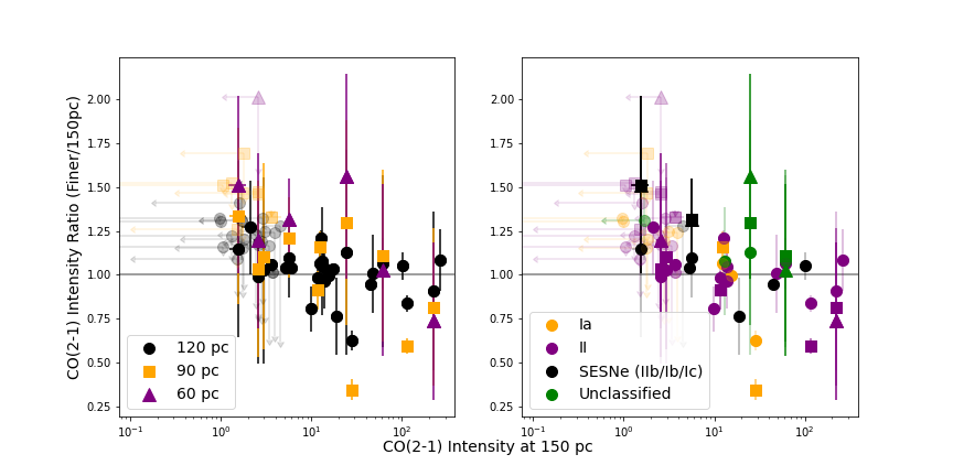
In Figure 7, we focus directly on the sites of SN explosions with measurements at multiple resolutions. In both panels, we compare the intensity of CO (2-1) emission measured at 150 pc resolution to the ratio of the CO (2-1) emission intensity measured at finer resolution to the 150 pc measurement for each SNe site with a 60, 90, or 120 pc resolution map. Non-detections that are assigned upper-limit values are plotted with transparent markers and with error-bar-length arrows. Points that are in vertical alignment – that have the same -axis value for each resolution – are taken from the same SN site. By design, the upper-limit measurements (transparent markers) that have vertical alignment will have increased intensity at higher resolutions because the noise increases at resolutions finer than 150 pc. In the left panel we consider all of the SN sites, in the right panel we differentiate our sample by SN type.
For the points that have CO (2-1) detections, the plot shows mixed results. Some of our SN sample show increased intensity at finer resolution, implying that they are directly associated with molecular gas that was partially “smoothed out” at coarser resolution. Others show a decrease in intensity, implying that at least a portion of the measured molecular gas coincident with the SN at 150 pc is not centrally located at the SN’s explosion site. Overall, there appears to be a trend that the SNe with lowest intensity at 150 pc resolution show at least a moderate increase in intensity at finer resolution, suggesting that the SNe are near to or within molecular clouds in these regions.
Separating the sample by SN type we find mixed results, with all except for the unclassified population exhibiting cases of both increasing and decreasing intensity ratios at higher resolutions. The unclassified sample does show consistently higher CO (2-1) emission intensities at higher resolutions, which perhaps reflects the difficulty in obtaining spectra for classification in high extinction regions. This plot shows that the local environments of our SNe are varied and accounting for their feedback is complicated. This also speaks to the importance of pursuing these environments with even higher resolution observations in the future.
III.4 CO (2-1) Distributions Around the Sites of Individual SNe
So far we have considered only emission directly at the location of the SNe, but the position of the SNe relative to nearby CO (2-1) emission may also hold important information. As a final exercise, we explore the spatial distribution of CO (2-1) near our SNe. To do this, in this section with construct cutout images using the highest resolution CO (2-1) map for each SNe and in §III.5 we analyze the distance from each SNe to the nearest molecular gas detection.
Figure 8 shows cutouts of each of the 59 SN explosion sites that have CO (2-1) maps with at least 150 pc resolution. These “zoom in” images allow us to visually locate the SN explosion sites relative to the nearby molecular gas. Inspecting the images, we explore whether the SNe with CO (2-1) detection are located towards the peaks of the CO (2-1) emission, or if they lie off to the side, sharing space with an MC that just happens to be caught in the beam. This latter case might arise if the SNe drifted away from their parent cloud or if other forms of feedback or previous SNe already dispersed the parent cloud. Similarly, we can inspect whether SNe with non-detections might have nearby molecular gas that is just not directly coincident with the SNe.
Examining the maps, we note several impressions. First, we find 100% agreement between the detection classification at 150 pc and at those at finer resolutions from (60-120 pc). Second, the cutouts show that the molecular gas around the SNe is often extended at the resolution shown and sometimes patchy. Non-detections often lie in the vicinity of CO (2-1) emission. Detections are often not on the emission peaks themselves but off to the side. Overall, the zooms show that the SNe are exploding into environments that have a wide range of molecular gas densities and landscapes and tend to show a high degree of local variation in density.
We study recent SNe that have not yet affected their environments. We plot three “spheres of future influence” in order to estimate the size of the region they will affect in the future and so form an idea of how these explosions may change the nearby ISM. White circles show apertures with radii of 6.3, 32, and 203 pc around each SNe site. The 6.3 pc aperture is an estimate of the cooling radius88 8 The cooling radius is the spatial scale over which the ISM receives a significant momentum boost from the SN explosion (i.e. momentum feedback), as confirmed by recent simulations (Martizzi et al. 2015; Kim & Ostriker 2015, e.g.,). During this time, radiative losses become important during the evolution of the SNR. of an SNR in the turbulent and inhomogeneous ISM at a typical molecular gas density () (Martizzi et al. 2015). The 32 and 203 pc apertures represent the cooling and fadeaway99 9 The fadeaway radius is the physical point where the shock front of the SNR slows to match the surrounding ISM’s effective sound speed. radii for a SNR in low-density () environments (Draine 2011). Although the actual radii are dependent on the exact density structure of the ISM and the energy of the SN, these estimates allow us to visualize how much of the surrounding ISM could be influenced by the SNe that have just exploded.
Inspecting the individual SN sites in Figure 8 we identify five general cases:
- 1.
Non-detections with CO (2-1) within the cooling radius. A few of the CO (2-1) non-detections show nearby emission that suggests future interaction between the SN and the nearby molecular gas. Specifically, 7% (4/59) of the panels show the presence of molecular gas within the low-density cooling radius of a non-detection classification. Specific SNe: SN1935C, SN2016cok, SN1964F, & SN2007it.
- 2.
Non-detections with CO (2-1) within the fadeaway radius. An additional 24% (14/59) show molecular gas within the fadeaway radius of a non-detection classification. We expect these SN to be likely to interact with the surrounding ISM sometime before fading, though the interaction may be relatively weaker than for the first group of non-detections. Specific SNe: SN1985P, SN2006ov, SN2014dt, SN2006X, SN2019ehk, SN1960F, SN1981B, SN2008bk, SN2013ej, SN2001du, SN1986L, SN1993Z, SN2020jfo, & SN1979C.
- 3.
Detections with nearby voids or low-density regions. 8% (5/59) of our sample show CO (2-1) detections but also the presence of nearby voids or lower-density regions on the edge or just outside the high-density cooling radius at our detection classifications. We expect the explosion blast wave to move more quickly through these lower-density regions, while slowing through interaction with the denser ISM in the higher-density areas. Specific SNe: SN2009ib, SN1972Q, SN1923A, SN1983N, & SN2005at.
- 4.
Detections in regions with widespread high surface densities. 47% (28/59) occur in apparently dense regions where CO (2-1) emission extends completely past the high-density cooling radius. These are the most likely cases for the the energy of the SN to contribute to the destruction or reshaping of the nearby MCs without breaking through to the surrounding low-density ISM. We caution however that the three-dimensional distribution and substructure below our resolution remain unknown, so even these cases may still have low-density channels through which some of the explosion can exert a more extended effect. Specific SNe: SN1996cr, SN1940E, SN1995V, SN1992bd, SN1983V, SN1984J, ASASSN-14ha, SN2010el, SN1999em, SN2003jg, SN2008eh, SN1973R, SN1989B, SN2009hd, SN1967H, SN1986I, SN2014L, SN1999gn, SN1901B, SN1959E, SN2020oi, SN2020nvb, SN2011ja, SN1986G, SN2016adj, SN1950B, SN1957D, & SN1968L.
- 5.
Non-detections with little or no nearby molecular gas. The remaining 14% (8/59) occur isolated from nearby detected molecular gas extending all the way past the low-density fadeaway radius. These SNe are the most likely ones to drive turbulence in the atomic gas, carve out large bubbles and shells, potentially launch outflows, and otherwise interact primarily with the diffuse ISM. Specific SNe: SN1999eu, SN2012fr, SN2005df, SN2012A, SN1926A, SN1961I, SN2012cg, & SN1988M.


| Case | Total SNe | SN Ia | SN II | SESNe | Unclassified |
|---|---|---|---|---|---|
| 1. Non-detections with SNe within cooling radius | 4 | 0 | 3 | 0 | 1 |
| 2. Non-detections with SNe within fadeaway radius | 14 | 5 | 8 | 1 | 0 |
| 3. Detections with nearby voids | 5 | 0 | 3 | 2 | 0 |
| 4. Detections in widespread high surface density | 28 | 4 | 14 | 4 | 6 |
| 5. Non-detections with no nearby CO | 8 | 3 | 5 | 0 | 0 |
Table III.4 shows the SN type distribution among the five different cutout cases described above. Cases 1, 2, and 5 represent environments with the lowest amounts of nearby molecular gas. Case 1 is predominantly SNe II while Cases 2 and 5 have the highest fraction of SNe Ia compared to the other cases. In Case 1 we find predominantly SNe II that do not have strong enough CO (2-1) emission to be considered a detection, yet they have molecular gas coincident within parsecs. This is consistent with CCSNe progenitors with lifetimes on the order of s of Myrs that will have time to migrate some distance away from their parent cloud before exploding. Cases 2 and 5 represent the SN environments most devoid of molecular gas and host the highest fractions of SNe Ia and SNe II. Collectively, Cases 1, 2, and 5 support the weakest association between molecular gas and SNe Ia and II. Cases 3 and 4 host 86% (6/7) of the total SESNe and unclassified SNe populations and clearly show that these are more associated with the highest molecular gas surface density regions. This is consistent with SESNe originating from some of the most massive progenitors and having the shortest lifetimes.
Even more than the statistical analysis, the cutouts clearly show that even in gas-rich regions of massive galaxies, SNe must play a varied role in exerting feedback on their surrounding environment, occurring across a wide range of molecular gas densities. Given the patchy gas distribution and the position of the SNe near both high- and low-column density regions, most of our SNe (even many of our non-detections) may both plausibly interact with molecular gas in the future and have a channel to affect the lower-density, diffuse ISM. It seems likely that individual SNe, many of which lie near the edges of molecular structures, play multiple roles, both affecting the dense and diffuse ISM.
III.5 Distance from SNe to the nearest detected molecular gas
Finally, as a quantitative complement to §III.4, we measure the distance from each SNe to the nearest pixel with well-detected molecular gas at each galaxy’s individual median value. These values range from 3.6 to 17 with a median value of 7.9. We compare these measured distances for our real SN sample to four model populations, each constructed to reflect a distinct hypothesis for where SNe explode in our targets. Figure 9 shows how we generate these model SNe populations. The four hypotheses are:

- 1.
Purely random: the SN distribution is completely random with SNe equally likely to occur in each pixel of the map. This would be a fitting model if SNe simply occurred randomly in space with no relation to their parent galaxy. This is not expected but represents the simplest control, so we calculate it.
- 2.
Following the molecular gas distribution: the SN distribution favors pixels at local peaks in the density field. We assign a probability that a SN will occur at a given pixel based on the intensity profile of the PHANGS–ALMA CO (2-1) maps. This would be expected if the gas distribution is long-lived in its current configuration, the amount of gas determines the amount of star formation, and the SNe overall trace the locations of star formation. Because CCSNe trace high-mass star formation and high-mass star formation follows the molecular gas, we expect this to be a good general model for the placement of CCSNe. This model will be biased to preferentially place SNe in galaxy centers, although, observationally, SN are difficult to observe in these dense, bright regions, leaving our real SN sample with fewer SNe from these regions.
- 3.
Following the stellar disk: the SN distribution follows the distribution of stellar mass in the galaxy, which tends to be smoother than the gas distribution and overall resembles an exponential disk in most targets. We assign a probability that a SN will occur at a given pixel based on the intensity profile of the near-IR maps described in §II. Type Ia SNe have been shown to follow the stellar disk (Maoz et al. 2014; Anderson et al. 2015a; Cronin et al. 2021). For this reason, we would expect this model to provide good placement for Type Ia SNe.
- 4.
Hybrid model: We combine the two previous models, generating 24% of our SN population to occur following the stellar disk and 76% following the gas distribution. This ratio is set from previous work that has shown that for massive star forming galaxies 24% of observed SNe are Type Ia (Li et al. 2011), which closely resembles our SNe population of 23% SNe Ia.
We generate 100 model SNe for each galaxy in our sample for which we have a map at 150 pc resolution1010 10 missing 150 pc CO (2-1) maps for NGC 1068, 1672, and 4579. This gives us a total of 2900 model SNe from 29 galaxies generated for each of the four models.

In Figure 10 we show the cumulative distributions of the distances to the nearest pixel with each galaxy’s individual median value for both our real SN sample (59 SNe) and each of our four model SN populations (2900 SNe generated for each model). In the top panel we plot our real SN sample together regardless of type, in the bottom panel we separate our real SN sample by type. In the top panel of Figure 10, the random model produces very unrealistic results, with little or no association between the SNe and CO (2-1) emission. On the other hand, the distribution following gas directly produces too close of an association. The hybrid model does significantly better, with the observations producing a distance distribution between the stellar disk model at small distances and the hybrid model at larger distances. We find that almost of our SN sample is within 100 pc of a molecular gas surface density of our value of or higher. In the bottom panel of Figure 10 we find that the SESNe and untyped SNe are found close to well-detected molecular gas, with 100% of our SNe Ibc and 85% of our untyped SNe occurring with a CO (2-1) detection within the beam at 150 pc. Approximately 60% of our SNe II occur with CO (2-1) detection in the beam with occurring within 300 pc of molecular gas. SNe Ia tend to be found at a wider range of distances to molecular gas with occurring with a CO (2-1) detection in the beam with occurring within 400 pc of molecular gas.

Figure 11 is constructed similarly to Figure 10 but instead we show the cumulative distributions of the mass as a function of the molecular gas surface density at the locations of our SN sample at 150 pc resolution for both our real SNe sample (59 SNe) and each of our four model SNe populations (2900 SNe in each model). We find that the CDF of our observed SNe sample lies between the stellar disk model and the hybrid model, but more closely follows the stellar disk model. In the bottom panel we separate the observed SNe by type and repeat the comparison. We find the SNe Ia and II more closely follow the random and stellar disk model respectively, the SNe Ibc more closely follow between the stellar disk model and the hybrid model, and the unclassified SNe more closely follow the hybrid model.
IV Discussion and Conclusions
We perform the first statistical characterization of the molecular gas content at the location of SN explosion sites on pc scales. This is the first time an observational study on feedback from individual SNe has been done on the scales of individual GMCs.
The effects of SNe on their host galaxies are location dependent. If a SN explodes within an MC, its energy and momentum may work to disperse that cloud. On larger scales, SN explosions may collect and compress gas, helping to trigger star formation. And if a SN explodes in the diffuse ISM, the explosion may be well-placed to create turbulence in diffuse gas or launch galactic winds or fountains.
Until recently, it was not possible to measure the gas content of SN explosion sites at resolutions high enough to associate individual explosions with gas likely to interact with that SN. Thanks to large samples of SN discoveries and new high-resolution CO (2-1) surveys with ALMA, this situation is changing.
We measure the CO (2-1) emission from the sites of recent ( years) SNe, which allows us to place SN explosions in the context of their host galaxies and investigate the role that feedback from these explosions could play in the evolution of GMCs.
- 1.
We identified 63 SNe from the OSC that exploded in 31 galaxies from the PHANGS-ALMA footprint (see Figure 1c and Table ). We measure the CO (2-1) intensity at the SN locations across a wide range of resolutions from 60 pc to 1 kpc (see Table Comparing the Locations of Supernovae to CO (2-1) Emission in their Host Galaxies). We find that of our SN explosion sites have detectable CO (2-1) emission on 1 kpc scales and on 150 pc scales (see §III.1, Figure 2: Table III.1, and Table III.3). Primarily this difference between results at different scales appears to reflect that SNe explode in gas-rich regions of galaxies but that they do not always appear directly coincident with gas peaks at higher resolution. This is reinforced by Figure 8, where we zoom-in to the immediate environment of each of our SNe and find that most of them occur off-peak of the nearby molecular gas.
- 2.
We construct a working sample of 59 SNe that have CO (2-1) intensity measurements at 150pc resolution (see §III.2). We compare distributions of molecular gas surface densities at the sites of these SN explosions to the overall distributions in the PHANGS–ALMA CO (2-1) maps. We find that SNe consistently explode in regions with higher than average molecular gas surface densities (see Figure 3, Figure 4, and Table III.2.2). We find this despite the fact that one might expect optical SN searches to be biased against SN that occur in the most gas-rich parts of galaxies due to the effects of extinction.
- 3.
When separating our SN sample by type, we find that our CCSNe (SNe II and SESNe – IIb/Ib/Ic) occur in brighter CO (2-1) emitting regions than our SNe Ia (see Figure 4 and Table III.2.2). Our sample of SESNe show the strongest association with bright CO (2-1) emission, and have the highest fraction of CO (2-1) detections of all SN types occurring in the galaxies’ highest density regions. In turn, SNe II have a stronger association with CO (2-1) emission than SNe Ia. Taking these results together, we find an SN’s association with peaks in molecular gas density to decrease as a function of progenitor mass (see Figure 5). We find that the unclassified SNe are most consistent with the SESNe population (see Figure 4 and Figure 11), with of the unclassified SNe coincident with dense GMCs (see Figure 8). It is possible that spectroscopic follow-ups of transients could miss SESNe in regions with high extinction.
- 4.
We plot CO (2-1) emission in a local region centered on each SN in our sample in order to visually inspect the SN location (see Figure 8). The images show that even when CO (2-1) is detected SNe often occur displaced from the local peak of CO (2-1) emission, and the surrounding region often shows a wide range of molecular gas surface densities. Meanwhile, a significant fraction of SNe with non-detections have some nearby CO (2-1) that might plausibly interact with the SN explosion before it fades away.
- 5.
Finally, we model four different populations of SN locations and compare their distributions with that of our observations (see Figure 9). We find that CDFs of both the distance to the nearest well-detected molecular gas and the surrounding molecular gas surface density of our observed SN sample falls between the locations of modeled SNe generated to follow the infrared emission of older stellar populations and the locations of SNe generated to follow a hybrid model with molecular gas and stellar infrared emission. (see §III.5: Figure 10 and Figure 11).
These results show that the molecular gas landscape in the vicinity of recent SNe is varied, and we can expect that the impact of a SN on its local environment has the potential to be complex. This speaks to the importance of having high-resolution measurements to better describe these environments in the future.
We expect that both the SN sample and the gas data used for this study will improve over the next few years. We use a SN sample drawn from heterogeneous observations over the last century, and these observations often have unknown completeness and biases against finding SNe in dusty, high-extinction regions like MCs or galaxy centers.
Systematic surveys that image the entire sky at high cadence – such as the All Sky Automated Search for SN (Shappee et al. 2014; Kochanek et al. 2017, ASAS-SN,) and the Vera C. Rubin Observatory’s Legacy Survey of Space and Time (Cook et al. 2004, LSST,) are changing this. Over time we expect large highly complete samples of SNe to emerge for nearby galaxies. Future SN environment studies will benefit from these surveys.
Although this work provides us an up-close view of a SN environment on a 100 pc scale, further advances will come from exploring these regions on even smaller, sub-MC, scales: CO (2-1) observations can plausibly be pushed to resolutions of pc, enough to cleanly locate the SN relative to any MCs and resolve the future cooling radius or region of likely interaction. There are also gains to be made by improving the sensitivity. Our point-mass sensitivity for much of the survey corresponds to the mass of an individual GMC, but we cannot rule out the presence of lower-mass clouds. With deeper integration we could ascertain whether or not a lower-mass cloud is present.
Future directions include looking at CO (2-1) emission line widths to explore if the explosions are well-placed to add turbulence to diffuse gas or to launch galactic winds or fountains, as well as looking at H emission to see how often the SNe visibly reside in regions cleared by pre-SN feedback.
ADS/JAO.ALMA#2012.1.00650.S
ADS/JAO.ALMA#2013.1.00803.S
ADS/JAO.ALMA#2013.1.01161.S
ADS/JAO.ALMA#2015.1.00121.S
ADS/JAO.ALMA#2015.1.00782.S
ADS/JAO.ALMA#2015.1.00925.S
ADS/JAO.ALMA#2015.1.00956.S
ADS/JAO.ALMA#2016.1.00386.S
ADS/JAO.ALMA#2017.1.00392.S
ADS/JAO.ALMA#2017.1.00766.S
ADS/JAO.ALMA#2017.1.00886.L
ADS/JAO.ALMA#2018.1.00484.S
ADS/JAO.ALMA#2018.1.01321.S
ADS/JAO.ALMA#2018.1.01651.S
ADS/JAO.ALMA#2018.A.00062.S
ADS/JAO.ALMA#2019.1.01235.S
ADS/JAO.ALMA#2019.2.00129.S
ALMA is a partnership of ESO (representing its member states), NSF (USA), and NINS (Japan), together with NRC (Canada), NSC and ASIAA (Taiwan), and KASI (Republic of Korea), in cooperation with the Republic of Chile. The Joint ALMA Observatory is operated by ESO, AUI/NRAO, and NAOJ. The National Radio Astronomy Observatory (NRAO) is a facility of NSF operated under cooperative agreement by Associated Universities, Inc (AUI). This work acknowledges the Open Supernova Catalog (OSC; Guillochon et al. 2017), last accessed on 2021 May 25, which included observations and metadata for 80,000 SNe & SNRs. This work has made use of SAO/NASA Astrophysics Data System1111 11 http://www.adsabs.harvard.edu, the NASA/IPAC Extragalactic Database (NED), which is operated by the Jet Propulsion Laboratory, California Institute of Technology, under contract with the National Aeronautics and Space Administration, and the SIMBAD database, operated at CDS, Strasbourg, France. This work has utilized the following software: Jupyter (Kluyver et al. 2016), Astropy (Astropy Collaboration et al. 2013; Astropy Collaboration et al. 2018), Pandas (Wes McKinney 2010), NumPy (van der Walt et al. 2011; Harris et al. 2020), SciPy (Virtanen et al. 2020), Seaborn (Waskom et al. 2017), Matplotlib (Hunter 2007), & GitHub (github 2020).
References
- Aadland et al. (2018) Aadland, E., Massey, P., Neugent, K. F., & Drout, M. R. 2018, AJ, 156, 294
- Accurso et al. (2017) Accurso, G., Saintonge, A., Catinella, B., et al. 2017, MNRAS, 470, 4750
- Adamo et al. (2020) Adamo, A., Zeidler, P., Kruijssen, J. M. D., et al. 2020, Space Sci. Rev., 216, 69
- Adams & Kochanek (2015) Adams, S. M., & Kochanek, C. S. 2015, MNRAS, 452, 2195
- Anderson et al. (2012) Anderson, J. P., Habergham, S. M., James, P. A., & Hamuy, M. 2012, MNRAS, 424, 1372
- Anderson & James (2008) Anderson, J. P., & James, P. A. 2008, MNRAS, 390, 1527
- Anderson & James (2009) —. 2009, MNRAS, 399, 559
- Anderson et al. (2015a) Anderson, J. P., James, P. A., Förster, F., et al. 2015a, MNRAS, 448, 732
- Anderson et al. (2015b) Anderson, J. P., James, P. A., Habergham, S. M., Galbany, L., & Kuncarayakti, H. 2015b, PASA, 32, e019
- Andersson et al. (2020) Andersson, E. P., Agertz, O., & Renaud, F. 2020, MNRAS, 494, 3328
- Andreoni & Goldstein (2019a) Andreoni, I., & Goldstein, D. 2019a, Transient Name Server Discovery Report, 2019-1496, 1
- Andreoni & Goldstein (2019b) —. 2019b, Transient Name Server Discovery Report, 2019-1507, 1
- Andreoni & Goldstein (2019c) —. 2019c, Transient Name Server Discovery Report, 2019-1677, 1
- Andrews et al. (2019) Andrews, J., Valenti, S., Lundquist, M., et al. 2019, Transient Name Server Classification Report, 2019-1920, 1
- Andrews et al. (2021) Andrews, J. E., Jencson, J. E., Van Dyk, S. D., et al. 2021, ApJ, 917, 63
- Arcavi et al. (2014) Arcavi, I., Valenti, S., Hosseinzadeh, G., et al. 2014, The Astronomer’s Telegram, 6466, 1
- Astropy Collaboration et al. (2013) Astropy Collaboration, Robitaille, T. P., Tollerud, E. J., et al. 2013, A&A, 558, A33
- Astropy Collaboration et al. (2018) Astropy Collaboration, Price-Whelan, A. M., Sipőcz, B. M., et al. 2018, AJ, 156, 123
- Audcent-Ross et al. (2020) Audcent-Ross, F. M., Meurer, G. R., Audcent, J. R., et al. 2020, MNRAS, 492, 848
- Ayani & Yamaoka (1999) Ayani, K., & Yamaoka, H. 1999, IAU Circ., 7336, 1
- Barbon et al. (1973) Barbon, R., Ciatti, F., & Rosino, L. 1973, A&A, 29, 57
- Barnes et al. (2021) Barnes, A. T., Glover, S. C. O., Kreckel, K., et al. 2021, MNRAS, 508, 5362
- Beasor et al. (2021) Beasor, E. R., Davies, B., Smith, N., Gehrz, R. D., & Figer, D. F. 2021, ApJ, 912, 16
- Benincasa et al. (2020) Benincasa, S. M., Loebman, S. R., Wetzel, A., et al. 2020, MNRAS, 497, 3993
- Bessell & Schmidt (2010) Bessell, M. S., & Schmidt, B. P. 2010, Central Bureau Electronic Telegrams, 2337, 1
- Blondin et al. (2006) Blondin, S., Modjaz, M., Kirshner, R., Challis, P., & Berlind, P. 2006, Central Bureau Electronic Telegrams, 757, 1
- Bolatto et al. (2013) Bolatto, A. D., Wolfire, M., & Leroy, A. K. 2013, ARA&A, 51, 207
- Bolatto et al. (2017) Bolatto, A. D., Wong, T., Utomo, D., et al. 2017, ApJ, 846, 159
- Busko et al. (1981) Busko, I., Jablonski, F., Torres, C., Wood, R., & Clements, E. D. 1981, IAU Circ., 3580, 2
- Buta (1984) Buta, R. 1984, IAU Circ., 3967, 2
- Cao et al. (2012) Cao, Y., Kasliwal, M. M., Wallerstein, G., Ritchey, A., & Howell, D. A. 2012, The Astronomer’s Telegram, 3855, 1
- Carney (1980) Carney, B. W. 1980, PASP, 92, 56
- Chambers et al. (2019) Chambers, K. C., Boer, T. D., Bulger, J., et al. 2019, Transient Name Server Discovery Report, 2019-1014, 1
- Chevalier & Clegg (1985) Chevalier, R. A., & Clegg, A. W. 1985, Nature, 317, 44
- Chevance et al. (2020) Chevance, M., Kruijssen, J. M. D., Hygate, A. P. S., et al. 2020, MNRAS, 493, 2872
- Chevance et al. (2022) Chevance, M., Kruijssen, J. M. D., Krumholz, M. R., et al. 2022, MNRAS, 509, 272
- Choi et al. (2017) Choi, J., Conroy, C., & Byler, N. 2017, ApJ, 838, 159
- Ciatti & Rosino (1977) Ciatti, F., & Rosino, L. 1977, A&A, 56, 59
- Contreras et al. (2007) Contreras, C., Morrell, N., Gonzalez, S., & Lee, K. G. 2007, Central Bureau Electronic Telegrams, 1068, 1
- Cook et al. (2004) Cook, K. H., Saha, A., Pierfedrici, F., et al. 2004, in American Astronomical Society Meeting Abstracts, Vol. 205, American Astronomical Society Meeting Abstracts, 108.09
- Corbelli et al. (2017) Corbelli, E., Braine, J., Bandiera, R., et al. 2017, A&A, 601, A146
- Cronin et al. (2021) Cronin, S. A., Utomo, D., Leroy, A. K., et al. 2021, ApJ, 923, 86
- De et al. (2021) De, K., Fremling, U. C., Gal-Yam, A., et al. 2021, ApJ, 907, L18
- den Brok et al. (2021) den Brok, J. S., Chatzigiannakis, D., Bigiel, F., et al. 2021, MNRAS, 504, 3221
- Dobbs & Pringle (2013) Dobbs, C. L., & Pringle, J. E. 2013, MNRAS, 432, 653
- Draine (2011) Draine, B. T. 2011, Physics of the Interstellar and Intergalactic Medium
- Evans & McNaught (2003) Evans, R., & McNaught, R. H. 2003, IAU Circ., 8150, 2
- Evans et al. (1995) Evans, R. O., Jarman, J., Cragg, T., et al. 1995, IAU Circ., 6197, 2
- Fairall (1972) Fairall, A. P. 1972, Monthly Notes of the Astronomical Society of South Africa, 31, 23
- Filippenko & Foley (2005) Filippenko, A. V., & Foley, R. J. 2005, IAU Circ., 8484, 2
- Filippenko & Sargent (1988) Filippenko, A. V., & Sargent, W. L. W. 1988, IAU Circ., 4591, 2
- Fox et al. (2021) Fox, O. D., Khandrika, H., Rubin, D., et al. 2021, MNRAS, 506, 4199
- Fukui & Kawamura (2010) Fukui, Y., & Kawamura, A. 2010, ARA&A, 48, 547
- Galbany et al. (2012) Galbany, L., Miquel, R., Östman, L., et al. 2012, ApJ, 755, 125
- Galbany et al. (2014) Galbany, L., Stanishev, V., Mourão, A. M., et al. 2014, A&A, 572, A38
- Galbany et al. (2017) Galbany, L., Mora, L., González-Gaitán, S., et al. 2017, MNRAS, 468, 628
- Gaskell et al. (1986) Gaskell, C. M., Cappellaro, E., Dinerstein, H. L., et al. 1986, ApJ, 306, L77
- Gatto et al. (2017) Gatto, A., Walch, S., Naab, T., et al. 2017, MNRAS, 466, 1903
- Geen et al. (2016) Geen, S., Hennebelle, P., Tremblin, P., & Rosdahl, J. 2016, MNRAS, 463, 3129
- Gies (1987) Gies, D. R. 1987, ApJS, 64, 545
- github (2020) github. 2020, GitHub
- Grasha et al. (2018) Grasha, K., Calzetti, D., Bittle, L., et al. 2018, MNRAS, 481, 1016
- Grasha et al. (2019) Grasha, K., Calzetti, D., Adamo, A., et al. 2019, MNRAS, 483, 4707
- Green (2019) Green, D. A. 2019, Journal of Astrophysics and Astronomy, 40, 36
- Guillochon et al. (2017) Guillochon, J., Parrent, J., Kelley, L. Z., & Margutti, R. 2017, ApJ, 835, 64
- Habergham et al. (2010) Habergham, S. M., Anderson, J. P., & James, P. A. 2010, ApJ, 717, 342
- Habergham et al. (2012) Habergham, S. M., James, P. A., & Anderson, J. P. 2012, MNRAS, 424, 2841
- Harris et al. (2020) Harris, C. R., Millman, K. J., van der Walt, S. J., et al. 2020, Nature, 585, 357
- Ho (2019) Ho, A. 2019, Transient Name Server Discovery Report, 2019-1165, 1
- Holoien et al. (2019) Holoien, T. W. S., Brown, J. S., Vallely, P. J., et al. 2019, MNRAS, 484, 1899
- Howell (2003) Howell, D. A. 2003, IAU Circ., 8241, 2
- Hunter (2007) Hunter, J. D. 2007, Computing in Science & Engineering, 9, 90
- Iffrig & Hennebelle (2015) Iffrig, O., & Hennebelle, P. 2015, A&A, 576, A95
- James & Anderson (2006) James, P. A., & Anderson, J. P. 2006, A&A, 453, 57
- Jencson et al. (2019) Jencson, J. E., Kasliwal, M. M., Adams, S. M., et al. 2019, ApJ, 886, 40
- Jencson et al. (2021) Jencson, J. E., Andrews, J. E., Bond, H. E., et al. 2021, ApJ, 920, 127
- Jha et al. (1999) Jha, S., Challis, P., Garnavich, P., et al. 1999, IAU Circ., 7296, 2
- Jha et al. (2017) Jha, S. W., Camacho, Y., Dettman, K., et al. 2017, The Astronomer’s Telegram, 10640, 1
- Jiang et al. (2010) Jiang, B., Chen, Y., Wang, J., et al. 2010, ApJ, 712, 1147
- Kandrashoff et al. (2012) Kandrashoff, M., Cenko, S. B., Li, W., et al. 2012, Central Bureau Electronic Telegrams, 3111, 1
- Kangas et al. (2013) Kangas, T., Mattila, S., Kankare, E., et al. 2013, MNRAS, 436, 3464
- Kasliwal et al. (2009) Kasliwal, M. M., Sahu, D. K., & Anupama, G. C. 2009, Central Bureau Electronic Telegrams, 1874, 2
- Kasliwal et al. (2017) Kasliwal, M. M., Bally, J., Masci, F., et al. 2017, ApJ, 839, 88
- Kawamura et al. (2009) Kawamura, A., Mizuno, Y., Minamidani, T., et al. 2009, ApJS, 184, 1
- Keller & Kruijssen (2020) Keller, B. W., & Kruijssen, J. M. D. 2020, arXiv e-prints, arXiv:2004.03608
- Keller et al. (2022) Keller, B. W., Kruijssen, J. M. D., & Chevance, M. 2022, MNRAS, arXiv:2206.06391
- Kelly et al. (2008) Kelly, P. L., Kirshner, R. P., & Pahre, M. 2008, ApJ, 687, 1201
- Kendurkar (2018) Kendurkar, M. R. 2018, Transient Name Server Discovery Report, 2018-1093, 1
- Kharadze et al. (1989) Kharadze, E. K., Pskovsky, Y. P., Kimeridze, G. N., et al. 1989, IAU Circ., 4802, 1
- Kilpatrick et al. (2016) Kilpatrick, C. D., Bieging, J. H., & Rieke, G. H. 2016, ApJ, 816, 1
- Kim & Ostriker (2015) Kim, C.-G., & Ostriker, E. C. 2015, ApJ, 802, 99
- Kim et al. (2021) Kim, J., Chevance, M., Kruijssen, J. M. D., et al. 2021, MNRAS, 504, 487
- Kim et al. (2022) —. 2022, arXiv e-prints, arXiv:2206.09857
- Kim et al. (2018) Kim, J.-G., Kim, W.-T., & Ostriker, E. C. 2018, ApJ, 859, 68
- Kirshner et al. (1985) Kirshner, R., Schild, R., Wilson, I. R. G., Buta, R., & Meurer, G. 1985, IAU Circ., 4143, 1
- Klotz et al. (2012) Klotz, A., Maury, A., Childress, M., et al. 2012, Central Bureau Electronic Telegrams, 3275, 1
- Kluyver et al. (2016) Kluyver, T., Ragan-Kelley, B., Pérez, F., et al. 2016, in IOS Press, 87–90
- Kochanek et al. (2017) Kochanek, C. S., Shappee, B. J., Stanek, K. Z., et al. 2017, PASP, 129, 104502
- Kosai et al. (1988) Kosai, H., Ikeya, K., Evans, R. O., et al. 1988, IAU Circ., 4533, 1
- Kruijssen (2012) Kruijssen, J. M. D. 2012, MNRAS, 426, 3008
- Kruijssen et al. (2019) Kruijssen, J. M. D., Schruba, A., Chevance, M., et al. 2019, Nature, 569, 519
- Krumholz & Matzner (2009) Krumholz, M. R., & Matzner, C. D. 2009, ApJ, 703, 1352
- Krumholz et al. (2019) Krumholz, M. R., McKee, C. F., & Bland-Hawthorn, J. 2019, ARA&A, 57, 227
- Leitherer et al. (2014) Leitherer, C., Ekström, S., Meynet, G., et al. 2014, ApJS, 212, 14
- Leroy et al. (2019) Leroy, A. K., Sandstrom, K. M., Lang, D., et al. 2019, ApJS, 244, 24
- Leroy et al. (2021a) Leroy, A. K., Rosolowsky, E., Usero, A., et al. 2021a, arXiv e-prints, arXiv:2109.11583
- Leroy et al. (2021b) Leroy, A. K., Schinnerer, E., Hughes, A., et al. 2021b, arXiv e-prints, arXiv:2104.07739
- Li et al. (2011) Li, W., Leaman, J., Chornock, R., et al. 2011, MNRAS, 412, 1441
- Lloyd Evans et al. (1986) Lloyd Evans, T., Evans, R., & McNaught, R. H. 1986, IAU Circ., 4262, 2
- Lopez et al. (2011) Lopez, L. A., Krumholz, M. R., Bolatto, A. D., Prochaska, J. X., & Ramirez-Ruiz, E. 2011, ApJ, 731, 91
- Lopez et al. (2014) Lopez, L. A., Krumholz, M. R., Bolatto, A. D., et al. 2014, ApJ, 795, 121
- Lopez et al. (2020) Lopez, L. A., Mathur, S., Nguyen, D. D., Thompson, T. A., & Olivier, G. M. 2020, ApJ, 904, 152
- Lu et al. (2020) Lu, Z.-J., Pelkonen, V.-M., Padoan, P., et al. 2020, ApJ, 904, 58
- Lucas et al. (2020) Lucas, W. E., Bonnell, I. A., & Dale, J. E. 2020, MNRAS, 493, 4700
- Maoz & Graur (2017) Maoz, D., & Graur, O. 2017, ApJ, 848, 25
- Maoz et al. (2014) Maoz, D., Mannucci, F., & Nelemans, G. 2014, ARA&A, 52, 107
- Marples & Bock (2016) Marples, P., & Bock, G. 2016, Transient Name Server Discovery Report, 2016-94, 1
- Martin et al. (2005) Martin, R., Yamaoka, H., Monard, L. A. G., & Africa, S. 2005, Central Bureau Electronic Telegrams, 119, 1
- Martizzi et al. (2015) Martizzi, D., Faucher-Giguère, C.-A., & Quataert, E. 2015, MNRAS, 450, 504
- Martizzi et al. (2016) Martizzi, D., Fielding, D., Faucher-Giguère, C.-A., & Quataert, E. 2016, MNRAS, 459, 2311
- Marvin et al. (1989) Marvin, H., Perlmutter, S., Seal, D., et al. 1989, IAU Circ., 4727, 1
- Maza et al. (1999) Maza, J., Hamuy, M., Antezana, R., et al. 1999, IAU Circ., 7210, 1
- McKee & Ostriker (1977) McKee, C. F., & Ostriker, J. P. 1977, ApJ, 218, 148
- McLeod et al. (2020) McLeod, A. F., Kruijssen, J. M. D., Weisz, D. R., et al. 2020, ApJ, 891, 25
- McLeod et al. (2021) McLeod, A. F., Ali, A. A., Chevance, M., et al. 2021, MNRAS, 508, 5425
- Meidt et al. (2015) Meidt, S. E., Hughes, A., Dobbs, C. L., et al. 2015, ApJ, 806, 72
- Monard (2008a) Monard, L. A. G. 2008a, Central Bureau Electronic Telegrams, 1315, 1
- Monard (2008b) —. 2008b, Central Bureau Electronic Telegrams, 1445, 1
- Monard et al. (2011) Monard, L. A. G., Milisavljevic, D., Fesen, R., et al. 2011, Central Bureau Electronic Telegrams, 2946, 1
- Morrell & Stritzinger (2008) Morrell, N., & Stritzinger, M. 2008, Central Bureau Electronic Telegrams, 1335, 1
- Müller (2016) Müller, B. 2016, PASA, 33, e048
- Murray et al. (2010) Murray, N., Quataert, E., & Thompson, T. A. 2010, ApJ, 709, 191
- Nakano & Aoki (1999) Nakano, S., & Aoki, M. 1999, IAU Circ., 7304, 2
- Ochner et al. (2018) Ochner, P., Pastorello, A., Campaner, P., De Biasi, L., & Rossi, M. 2018, The Astronomer’s Telegram, 12239, 1
- Ochner et al. (2014) Ochner, P., Tomasella, L., Benetti, S., et al. 2014, Central Bureau Electronic Telegrams, 4011, 2
- Oey et al. (2004) Oey, M. S., King, N. L., & Parker, J. W. 2004, AJ, 127, 1632
- Ohlin et al. (2019) Ohlin, L., Renaud, F., & Agertz, O. 2019, MNRAS, 485, 3887
- Olivier et al. (2021) Olivier, G. M., Lopez, L. A., Rosen, A. L., et al. 2021, ApJ, 908, 68
- Orr et al. (2022) Orr, M. E., Fielding, D. B., Hayward, C. C., & Burkhart, B. 2022, ApJ, 932, 88
- Ostriker & Shetty (2011) Ostriker, E. C., & Shetty, R. 2011, ApJ, 731, 41
- Pan et al. (2022) Pan, H.-A., Schinnerer, E., Hughes, A., et al. 2022, arXiv e-prints, arXiv:2201.01403
- Pellegrini et al. (2011) Pellegrini, E. W., Baldwin, J. A., & Ferland, G. J. 2011, ApJ, 738, 34
- Pennypacker et al. (1986) Pennypacker, C., Burns, S., Crawford, F., et al. 1986, IAU Circ., 4219, 1
- Perley et al. (2020) Perley, D., Barbarino, C., Sollerman, J., et al. 2020, Transient Name Server AstroNote, 100, 1
- Pignata et al. (2009) Pignata, G., Maza, J., Hamuy, M., et al. 2009, Central Bureau Electronic Telegrams, 1902, 1
- Porter (1993) Porter, A. C. 1993, PASP, 105, 1250
- Prieto et al. (2008) Prieto, J. L., Kistler, M. D., Thompson, T. A., et al. 2008, ApJ, 681, L9
- Querejeta et al. (2021) Querejeta, M., Schinnerer, E., Meidt, S., et al. 2021, A&A, 656, A133
- Quimby et al. (2006) Quimby, R., Brown, P., Gerardy, C., Odewahn, S. C., & Rostopchin, S. 2006, Central Bureau Electronic Telegrams, 393, 1
- Rahner et al. (2019) Rahner, D., Pellegrini, E. W., Glover, S. C. O., & Klessen, R. S. 2019, MNRAS, 483, 2547
- Ransome et al. (2021) Ransome, C. L., Habergham-Mawson, S. M., Darnley, M. J., et al. 2021, MNRAS, 506, 4715
- Rosa & Richter (1988) Rosa, M., & Richter, O. G. 1988, A&A, 192, 57
- Rosolowsky (2005) Rosolowsky, E. 2005, PASP, 117, 1403
- Rosolowsky et al. (2021) Rosolowsky, E., Hughes, A., Leroy, A. K., et al. 2021, MNRAS, 502, 1218
- Russeil et al. (2017) Russeil, D., Adami, C., Bouret, J. C., et al. 2017, A&A, 607, A86
- Sánchez et al. (2014) Sánchez, S. F., Rosales-Ortega, F. F., Iglesias-Páramo, J., et al. 2014, A&A, 563, A49
- Sánchez et al. (2019) Sánchez, S. F., Barrera-Ballesteros, J. K., López-Cobá, C., et al. 2019, MNRAS, 484, 3042
- Sarbadhicary et al. (2017) Sarbadhicary, S. K., Badenes, C., Chomiuk, L., Caprioli, D., & Huizenga, D. 2017, MNRAS, 464, 2326
- Schinnerer et al. (2019) Schinnerer, E., Hughes, A., Leroy, A., et al. 2019, ApJ, 887, 49
- Schmidt & Salvo (2005) Schmidt, B., & Salvo, M. 2005, Central Bureau Electronic Telegrams, 122, 1
- Schruba et al. (2010) Schruba, A., Leroy, A. K., Walter, F., Sandstrom, K., & Rosolowsky, E. 2010, ApJ, 722, 1699
- Shappee et al. (2014) Shappee, B. J., Prieto, J. L., Grupe, D., et al. 2014, ApJ, 788, 48
- Sheth et al. (2010) Sheth, K., Regan, M., Hinz, J. L., et al. 2010, PASP, 122, 1397
- Siebert et al. (2020) Siebert, M. R., Kilpatrick, C. D., Foley, R. J., & Cartier, R. 2020, The Astronomer’s Telegram, 13393, 1
- Smartt (2009) Smartt, S. J. 2009, ARA&A, 47, 63
- Smartt et al. (2001) Smartt, S. J., Kilkenny, D., & Meikle, P. 2001, IAU Circ., 7704, 1
- Smith et al. (1992) Smith, R. C., Wells, L., della Valle, M., & Bouchet, P. 1992, IAU Circ., 5638, 1
- Stevenson (2020) Stevenson, J. 2020, Transient Name Server Discovery Report, 2020-554, 1
- Stinson et al. (2013) Stinson, G. S., Brook, C., Macciò, A. V., et al. 2013, MNRAS, 428, 129
- Stone (1991) Stone, R. C. 1991, AJ, 102, 333
- Sukhbold et al. (2016) Sukhbold, T., Ertl, T., Woosley, S. E., Brown, J. M., & Janka, H. T. 2016, ApJ, 821, 38
- Sun et al. (2020) Sun, J., Leroy, A. K., Ostriker, E. C., et al. 2020, ApJ, 892, 148
- Sun et al. (2022) Sun, J., Leroy, A. K., Rosolowsky, E., et al. 2022, arXiv e-prints, arXiv:2206.07055
- Thomas et al. (2016) Thomas, A., Tucker, B. E., Childress, M., et al. 2016, The Astronomer’s Telegram, 8664, 1
- Thompson et al. (2009) Thompson, T. A., Prieto, J. L., Stanek, K. Z., et al. 2009, ApJ, 705, 1364
- Thompson et al. (2005) Thompson, T. A., Quataert, E., & Murray, N. 2005, ApJ, 630, 167
- Tonry et al. (2020) Tonry, J., Denneau, L., Heinze, A., et al. 2020, Transient Name Server Discovery Report, 2020-1961, 1
- Treffers et al. (1993) Treffers, R. R., Filippenko, A. V., Leibundgut, B., et al. 1993, IAU Circ., 5870, 3
- Treffers et al. (1997) Treffers, R. R., Peng, C. Y., Filippenko, A. V., et al. 1997, IAU Circ., 6627, 1
- Tsvetkov & Bartunov (1993) Tsvetkov, D. Y., & Bartunov, O. S. 1993, Bulletin d’Information du Centre de Donnees Stellaires, 42, 17
- Valenti et al. (2013) Valenti, S., Sand, D., Howell, D. A., et al. 2013, Central Bureau Electronic Telegrams, 3609, 1
- Valenti et al. (2020) Valenti, S., Sand, D. J., Wyatt, S., et al. 2020, Transient Name Server Discovery Report, 2020-1313, 1
- van den Bergh et al. (1988) van den Bergh, S., Hazen, M. L., & Boyce, E. H. 1988, IAU Circ., 4647, 2
- van der Walt et al. (2011) van der Walt, S., Colbert, S. C., & Varoquaux, G. 2011, Computing in Science and Engineering, 13, 22
- Veilleux et al. (2020) Veilleux, S., Maiolino, R., Bolatto, A. D., & Aalto, S. 2020, A&A Rev., 28, 2
- Virtanen et al. (2020) Virtanen, P., Gommers, R., Oliphant, T. E., et al. 2020, Nature Methods, 17, 261
- Waagen (2020) Waagen, E. O. 2020, AAVSO Alert Notice, 709, 1
- Walch et al. (2015) Walch, S., Girichidis, P., Naab, T., et al. 2015, MNRAS, 454, 238
- Wamsteker et al. (1986) Wamsteker, W., Gilmozzi, R., Gry, C., et al. 1986, IAU Circ., 4216, 1
- Wang & Baade (2005) Wang, L., & Baade, D. 2005, Central Bureau Electronic Telegrams, 193, 1
- Waskom et al. (2017) Waskom, M., Botvinnik, O., O’Kane, D., et al. 2017, mwaskom/seaborn: v0.8.1 (September 2017), doi:10.5281/zenodo.883859
- Wes McKinney (2010) Wes McKinney. 2010, in Proceedings of the 9th Python in Science Conference, ed. Stéfan van der Walt & Jarrod Millman, 56 – 61
- Wheeler et al. (1987) Wheeler, J. C., Harkness, R. P., Barker, E. S., Cochran, A. L., & Wills, D. 1987, ApJ, 313, L69
- Yamaoka et al. (2014) Yamaoka, H., Itagaki, K., Guido, E., et al. 2014, Central Bureau Electronic Telegrams, 3795, 2
- Zapartas et al. (2017) Zapartas, E., de Mink, S. E., Izzard, R. G., et al. 2017, A&A, 601, A29
- Zeidler et al. (2016) Zeidler, P., Grebel, E. K., Nota, A., et al. 2016, AJ, 152, 84
- Zhang et al. (2016) Zhang, J., Zheng, X., Wang, X., & Rui, L. 2016, The Astronomer’s Telegram, 9093, 1
- Zucker et al. (2022) Zucker, C., Goodman, A. A., Alves, J., et al. 2022, Nature, 601, 334
Table presents the full list of OSC objects (accessed on 2021 May 25) that occurred within the PHANGS–ALMA footprint and have a listed discovery date. We include the SN type, host galaxy, r.a. and dec. of the SN, and we include the reference paper for the SN type or the discovery announcement if a reference paper with typing is not available. Note that for two of the OSC objects (PTSS-19clju and PSN+204.332083-29.896833) we are unable to find a reference, and those are not included in our final, working sample. Finally, we note whether the object is included in our working SN sample.
Table Comparing the Locations of Supernovae to CO (2-1) Emission in their Host Galaxies presents the CO (2-1) line-integrated intensity measurements at the locations of our working SN sample in units of K km s-1 at 60, 90, 120, and 150 pc resolution.
| Supernova | Type | Galaxy | Ra | Dec | Reference Paper | In Sample |
|---|---|---|---|---|---|---|
| AT2020juh | Candidate | circinus | 213.3379 | -65.3413 | Valenti et al. 2020 | - |
| SN1996cr | II | circinus | 213.2918 | -65.3457 | Maza et al. 1999 | |
| AT2019npi | Candidate | ngc0247 | 11.7453 | -20.7083 | Andreoni & Goldstein 2019b | - |
| AT2019npd | Candidate | ngc0253 | 11.7363 | -25.3768 | Andreoni & Goldstein 2019a | - |
| AT2020hol | Candidate | ngc0253 | 11.8539 | -25.3571 | Chambers et al. 2019 | - |
| AT2019pck | Candidate | ngc0253 | 11.8514 | -25.2261 | Andreoni & Goldstein 2019c | - |
| SN1940E | I | ngc0253 | 11.8783 | -25.2934 | Tsvetkov & Bartunov 1993 | |
| SN2019qyl | IIn/LBV | ngc0300 | 13.7399 | -37.6444 | Andrews et al. 2019 | - |
| SN2013ej | II | ngc0628 | 24.2007 | 15.7586 | Valenti et al. 2013 | |
| SN2003gd | II | ngc0628 | 24.1777 | 15.739 | Evans & McNaught 2003 | - |
| SN2019krl | IIn/LBV | ngc0628 | 24.2068 | 15.7795 | Ho 2019 | - |
| SN2018ivc | II | ngc1068 | 40.672 | -0.0088 | Ochner et al. 2018 | |
| SN1995V | II | ngc1087 | 41.6115 | -0.4988 | Evans et al. 1995 | |
| SN1999eu | II | ngc1097 | 41.5866 | -30.3184 | Nakano & Aoki 1999 | |
| SN1992bd | II | ngc1097 | 41.5792 | -30.2756 | Smith et al. 1992 | |
| SN2012fr | Ia | ngc1365 | 53.4006 | -36.1268 | Klotz et al. 2012 | |
| SN2001du | II | ngc1365 | 53.3713 | -36.1421 | Smartt et al. 2001 | |
| SN1983V | Ic | ngc1365 | 53.3819 | -36.1486 | Wheeler et al. 1987 | |
| SN1985P | II | ngc1433 | 55.5264 | -47.21 | Kirshner et al. 1985 | |
| SN1935C | unclassified | ngc1511 | 59.9373 | -67.6374 | van den Bergh et al. 1988 | |
| SN2009ib | II | ngc1559 | 64.4167 | -62.7776 | Pignata et al. 2009 | |
| SN2005df | Ia | ngc1559 | 64.4077 | -62.7693 | Wang & Baade 2005 | |
| SN1986L | II | ngc1559 | 64.374 | -62.7846 | Lloyd Evans et al. 1986 | |
| SN1984J | II | ngc1559 | 64.3981 | -62.7855 | Buta 1984 | |
| ASASSN-14ha | II | ngc1566 | 65.0059 | -54.9381 | Arcavi et al. 2014 | |
| SN2010el | Ia | ngc1566 | 64.9951 | -54.944 | Bessell & Schmidt 2010 | |
| SN1999em | II | ngc1637 | 70.3629 | -2.8626 | Jha et al. 1999 | |
| SN2017gax | Ib/c | ngc1672 | 71.4561 | -59.2451 | Jha et al. 2017 | |
| SN1993Z | Ia | ngc2775 | 137.5816 | 7.0278 | Treffers et al. 1993 | |
| SN2003jg | Ic | ngc2997 | 146.4086 | -31.1891 | Howell 2003 | |
| SN2008eh | unclassified | ngc2997 | 146.4507 | -31.1791 | Monard 2008b | |
| SN2012A | II | ngc3239 | 156.2808 | 17.1541 | Cao et al. 2012 | |
| SN1989B | Ia | ngc3627 | 170.058 | 13.0053 | Marvin et al. 1989 | |
| SN1997bs | IIn | ngc3627 | 170.0593 | 12.9721 | Treffers et al. 1997 | - |
| SN2016cok | II | ngc3627 | 170.0797 | 12.9825 | Zhang et al. 2016 | |
| SN2009hd | II | ngc3627 | 170.0707 | 12.9796 | Kasliwal et al. 2009 | |
| SN1973R | II | ngc3627 | 170.0481 | 12.9977 | Ciatti & Rosino 1977 | |
| AT2020cwh | Candidate | ngc3627 | 170.0833 | 12.9903 | Stevenson 2020 | - |
| SN2014L | Ic | ngc4254 | 184.7029 | 14.4121 | Yamaoka et al. 2014 | |
| SN1986I | II | ngc4254 | 184.7169 | 14.4123 | Pennypacker et al. 1986 | |
| SN1972Q | II | ngc4254 | 184.7107 | 14.4443 | Barbon et al. 1973 | |
| SN1967H | II | ngc4254 | 184.7184 | 14.414 | Fairall 1972 | |
| SN2014dt | Ia | ngc4303 | 185.4899 | 4.4718 | Ochner et al. 2014 | |
| SN1999gn | II | ngc4303 | 185.4876 | 4.4627 | Ayani & Yamaoka 1999 | |
| SN2006ov | II | ngc4303 | 185.4804 | 4.488 | Blondin et al. 2006 | |
| SN2020jfo | II | ngc4303 | 185.4602 | 4.4817 | Perley et al. 2020 | |
| SN1926A | II | ngc4303 | 185.4754 | 4.4934 | Tsvetkov & Bartunov 1993 | |
| SN1961I | II | ngc4303 | 185.5018 | 4.4704 | Porter 1993 | |
| SN1964F | II | ngc4303 | 185.4698 | 4.4738 | Tsvetkov & Bartunov 1993 | |
| SN2006X | Ia | ngc4321 | 185.7249 | 15.809 | Quimby et al. 2006 | |
| SN1979C | II | ngc4321 | 185.7442 | 15.7978 | Carney 1980 | |
| SN2020oi | Ic | ngc4321 | 185.7289 | 15.8236 | Siebert et al. 2020 | |
| SN2019ehk | Ib | ngc4321 | 185.7339 | 15.8261 | De et al. 2021 | |
| SN1901B | I | ngc4321 | 185.6971 | 15.8238 | Tsvetkov & Bartunov 1993 | |
| PTSS-19clju | unclassified | ngc4321 | 185.7341 | 15.8261 | ? | - |
| SN1959E | I | ngc4321 | 185.7454 | 15.817 | Porter 1993 | |
| SN2012cg | Ia | ngc4424 | 186.8035 | 9.4203 | Kandrashoff et al. 2012 | |
| SN2020nvb | Ia | ngc4457 | 187.245 | 3.5728 | Waagen 2020 | |
| SN1960F | Ia | ngc4496a | 187.9252 | 3.9466 | Porter 1993 | |
| SN1988M | II | ngc4496a | 187.9206 | 3.9228 | Filippenko & Sargent 1988 | |
| SN1981B | Ia | ngc4536 | 188.6231 | 2.1998 | Busko et al. 1981 | |
| SN1988A | II | ngc4579 | 189.4315 | 11.8054 | Kosai et al. 1988 | |
| SN1989M | Ia | ngc4579 | 189.4196 | 11.8237 | Kharadze et al. 1989 | |
| SN2005af | II | ngc4945 | 196.1836 | -49.5666 | Filippenko & Foley 2005 | - |
| SN2011ja | II | ngc4945 | 196.2963 | -49.5242 | Monard et al. 2011 | |
| SN1986G | Ia | ngc5128 | 201.4021 | -43.0317 | Wamsteker et al. 1986 | |
| SN2016adj | IIb | ngc5128 | 201.3505 | -43.016 | Thomas et al. 2016 | |
| AT2020nqq | LRN | ngc5128 | 201.4351 | -43.0036 | Tonry et al. 2020 | - |
| SN1983N | Ib | ngc5236 | 204.2135 | -29.9006 | Gaskell et al. 1986 | |
| SN1968L | II | ngc5236 | 204.252 | -29.8665 | Rosa & Richter 1988 | |
| SN1923A | II | ngc5236 | 204.2883 | -29.8389 | Rosa & Richter 1988 | |
| PSN+204.332083-29.896833 | candidate | ngc5236 | 204.3321 | -29.8968 | ? | - |
| AT2018eoq | candidate | ngc5236 | 204.2501 | -29.8646 | Kendurkar 2018 | - |
| SN1950B | unclassified | ngc5236 | 204.2203 | -29.8655 | Rosa & Richter 1988 | |
| SN1957D | unclassified | ngc5236 | 204.2647 | -29.828 | Rosa & Richter 1988 | |
| SN2007it | II | ngc5530 | 214.6067 | -43.3817 | Contreras et al. 2007 | |
| SN2005at | Ic | ngc6744 | 287.4733 | -63.8231 | Schmidt & Salvo 2005 | |
| SN2008bk | II | ngc7793 | 359.4601 | -32.556 | Morrell & Stritzinger 2008 |
| Supernova | Type | Galaxy | CO (2-1) Line-Integrated Intensity [K km s-1] | |||
|---|---|---|---|---|---|---|
| 60pc | 90pc | 120pc | 150pc | |||
| SN1996cr | II | circinus | nan | nan | nan | 186.85 2.14 |
| SN1940E | I | ngc0253 | nan | nan | nan | 219.3 1.47 |
| SN2019qyl | II | ngc0300 | nan | -0.63 0.5 | -0.34 0.25 | -0.1 0.16 |
| SN2013ej | II | ngc0628 | 4.94 1.73 | 2.73 1.26 | 1.81 1.02 | 1.34 0.86 |
| SN2019krl | II | ngc0628 | 0.75 1.1 | 0.96 0.75 | 0.91 0.58 | 0.76 0.47 |
| SN2018ivc | II | ngc1068 | nan | nan | nan | nan |
| SN1995V | II | ngc1087 | nan | nan | 15.47 1.14 | 12.75 0.91 |
| SN1992bd | II | ngc1097 | nan | nan | 282.1 2.05 | 260.37 1.49 |
| SN1999eu | II | ngc1097 | nan | nan | 0.0 0.75 | 0.0 0.53 |
| SN1983V | Ic | ngc1365 | nan | nan | 5.46 1.14 | 5.27 0.98 |
| SN2001du | II | ngc1365 | nan | nan | 3.07 1.34 | 2.8 1.14 |
| SN2012fr | Ia | ngc1365 | nan | nan | -2.88 1.1 | -2.53 0.92 |
| SN1985P | II | ngc1433 | nan | 0.26 0.59 | 0.27 0.47 | 0.24 0.39 |
| SN1935C | unclassified | ngc1511 | nan | nan | 2.22 0.65 | 1.64 0.52 |
| SN1984J | II | ngc1559 | nan | nan | 14.34 1.56 | 13.67 1.18 |
| SN1986L | II | ngc1559 | nan | nan | 2.43 1.21 | 2.29 0.92 |
| SN2005df | Ia | ngc1559 | nan | nan | 0.0 0.43 | 0.0 0.33 |
| SN2009ib | II | ngc1559 | nan | nan | 3.03 1.25 | 3.68 0.93 |
| ASASSN-14ha | II | ngc1566 | nan | nan | 65.95 1.67 | 61.93 1.36 |
| SN2010el | Ia | ngc1566 | nan | nan | 14.74 1.33 | 14.9 1.09 |
| SN1999em | II | ngc1637 | nan | 2.99 0.41 | 2.82 0.29 | 2.78 0.24 |
| SN2017gax | Ib/c | ngc1672 | nan | nan | nan | nan |
| SN1993Z | Ia | ngc2775 | nan | nan | -0.38 1.61 | 0.15 1.29 |
| SN2003jg | Ic | ngc2997 | nan | nan | 106.31 1.03 | 101.07 0.79 |
| SN2008eh | unclassified | ngc2997 | nan | nan | 14.22 0.58 | 13.2 0.47 |
| SN2012A | II | ngc3239 | nan | 0.0 0.64 | 0.0 0.56 | 0.0 0.51 |
| SN1973R | II | ngc3627 | nan | 10.67 1.21 | 11.45 0.82 | 11.58 0.63 |
| SN1989B | Ia | ngc3627 | nan | 10.17 1.51 | 18.17 1.05 | 28.7 0.81 |
| SN1997bs | II | ngc3627 | nan | 3.39 1.35 | 4.76 1.0 | 5.64 0.8 |
| SN2009hd | II | ngc3627 | nan | 68.4 1.86 | 96.1 1.32 | 114.62 1.06 |
| SN2016cok | II | ngc3627 | nan | 5.64 1.21 | 5.62 0.87 | 5.22 0.69 |
| SN1967H | II | ngc4254 | nan | nan | 13.98 0.83 | 14.16 0.59 |
| SN1972Q | II | ngc4254 | nan | nan | 2.59 0.63 | 2.23 0.44 |
| SN1986I | II | ngc4254 | nan | nan | 8.62 0.9 | 10.53 0.66 |
| SN2014L | Ic | ngc4254 | nan | nan | 43.08 1.01 | 45.1 0.73 |
| SN1926A | II | ngc4303 | nan | nan | nan | -0.73 0.84 |
| SN1961I | II | ngc4303 | nan | nan | nan | 1.76 1.95 |
| SN1964F | II | ngc4303 | nan | nan | nan | 2.98 0.99 |
| SN1999gn | II | ngc4303 | nan | nan | nan | 6.38 0.9 |
| SN2006ov | II | ngc4303 | nan | nan | nan | -0.63 1.25 |
| SN2014dt | Ia | ngc4303 | nan | nan | nan | 0.83 0.98 |
| SN2020jfo | II | ngc4303 | nan | nan | nan | 1.05 0.99 |
| SN1901B | I | ngc4321 | nan | nan | 5.66 1.03 | 5.48 0.83 |
| SN1959E | I | ngc4321 | nan | nan | 18.03 1.24 | 17.46 0.99 |
| SN1979C | II | ngc4321 | nan | nan | 1.86 0.79 | 1.53 0.65 |
| SN2006X | Ia | ngc4321 | nan | nan | 0.13 1.12 | 0.66 0.9 |
| SN2019ehk | Ib | ngc4321 | nan | nan | 1.51 1.64 | 0.9 1.28 |
| SN2020oi | Ic | ngc4321 | nan | nan | 14.0 2.05 | 18.6 1.65 |
| SN2012cg | Ia | ngc4424 | nan | -0.52 0.98 | -0.7 0.7 | -0.59 0.58 |
| SN2020nvb | Ia | ngc4457 | nan | 14.36 1.95 | 13.19 1.47 | 12.4 1.22 |
| SN1960F | Ia | ngc4496a | nan | -0.15 0.82 | 0.0 0.64 | 0.01 0.56 |
| SN1988M | II | ngc4496a | nan | 0.0 0.52 | 0.0 0.4 | 0.0 0.35 |
| SN1981B | Ia | ngc4536 | nan | nan | 0.04 0.34 | 0.2 0.26 |
| SN1988A | II | ngc4579 | nan | nan | nan | nan |
| SN1989M | Ia | ngc4579 | nan | nan | nan | nan |
| SN2011ja | II | ngc4945 | nan | nan | 48.65 0.72 | 48.28 0.6 |
| SN1986G | Ia | ngc5128 | nan | nan | nan | 9.31 0.98 |
| SN2016adj | IIb | ngc5128 | nan | nan | nan | 67.57 1.43 |
| SN1923A | II | ngc5236 | 2.98 0.59 | 2.65 0.46 | 2.57 0.36 | 2.6 0.29 |
| SN1950B | unclassified | ngc5236 | 61.97 0.65 | 66.93 0.46 | 65.22 0.36 | 60.49 0.29 |
| SN1957D | unclassified | ngc5236 | 38.48 0.53 | 31.96 0.39 | 27.75 0.3 | 24.64 0.24 |
| SN1968L | II | ngc5236 | 164.3 0.96 | 181.97 0.62 | 202.79 0.45 | 222.91 0.36 |
| SN1983N | Ib | ngc5236 | 2.45 0.62 | 2.1 0.48 | 1.77 0.37 | 1.52 0.29 |
| SN2007it | II | ngc5530 | nan | 2.92 1.04 | 2.72 0.83 | 2.7 0.71 |
| SN2005at | Ic | ngc6744 | 7.0 1.23 | 6.57 0.8 | 6.09 0.61 | 5.61 0.49 |
| SN2008bk | II | ngc7793 | nan | nan | nan | -0.01 0.17 |