FreeEnricher: Enriching Face Landmarks without Additional Cost
Abstract
Recent years have witnessed significant growth of face alignment. Though dense facial landmark is highly demanded in various scenarios, e.g., cosmetic medicine and facial beautification, most works only consider sparse face alignment. To address this problem, we present a framework that can enrich landmark density by existing sparse landmark datasets, e.g., 300W with 68 points and WFLW with 98 points. Firstly, we observe that the local patches along each semantic contour are highly similar in appearance. Then, we propose a weakly-supervised idea of learning the refinement ability on original sparse landmarks and adapting this ability to enriched dense landmarks. Meanwhile, several operators are devised and organized together to implement the idea. Finally, the trained model is applied as a plug-and-play module to the existing face alignment networks. To evaluate our method, we manually label the dense landmarks on 300W testset. Our method yields state-of-the-art accuracy not only in newly-constructed dense 300W testset but also in the original sparse 300W and WFLW testsets without additional cost.
Introduction
Face alignment provides semantically consistent facial landmarks in given face photos, which plays a critical role in several face-related vision tasks, such as face recognition (Masi et al. 2018), face parsing (Luo, Wang, and Tang 2012), and face reconstruction (Jiang et al. 2005). Due to its importance, great efforts are devoted to the development of algorithms as well as the construction of datasets. Recently, remarkable alignment accuracy could be achieved through deep neural networks (Wu et al. 2018; Wang, Bo, and Fuxin 2019; Kumar et al. 2020). To successfully train such deep models, a large number of face alignment datasets have been published, e.g., COFW (Burgos-Artizzu, Perona, and Dollár 2013), 300W (Sagonas et al. 2013) and WFLW (Wu et al. 2018).
Despite of enormous growth in face alignment, there have been very few researches handling dense facial landmarks. In regard to real-world applications, dense landmarks are highly demanded in a lot of scenarios, for instance, measuring facial metrics in a medical application and delicate face editing and reenactment. The fundamental bottleneck is the substantial cost of labeling dense facial landmarks. To tackle this problem, we propose a novel framework for enriching landmarks11 1 We denote enriching landmarks by increasing landmark points along the landmark contours. to benefit both academic and industrial scenarios.
In the literature, a 3D face model is introduced to handle dense face alignment, where the 3D model is fit to images to map each pixel to the 3D surface of the face template (Zhu et al. 2016; Liu et al. 2017; Liu et al. 2016; Cootes et al. 1995). By defining the landmark positions on the 3D face template, they could provide dense landmarks. However, these approaches suffer from the limited capacity of the 3D face model and the 2D to 3D ambiguity of the semantic landmark definition, which results in inaccurate dense landmarks and inconsistency with 2D features.


To mitigate these issues, we propose a weakly-supervised approach, FreeEnricher, to freely enrich the pre-annotated landmarks without any additional annotation tasks. Rather than relying on the 3D face model, we focus on reliable 2D features and informative landmark contours. Specifically, we firstly observe that the local image patches are highly similar in appearance along each semantic facial component, e.g., eye, lip, and face contour. Activated by it, we devise an idea of learning refinement ability on original sparse landmarks and transferring this ability to initialized dense landmarks. Then a unified framework is designed to implement the idea by organizing several operators together. Finally, FreeEnricher is plugged into the existing face alignment networks, e.g. state-of-the-art ADNet. The new network can generate dense facial landmarks while yielding state-of-the-art accuracy. Fig. 1 compares the results of ADNet (Huang et al. 2021) and our ADNet-FE2/5. While ADNet can only predict the sparse landmarks as shown in (a), ADNet-FE2 and ADNet-FE5 infer highly dense and more accurate points as shown in (b) and (c).
Our contributions can be summarized as follows:
- •
We propose a novel method, FreeEnricher, which should be the first method that can freely enrich the facial landmark density without additional cost with respect to both manual annotation and inference time.
- •
We devise a weakly-supervised framework of FreeEnricher to transfer the refinement ability from original sparse landmarks to enriched dense landmarks. Based on it, FreeEnricher can enrich landmarks to arbitrary density and be plug-and-play to existing alignment networks.
- •
We release the enriched 300W with both preprocessed training set and annotated testing set, which would leverage the future work in the face alignment field.
- •
Our network, plugging FreeEnricher to ADNet, achieves not only accurate dense landmarks in the newly-constructed enriched 300W but also the state-of-the-art accuracy in the original 300W and WFLW testing sets.
Related Work
Face alignment has been studied widely and produced fruitful outputs. Early methods such as AAMs (Cootes, Edwards, and Taylor 2001; Saragih and Goecke 2007; Matthews and Baker 2004) and ASMs (Cootes and Taylor 1992; Cootes et al. 1995; Milborrow and Nicolls 2008) are based on a generative model. Later, the direct regression method became popular due to its simplicity and high accuracy, which can be generally categorized into coordinate and heatmap regression approaches.
Coordinate Regression. In regression-based methods (Sun, Wang, and Tang 2013; Toshev and Szegedy 2014; Trigeorgis et al. 2016; Lv et al. 2017; Zhou et al. 2013; Zhang et al. 2014a), landmark coordinates are directly regressed by the CNN network. To improve the localization ability of landmarks, a sort of methods (Zhang et al. 2014a; Trigeorgis et al. 2016; Sun, Wang, and Tang 2013) apply coarse-to-fine strategy to refine the position. Additionally, Smooth L1 (Girshick 2015) and Wing loss (Feng et al. 2018) optimize the loss function by reducing the weight of outlier. Recently, methods of extra information prediction, such as uncertainties (Kumar et al. 2020; Gundavarapu et al. 2019), push regression-based methods to a new climax.
Heatmap Regression. To take full advantage of CNN networks, 2D heatmaps are utilized as intermediate outputs, then coordinates are inferred using non-maximum suppression or soft-argmax (Bulat and Tzimiropoulos 2016; Deng et al. 2019; Dong et al. 2018; Newell, Yang, and Deng 2016; Wei et al. 2016). Several studies propose novel CNN architectures such as HRNet (Wang et al. 2020), UNet (Ronneberger, Fischer, and Brox 2015), and stacked HG (Newell, Yang, and Deng 2016). On the other hand, some focus on enhancing loss function. For example, Awing (Wang, Bo, and Fuxin 2019) addresses the sample imbalance problem between foreground and background in heatmaps. Beyond the point-based heatmap, several studies leverage edges to enhance the accuracy of contours (Wu et al. 2018; Huang et al. 2020; Huang et al. 2021).
Data Synthesis. For generating plenty of facial landmark data and annotations in model training, (Robinson et al. 2019; Qian et al. 2019) utilize GAN, and (Huang and Tamrakar 2020; Browatzki and Wallraven 2020) leverage 3D reconstruction. Both of them turned out to be effective in the lack of data. Whereas, most of them depend on auxiliaries, such as data in other domains and 3D models.
Dataset Construction. A number of face alignment datasets are published with diverse scenarios and various annotation definitions, but they rarely contain denser landmark annotations than 100, such as 21 landmarks in AFLW (Koestinger et al. 2011), 29 landmarks in COFW (Burgos-Artizzu, Perona, and Dollár 2013), 68 landmarks in 300W (Sagonas et al. 2013) and 98 landmarks in WFLW (Wu et al. 2018), due to costly annotation.
Method
We propose a weakly-supervised framework, called FreeEnricher, which can enrich the facial landmarks by given sparse landmarks. Motivated by our observation that the appearance of local patches on each facial contour are similar, the main idea is proposed that learning the refinement ability of original sparse landmarks on local patches and transfering this ability to enriched dense landmarks. Finally, the FreeEnricher can be plug-and-play to existing face alignment networks and enrich landmarks to arbitrary density without additional cost, e.g. denser landmark annotation, and more inference time.
FreeEnricher Framework
To construct the unified framework, several operators are devised and organized together in Fig. 2. They are landmark initializing, offset generating, patch cropping, patch normalizing, quality scoring, and index embedding. A detailed description of each operator could be referred to below.

Landmark Initializing initialize the rough enriched landmarks from sparse landmarks by averagely interpolating points from each facial contour, such as eye, mouth, and face contour. Hence, straight-line fitting and b-spline fitting (Knott 2000) could be selectively applied to fit the contours, and we call each fitted contour . Given the enriching density of landmark initializing and the original landmarks , the rough enriched landmarks of each contour are indicated as
| (1) |
where is the index of anchor point, is the index of interpolated point between two adjacent anchor points and controls the relative position of enriched point in curve. We denote the original landmark as anchor point, where , and the newly sampled point as interpolated point, where . Then the of interpolated point is derived by
| (2) |
where and present two adjacent anchor points. Since the curve is derived by only considering the existing sparse landmarks in geometry, the newly generated points are still not consistent with the image texture.
Offset Generating simulates the small position errors of interpolated points in normal by applying a random 2D offset for each anchor point in normal direction during training stage. We denote the generated offset by , which is the ground truth. Given the local patch size , the offset follows the uniform distribution .
Patch Cropping crops local image patch from the face image at the center of input point by the size of , where the input point denotes distorted anchor points in training stage and initialized enriched landmarks in testing stage. The relative scale of cropped patch is controlled by the patch-face ratio which represents the ratio of patch size to aligned face size.
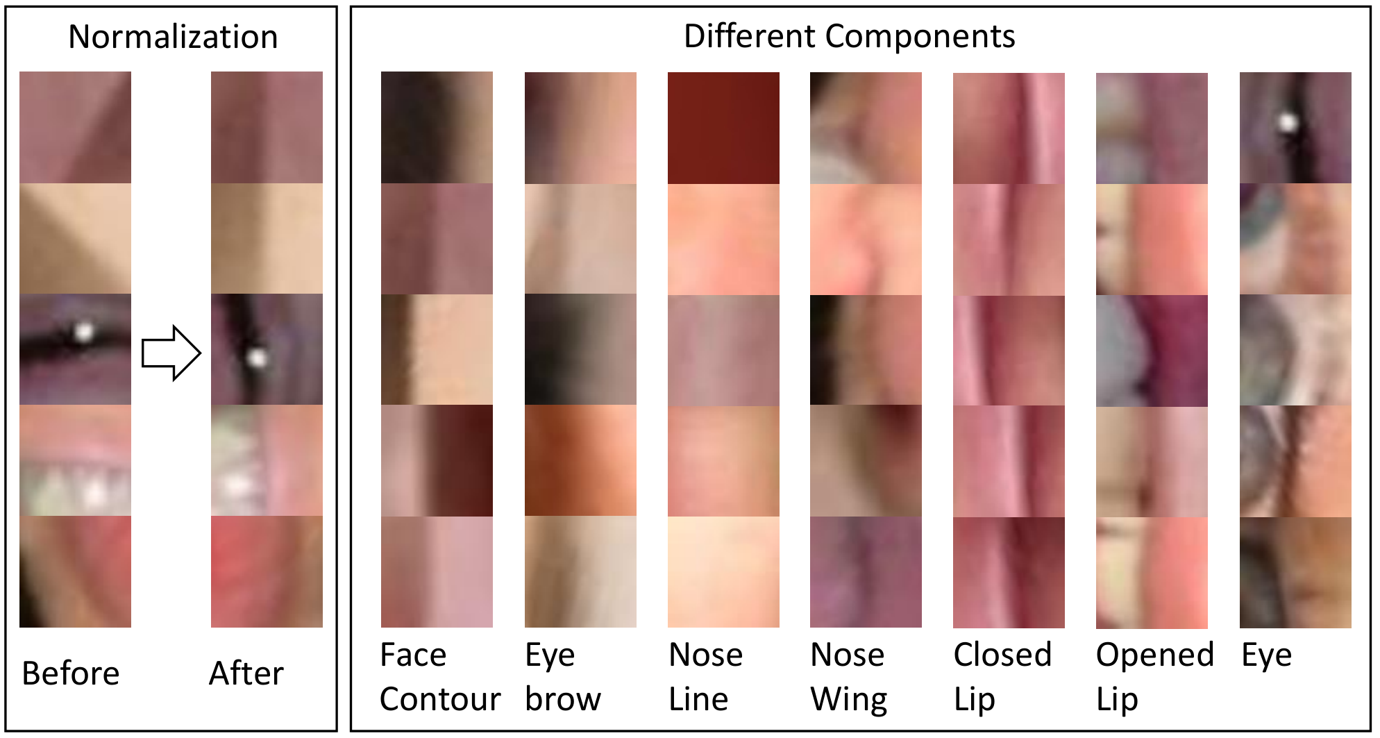
Patch Normalizing rotates each patch so that its -axis (horizontal direction) is aligned with the normal of the corresponding landmark along the contour line, which is illustrated in the left 2 columns of Fig. 3. The operator is based on the assumption that the precision improvement along the normal direction is more effective and reasonable than the tangent direction (Huang et al. 2021). Furthermore, the freedom of the regression target is reduced from 2D to 1D for no ambiguity and better convergence.
Quality Scoring is designed to handle blurry boundaries, occluded regions, and contour corners. The goal of this operator is to provide the reliability of each patch, which is used to weight the losses in training and provide confidence in testing. The intermediate value of the score is derived by
| (3) |
where and are the width and height of the local image patch, is the gray value of the specific pixel in th patch and is the standard deviation. Equation 3 is maximized when the variance along the horizontal direction is high, and the variance along the vertical direction is low, which aims to find a clear vertical boundary in the aligned image patch, in other words, those patches are suitable to regress the accurate rectification of the landmark because of the similar appearance and clear edge feature. The raw score of the patch is then obtained by
| (4) |
To normalize the raw score within 0 and 1, we firstly build a cumulative distribution function (CDF) using the whole patch scores in the training set, then map each raw score to the final normalized score by the cumulated probability in Equation 5.
| (5) |
where is the total number of patches in the training dataset. The distribution of the quality scores and their patch samples are shown in Fig. 4, which verifies the rationality in visual. In general, the aligned patch with a high-quality score has a clear vertical boundary, with a medium-quality score has a blurry boundary or occlusion, and with a low-quality score has a contour corner.

Index Embedding provides the position code of each patch similarity to transformer network (Vaswani et al. 2017). Specifically, we assign a soft index (position) to each patch (word) on the face (sentence).The right 7 columns of Fig. 3 show that the patches in the same component are similar, but there still exists a marginal appearance gap across components. Meanwhile, we can not put the patches of each landmark to the model in order, because of the misaligned landmark density between training and testing. For the above reasons, the index embedding in our framework is necessary to further improve the generalization of the model.
Assuming that the feature maps from the previous CNN layer have channels, then indices are selected as to filter channels from input feature maps, where is the number of anchor points. Given the soft index , the output feature maps of index embedding are presented as
| (6) |
To bridge the different landmark density between the training and testing stages of FreeEnricher, the soft index of could be calculated by
| (7) |
where is the enriched landmark. Specifically, is the anchor point, when , otherwise, the interpolated point.
Landmark Refining refines the initialized enriched landmarks by adding the regressed offset with normalized quality score as confidence (weight), which denotes as
| (8) |
where is the final refined enriched landmarks by FreeEnricher in inference.
Training process of FreeEnricher is presented in the upper part of Fig. 2, by inputting the face image and original landmarks , we firstly apply the offset generating to the original landmarks to generate the ground truth of offsets , which would distort the original landmarks , then feed the face image with distorted original landmarks to model (start from patch cropping and end in soft argmax) to get the regressed offsets and normalized quality scores , finally put them (, , ) to the loss function of FreeEnricher , which is defined as
| (9) |
where is the batch size, is the regressed offset, is the generated offset, and is the normalized quality score.
Testing process of FreeEnricher is demonstrated in the lower part of Fig. 2, by inputting the face image and original landmarks , we firstly employ the landmark initializing on the original landmarks to generate initialized enriched landmarks , then feed the face image with initialized enriched landmarks to model (start from patch cropping and end in soft argmax) to get the regressed offsets and normalized quality scores , finally put them (, , ) to landmark refining to acquire the final accurate enriched landmarks .
FreeEnricher Network
The model from FreeEnricher framework has the ability to enrich sparse landmarks to accurate dense landmarks. To make full use of this ability, we apply the FreeEnricher model to the existing face alignment networks (baseline networks) by plug-and-play mode, then get the FreeEnricher networks (enhanced networks). Specifically, there are two ways to plug in the model: (1) employing the model to pre-process the training dataset, which means densifying the ground truth of sparse landmarks, and (2) utilizing the model to postprocess the testing results, which denotes densifying the predicted value of sparse landmarks. Each way can be used optionally, thus we define the following 3 modes.
Plug in Test denotes that FreeEnricher only enriches the predicted landmarks in the testing stage. Under this mode, the total inference time increases tremendously.
Plug in Train indicates that FreeEnricher merely enriches the ground truth of landmarks in the training stage. Under this mode, there is no extra computational cost in inference, and it is the default mode in our method.
Plug in Train and Test means that FreeEnricher model enriches the ground truth of landmarks in the training stage with landmark initializing and refines the predicted landmarks in the testing stage without landmark initializing. Under this mode, the network always gets the highest accuracy, but it is pretty time-consuming in practical deployment.
| FreeEnricher Network | Baseline Network | Enriching Density | Plug in Train | Plug in Test |
| ResNet50-FE2train | ResNet50 | 2 | ✓ | ✗ |
| HRNet-FE3test | HRNet | 3 | ✗ | ✓ |
| ADNet-FE5 | ADNet | 5 | ✓ | ✗ |
| ADNet-FE10train+test | ADNet | 10 | ✓ | ✓ |
The name of FreeEnricher network is defined as ”-FE” in a unified format, where indicates which face alignment baseline network to be used, denotes the enriching density of landmark initializing and means in which stage the FreeEnricher plug, could be omitted when its value is ”train”. Several FreeEnricher network samples are presented in Table 1 for clearer understanding.
Experiment
Implementation Details
FreeEnricher. The FreeEnricher model is trained on four GPUs (16GB NVIDIA Tesla P100) by PyTorch (Paszke et al. 2019), where the batch size of each GPU is 68 for 300W and 98 for WFLW. We employ Adam optimizer with the initial learning rate of and decay the learning rate by at the epochs of 100, 150, and 180, finally ending at 200. Specifically, landmark initializing adopts b-spline interpolation method implemented in Scipy (Virtanen et al. 2020) with order of 3 and enriching density of 5, offset generating randomly generates offset by the uniform distribution , and patch cropping crops patch from aligned face image with resolution (patch-face ratio of 1/16) by the center of target landmark. The normalized patches are augmented by simulated random gray, random blur, and random occlusion. Regarding the backbone architecture of FreeEnricher, we adopt 3-stacked index embedding modules and 4-stacked hourglass modules, where each hourglass outputs a feature map. The output feature maps are then fed to (Huang et al. 2021) to generate the landmark offsets. The final landmark offset is from the last hourglass. The following experiments employ the settings above if no further explanation.
Face Alignment Network. The FreeEnricher model enhances the existing face alignment network by ”Plug in Train” mode in both landmark density and accuracy. And all of the existing face alignment networks are trained using the identical setting to the original papers.
Enriched 300W test set. We newly construct an enriched 300W test dataset by manually labeling the original images, which is employed to evaluate the performance of enriched face alignment. To handle different densities of landmarks, we labeled the continuous curve rather than discrete points. From the curve, firstly, we extract the anchor points by finding the points (on the curve) which are closest to the original landmark labels in 300W. Then, between two neighboring anchor points, the new points are uniformly sampled. For instance, from the original 68 landmarks, 320 enriched landmarks are generated with the enriching density 5. Typical samples are shown in Fig. 5.

Evaluation Metrics
Mean Error (ME) measures the averaged distance between predicted points and ground-truth points, which is specifically employed to evaluate the offset regression of fixed-scale patch in FreeEnricher model and defined as
| (10) |
where and , respectively, denotes the predicted values and the ground-truth of landmarks (or offsets), and is the number of landmarks (or offsets).
Normalized Mean Error of Points (NMEpoint or NME) between predicted points and ground-truth points is a widely-used standard metric to evaluate landmark accuracy for face alignment, which is defined as
| (11) |
where is the unit distance used to normalize the errors. Inter-ocular distance (distance between outer eye corners) is employed as the unit distance in the following experiments.
Normalized Mean Error of Edges (NMEedge) between predicted points and ground-truth edges is proposed to evaluate the performance of the landmarks, which emphasizes the error on the normal direction and is defined as
| (12) | ||||
where is the ground-truth of edges, is the edge that the th landmark belongs to, and computes point-to-edge distance.
Comparison on Enriched Landmarks
The main advantage of applying the FreeEnricher is that we get denser landmarks than from the original dataset. In order to demonstrate the effectiveness of FreeEnricher on enriching landmarks, we evaluate the NME of landmarks in the newly-constructed enriched 300W testing dataset. Because there is no existing method that could freely enrich landmarks, we design a baseline method as the comparison by applying landmark initializing operator, which enriches the landmark density of the original network. Meanwhile, the state-of-the-art ADNet is selected as the baseline network to be enhanced for a good starting point. Besides, other settings are identical between these 2 experiments. The result could be referred to Table 2, where FreeEnricher significantly enhances the accuracy of enriched landmarks, especially 20% improvement in the normal direction.
| Method | Network | NMEpoint | NMEedge |
| Baseline | ADNet + Line5 | 3.21 | 1.18 |
| Ours | ADNet-FE5 | 3.06 | 0.98 |
Comparison on Original Landmarks
Beyond enriching landmarks, the FreeEnricher can benefit the baseline network on the sparse landmarks as well. For the same reason, we still use ADNet as the baseline. Hence, we also evaluate FreeEnricher and the other face alignment algorithms on the original 300W and WFLW datasets in Table 3. The results show that FreeEnricher unexpectedly improves the accuracy further, and outperforms the existing methods on both 300W and WFLW.
| Method | 300W | WFLW |
| LAB (Wu et al. 2018) | 3.49 | 5.27 |
| HRNet (Wang et al. 2020) | 3.34 | 4.60 |
| LUVLi (Kumar et al. 2020) | 3.23 | 4.37 |
| ADNet (Huang et al. 2021) | 2.93 | 4.14 |
| ADNet-FE5 (Ours) | 2.87 | 4.10 |
Ablation Study
To verify the efficacy of FreeEnricher in unit and the contribution of each operator, we conduct comprehensive ablation experiments. Furthermore, they also demonstrate the robustness of different face alignment networks and the applicability to various landmark densities.
Unit Verification. To evaluate the offset refinement network independently from the whole system on local image patches, we conduct unit verification in Table 4. Hereon, FreeEnricher is trained on the generated patches from the training set and tested from the testing set respectively. Both the results on 300W and WFLW datasets demonstrate that FreeEnricher could refine the landmark location in the local patch of the face image.
| Method | 300W Testset | WFLW Testset |
| Random offset | 4.03 | 3.96 |
| Regressed offset | 1.92 | 1.89 |
Contribution of Each Operator. After integrating the designed operators into the framework individually, the performance increases to different degrees, which demonstrates the contribution of each operator in FreeEnricher framework. B-spline landmark initializing and patch normalizing improve more significantly than quality scoring and index embedding on accuracy. The best configuration is G in Table 5.
| Config. | Landmark Initializing | Patch Normalizing | Quality Scoring | Index Embedding | NME |
| A | - | - | - | - | 3.21 |
| B | line | ✗ | ✗ | ✗ | 3.18 |
| C | b-spline | ✗ | ✗ | ✗ | 3.11 |
| D | line | ✓ | ✗ | ✗ | 3.14 |
| E | line | ✗ | ✗ | ✓ | 3.16 |
| F | line | ✓ | ✓ | ✗ | 3.11 |
| G | b-spline | ✓ | ✓ | ✓ | 3.06 |
Robustness on Existing Network. The FreeEnricher could be plug-and-play to any face alignment network in theory. To verify the robustness in practice, several networks, ResNet50 (Zhang et al. 2014b), HRNet (Wang et al. 2020), and ADNet (Huang et al. 2021), are selected to conduct the comparison experiments. Table 6 demonstrate that all of them have a significant improvement on enriched 300W testing set after applying the FreeEnricher.
| Network | NME |
| ResNet50 + Line5 (Zhang et al. 2014b) | 4.76 |
| ResNet50-FE5 (Ours) | 4.39 |
| HRNet + Line5 (Wang et al. 2020) | 3.74 |
| HRNet-FE5 (Ours) | 3.46 |
| ADNet + Line5 (Huang et al. 2021) | 3.21 |
| ADNet-FE5 (Ours) | 3.06 |
Applicability on Enriching Density The FreeEnricher could enrich landmarks to arbitrary density in theory. To verify the applicability in practice, various enriching densities, 1, 2, 3, 5, and 10, are selected to conduct the verification experiments. Table 7 demonstrates that all of them achieve consistently high accuracy on the enriched 300W testing dataset by the given enriching density. Besides, the denser the landmarks are, the larger the NME becomes.
| Enriching Density | Landmarks Count | NME |
| 1 | 68 | 2.91 |
| 2 | 131 | 3.01 |
| 3 | 194 | 3.03 |
| 5 | 320 | 3.06 |
| 10 | 635 | 3.14 |
Study on Plugging Stage. The FreeEnricher could be plug-and-play in existing networks under their training and testing stage. The experiments in Table 8 illustrate that the FreeEnricher plugged in different stages have similar accuracy improvement but different computational cost in inference. To balance both high accuracy and low computational cost in the deployment environment, FreeEnricher is merely plugged in training stage. Then, FreeEnricher brings improvement on enriched landmarks without extra inference time and memory.
| Network | NME | Extra FLOPs | Extra Params |
| ADNet-FE5test | 3.07 | +9.85 G | +6.78 M |
| ADNet-FE5train | 3.06 | +0 G | +0 M |
| ADNet-FE5train+test | 3.04 | +9.85 G | +6.78 M |
Conclusion
Enriching facial landmarks is a meaningful topic in both academic and industry. In this paper, we present a novel idea to address this problem by using the existing datasets without additional labeling annotation and inference time costs. Moreover, our method could enrich landmarks to arbitrary density and be plug-and-play to any existing face alignment network in theory, which is also demonstrated by various experiments. Specifically, a weakly-supervised framework is proposed, which learns the refinement ability on original sparse landmarks of existing datasets, then this ability is applied to the initialized dense landmarks. By our method, we not only obtain accurate enriched facial landmarks but also achieve state-of-the-art performance in the original dataset.
References
- Browatzki and Wallraven (2020) Browatzki, B.; and Wallraven, C. 2020. 3fabrec: Fast few-shot face alignment by reconstruction. In Proceedings of the IEEE/CVF Conference on Computer Vision and Pattern Recognition, 6110–6120.
- Bulat and Tzimiropoulos (2016) Bulat, A.; and Tzimiropoulos, G. 2016. Convolutional aggregation of local evidence for large pose face alignment.
- Burgos-Artizzu, Perona, and Dollár (2013) Burgos-Artizzu, X. P.; Perona, P.; and Dollár, P. 2013. Robust face landmark estimation under occlusion. In Proceedings of the IEEE international conference on computer vision, 1513–1520.
- Cootes, Edwards, and Taylor (2001) Cootes, T. F.; Edwards, G. J.; and Taylor, C. J. 2001. Active appearance models. IEEE Transactions on pattern analysis and machine intelligence, 23(6): 681–685.
- Cootes and Taylor (1992) Cootes, T. F.; and Taylor, C. J. 1992. Active shape models—‘smart snakes’. In BMVC92, 266–275. Springer.
- Cootes et al. (1995) Cootes, T. F.; Taylor, C. J.; Cooper, D. H.; and Graham, J. 1995. Active shape models-their training and application. Computer vision and image understanding, 61(1): 38–59.
- Deng et al. (2019) Deng, J.; Trigeorgis, G.; Zhou, Y.; and Zafeiriou, S. 2019. Joint multi-view face alignment in the wild. IEEE Transactions on Image Processing, 28(7): 3636–3648.
- Dong et al. (2018) Dong, X.; Yan, Y.; Ouyang, W.; and Yang, Y. 2018. Style aggregated network for facial landmark detection. In Proceedings of the IEEE Conference on Computer Vision and Pattern Recognition, 379–388.
- Feng et al. (2018) Feng, Z.-H.; Kittler, J.; Awais, M.; Huber, P.; and Wu, X.-J. 2018. Wing loss for robust facial landmark localisation with convolutional neural networks. In Proceedings of the IEEE Conference on Computer Vision and Pattern Recognition, 2235–2245.
- Girshick (2015) Girshick, R. 2015. Fast r-cnn. In Proceedings of the IEEE international conference on computer vision, 1440–1448.
- Gundavarapu et al. (2019) Gundavarapu, N. B.; Srivastava, D.; Mitra, R.; Sharma, A.; and Jain, A. 2019. Structured Aleatoric Uncertainty in Human Pose Estimation. In CVPR Workshops, volume 2, 2.
- Huang and Tamrakar (2020) Huang, J.; and Tamrakar, A. 2020. ACE-Net: Fine-Level Face Alignment through Anchors and Contours Estimation. arXiv preprint arXiv:2012.01461.
- Huang et al. (2020) Huang, X.; Deng, W.; Shen, H.; Zhang, X.; and Ye, J. 2020. PropagationNet: Propagate Points to Curve to Learn Structure Information. In Proceedings of the IEEE/CVF Conference on Computer Vision and Pattern Recognition, 7265–7274.
- Huang et al. (2021) Huang, Y.; Yang, H.; Li, C.; Kim, J.; and Wei, F. 2021. ADNet: Leveraging Error-Bias Towards Normal Direction in Face Alignment. In Proceedings of the IEEE/CVF International Conference on Computer Vision, 3080–3090.
- Jiang et al. (2005) Jiang, D.; Hu, Y.; Yan, S.; Zhang, L.; Zhang, H.; and Gao, W. 2005. Efficient 3D reconstruction for face recognition. Pattern Recognition, 38(6): 787–798.
- Knott (2000) Knott, G. D. 2000. Interpolating cubic splines, volume 18. Springer Science & Business Media.
- Koestinger et al. (2011) Koestinger, M.; Wohlhart, P.; Roth, P. M.; and Bischof, H. 2011. Annotated facial landmarks in the wild: A large-scale, real-world database for facial landmark localization. In 2011 IEEE international conference on computer vision workshops (ICCV workshops), 2144–2151. IEEE.
- Kumar et al. (2020) Kumar, A.; Marks, T. K.; Mou, W.; Wang, Y.; Jones, M.; Cherian, A.; Koike-Akino, T.; Liu, X.; and Feng, C. 2020. LUVLi Face Alignment: Estimating Landmarks’ Location, Uncertainty, and Visibility Likelihood. In Proceedings of the IEEE/CVF Conference on Computer Vision and Pattern Recognition, 8236–8246.
- Liu et al. (2016) Liu, F.; Zeng, D.; Zhao, Q.; and Liu, X. 2016. Joint face alignment and 3D face reconstruction. In European Conference on Computer Vision, 545–560. Springer.
- Liu et al. (2017) Liu, Y.; Jourabloo, A.; Ren, W.; and Liu, X. 2017. Dense face alignment. In IEEE International Conference on Computer Vision Workshops, 1619–1628.
- Luo, Wang, and Tang (2012) Luo, P.; Wang, X.; and Tang, X. 2012. Hierarchical face parsing via deep learning. In 2012 IEEE Conference on Computer Vision and Pattern Recognition, 2480–2487. IEEE.
- Lv et al. (2017) Lv, J.; Shao, X.; Xing, J.; Cheng, C.; and Zhou, X. 2017. A deep regression architecture with two-stage re-initialization for high performance facial landmark detection. In Proceedings of the IEEE conference on computer vision and pattern recognition, 3317–3326.
- Masi et al. (2018) Masi, I.; Wu, Y.; Hassner, T.; and Natarajan, P. 2018. Deep face recognition: A survey. In 2018 31st SIBGRAPI conference on graphics, patterns and images (SIBGRAPI), 471–478. IEEE.
- Matthews and Baker (2004) Matthews, I.; and Baker, S. 2004. Active appearance models revisited. International journal of computer vision, 60(2): 135–164.
- Milborrow and Nicolls (2008) Milborrow, S.; and Nicolls, F. 2008. Locating facial features with an extended active shape model. In European conference on computer vision, 504–513. Springer.
- Newell, Yang, and Deng (2016) Newell, A.; Yang, K.; and Deng, J. 2016. Stacked hourglass networks for human pose estimation. In European conference on computer vision, 483–499. Springer.
- Paszke et al. (2019) Paszke, A.; Gross, S.; Massa, F.; Lerer, A.; Bradbury, J.; Chanan, G.; Killeen, T.; Lin, Z.; Gimelshein, N.; Antiga, L.; et al. 2019. Pytorch: An imperative style, high-performance deep learning library. Advances in neural information processing systems, 32.
- Qian et al. (2019) Qian, S.; Sun, K.; Wu, W.; Qian, C.; and Jia, J. 2019. Aggregation via separation: Boosting facial landmark detector with semi-supervised style translation. In Proceedings of the IEEE/CVF International Conference on Computer Vision, 10153–10163.
- Robinson et al. (2019) Robinson, J. P.; Li, Y.; Zhang, N.; Fu, Y.; and Tulyakov, S. 2019. Laplace landmark localization. In Proceedings of the IEEE/CVF International Conference on Computer Vision, 10103–10112.
- Ronneberger, Fischer, and Brox (2015) Ronneberger, O.; Fischer, P.; and Brox, T. 2015. U-net: Convolutional networks for biomedical image segmentation. In International Conference on Medical image computing and computer-assisted intervention, 234–241. Springer.
- Sagonas et al. (2013) Sagonas, C.; Tzimiropoulos, G.; Zafeiriou, S.; and Pantic, M. 2013. 300 faces in-the-wild challenge: The first facial landmark localization challenge. In Proceedings of the IEEE International Conference on Computer Vision Workshops, 397–403.
- Saragih and Goecke (2007) Saragih, J.; and Goecke, R. 2007. A nonlinear discriminative approach to AAM fitting. In 2007 IEEE 11th International Conference on Computer Vision, 1–8. IEEE.
- Sun, Wang, and Tang (2013) Sun, Y.; Wang, X.; and Tang, X. 2013. Deep convolutional network cascade for facial point detection. In Proceedings of the IEEE conference on computer vision and pattern recognition, 3476–3483.
- Toshev and Szegedy (2014) Toshev, A.; and Szegedy, C. 2014. Deeppose: Human pose estimation via deep neural networks. In Proceedings of the IEEE conference on computer vision and pattern recognition, 1653–1660.
- Trigeorgis et al. (2016) Trigeorgis, G.; Snape, P.; Nicolaou, M. A.; Antonakos, E.; and Zafeiriou, S. 2016. Mnemonic descent method: A recurrent process applied for end-to-end face alignment. In Proceedings of the IEEE Conference on Computer Vision and Pattern Recognition, 4177–4187.
- Vaswani et al. (2017) Vaswani, A.; Shazeer, N.; Parmar, N.; Uszkoreit, J.; Jones, L.; Gomez, A. N.; Kaiser, Ł.; and Polosukhin, I. 2017. Attention is all you need. In Advances in neural information processing systems, 5998–6008.
- Virtanen et al. (2020) Virtanen, P.; Gommers, R.; Oliphant, T. E.; Haberland, M.; Reddy, T.; Cournapeau, D.; Burovski, E.; Peterson, P.; Weckesser, W.; Bright, J.; et al. 2020. SciPy 1.0: fundamental algorithms for scientific computing in Python. Nature methods, 17(3): 261–272.
- Wang et al. (2020) Wang, J.; Sun, K.; Cheng, T.; Jiang, B.; Deng, C.; Zhao, Y.; Liu, D.; Mu, Y.; Tan, M.; Wang, X.; et al. 2020. Deep high-resolution representation learning for visual recognition. IEEE transactions on pattern analysis and machine intelligence.
- Wang, Bo, and Fuxin (2019) Wang, X.; Bo, L.; and Fuxin, L. 2019. Adaptive wing loss for robust face alignment via heatmap regression. In Proceedings of the IEEE/CVF International Conference on Computer Vision, 6971–6981.
- Wei et al. (2016) Wei, S.-E.; Ramakrishna, V.; Kanade, T.; and Sheikh, Y. 2016. Convolutional pose machines. In Proceedings of the IEEE conference on Computer Vision and Pattern Recognition, 4724–4732.
- Wu et al. (2018) Wu, W.; Qian, C.; Yang, S.; Wang, Q.; Cai, Y.; and Zhou, Q. 2018. Look at boundary: A boundary-aware face alignment algorithm. In Proceedings of the IEEE conference on computer vision and pattern recognition, 2129–2138.
- Zhang et al. (2014a) Zhang, J.; Shan, S.; Kan, M.; and Chen, X. 2014a. Coarse-to-fine auto-encoder networks (cfan) for real-time face alignment. In European conference on computer vision, 1–16. Springer.
- Zhang et al. (2014b) Zhang, Z.; Luo, P.; Loy, C. C.; and Tang, X. 2014b. Facial landmark detection by deep multi-task learning. In European conference on computer vision, 94–108. Springer.
- Zhou et al. (2013) Zhou, E.; Fan, H.; Cao, Z.; Jiang, Y.; and Yin, Q. 2013. Extensive facial landmark localization with coarse-to-fine convolutional network cascade. In Proceedings of the IEEE international conference on computer vision workshops, 386–391.
- Zhu et al. (2016) Zhu, X.; Lei, Z.; Liu, X.; Shi, H.; and Li, S. Z. 2016. Face alignment across large poses: A 3d solution. In Proceedings of the IEEE conference on computer vision and pattern recognition, 146–155.
References
- Browatzki and Wallraven (2020) Browatzki, B.; and Wallraven, C. 2020. 3fabrec: Fast few-shot face alignment by reconstruction. In Proceedings of the IEEE/CVF Conference on Computer Vision and Pattern Recognition, 6110–6120.
- Bulat and Tzimiropoulos (2016) Bulat, A.; and Tzimiropoulos, G. 2016. Convolutional aggregation of local evidence for large pose face alignment.
- Burgos-Artizzu, Perona, and Dollár (2013) Burgos-Artizzu, X. P.; Perona, P.; and Dollár, P. 2013. Robust face landmark estimation under occlusion. In Proceedings of the IEEE international conference on computer vision, 1513–1520.
- Cootes, Edwards, and Taylor (2001) Cootes, T. F.; Edwards, G. J.; and Taylor, C. J. 2001. Active appearance models. IEEE Transactions on pattern analysis and machine intelligence, 23(6): 681–685.
- Cootes and Taylor (1992) Cootes, T. F.; and Taylor, C. J. 1992. Active shape models—‘smart snakes’. In BMVC92, 266–275. Springer.
- Cootes et al. (1995) Cootes, T. F.; Taylor, C. J.; Cooper, D. H.; and Graham, J. 1995. Active shape models-their training and application. Computer vision and image understanding, 61(1): 38–59.
- Deng et al. (2019) Deng, J.; Trigeorgis, G.; Zhou, Y.; and Zafeiriou, S. 2019. Joint multi-view face alignment in the wild. IEEE Transactions on Image Processing, 28(7): 3636–3648.
- Dong et al. (2018) Dong, X.; Yan, Y.; Ouyang, W.; and Yang, Y. 2018. Style aggregated network for facial landmark detection. In Proceedings of the IEEE Conference on Computer Vision and Pattern Recognition, 379–388.
- Feng et al. (2018) Feng, Z.-H.; Kittler, J.; Awais, M.; Huber, P.; and Wu, X.-J. 2018. Wing loss for robust facial landmark localisation with convolutional neural networks. In Proceedings of the IEEE Conference on Computer Vision and Pattern Recognition, 2235–2245.
- Girshick (2015) Girshick, R. 2015. Fast r-cnn. In Proceedings of the IEEE international conference on computer vision, 1440–1448.
- Gundavarapu et al. (2019) Gundavarapu, N. B.; Srivastava, D.; Mitra, R.; Sharma, A.; and Jain, A. 2019. Structured Aleatoric Uncertainty in Human Pose Estimation. In CVPR Workshops, volume 2, 2.
- Huang and Tamrakar (2020) Huang, J.; and Tamrakar, A. 2020. ACE-Net: Fine-Level Face Alignment through Anchors and Contours Estimation. arXiv preprint arXiv:2012.01461.
- Huang et al. (2020) Huang, X.; Deng, W.; Shen, H.; Zhang, X.; and Ye, J. 2020. PropagationNet: Propagate Points to Curve to Learn Structure Information. In Proceedings of the IEEE/CVF Conference on Computer Vision and Pattern Recognition, 7265–7274.
- Huang et al. (2021) Huang, Y.; Yang, H.; Li, C.; Kim, J.; and Wei, F. 2021. ADNet: Leveraging Error-Bias Towards Normal Direction in Face Alignment. In Proceedings of the IEEE/CVF International Conference on Computer Vision, 3080–3090.
- Jiang et al. (2005) Jiang, D.; Hu, Y.; Yan, S.; Zhang, L.; Zhang, H.; and Gao, W. 2005. Efficient 3D reconstruction for face recognition. Pattern Recognition, 38(6): 787–798.
- Knott (2000) Knott, G. D. 2000. Interpolating cubic splines, volume 18. Springer Science & Business Media.
- Koestinger et al. (2011) Koestinger, M.; Wohlhart, P.; Roth, P. M.; and Bischof, H. 2011. Annotated facial landmarks in the wild: A large-scale, real-world database for facial landmark localization. In 2011 IEEE international conference on computer vision workshops (ICCV workshops), 2144–2151. IEEE.
- Kumar et al. (2020) Kumar, A.; Marks, T. K.; Mou, W.; Wang, Y.; Jones, M.; Cherian, A.; Koike-Akino, T.; Liu, X.; and Feng, C. 2020. LUVLi Face Alignment: Estimating Landmarks’ Location, Uncertainty, and Visibility Likelihood. In Proceedings of the IEEE/CVF Conference on Computer Vision and Pattern Recognition, 8236–8246.
- Liu et al. (2016) Liu, F.; Zeng, D.; Zhao, Q.; and Liu, X. 2016. Joint face alignment and 3D face reconstruction. In European Conference on Computer Vision, 545–560. Springer.
- Liu et al. (2017) Liu, Y.; Jourabloo, A.; Ren, W.; and Liu, X. 2017. Dense face alignment. In IEEE International Conference on Computer Vision Workshops, 1619–1628.
- Luo, Wang, and Tang (2012) Luo, P.; Wang, X.; and Tang, X. 2012. Hierarchical face parsing via deep learning. In 2012 IEEE Conference on Computer Vision and Pattern Recognition, 2480–2487. IEEE.
- Lv et al. (2017) Lv, J.; Shao, X.; Xing, J.; Cheng, C.; and Zhou, X. 2017. A deep regression architecture with two-stage re-initialization for high performance facial landmark detection. In Proceedings of the IEEE conference on computer vision and pattern recognition, 3317–3326.
- Masi et al. (2018) Masi, I.; Wu, Y.; Hassner, T.; and Natarajan, P. 2018. Deep face recognition: A survey. In 2018 31st SIBGRAPI conference on graphics, patterns and images (SIBGRAPI), 471–478. IEEE.
- Matthews and Baker (2004) Matthews, I.; and Baker, S. 2004. Active appearance models revisited. International journal of computer vision, 60(2): 135–164.
- Milborrow and Nicolls (2008) Milborrow, S.; and Nicolls, F. 2008. Locating facial features with an extended active shape model. In European conference on computer vision, 504–513. Springer.
- Newell, Yang, and Deng (2016) Newell, A.; Yang, K.; and Deng, J. 2016. Stacked hourglass networks for human pose estimation. In European conference on computer vision, 483–499. Springer.
- Paszke et al. (2019) Paszke, A.; Gross, S.; Massa, F.; Lerer, A.; Bradbury, J.; Chanan, G.; Killeen, T.; Lin, Z.; Gimelshein, N.; Antiga, L.; et al. 2019. Pytorch: An imperative style, high-performance deep learning library. Advances in neural information processing systems, 32.
- Qian et al. (2019) Qian, S.; Sun, K.; Wu, W.; Qian, C.; and Jia, J. 2019. Aggregation via separation: Boosting facial landmark detector with semi-supervised style translation. In Proceedings of the IEEE/CVF International Conference on Computer Vision, 10153–10163.
- Robinson et al. (2019) Robinson, J. P.; Li, Y.; Zhang, N.; Fu, Y.; and Tulyakov, S. 2019. Laplace landmark localization. In Proceedings of the IEEE/CVF International Conference on Computer Vision, 10103–10112.
- Ronneberger, Fischer, and Brox (2015) Ronneberger, O.; Fischer, P.; and Brox, T. 2015. U-net: Convolutional networks for biomedical image segmentation. In International Conference on Medical image computing and computer-assisted intervention, 234–241. Springer.
- Sagonas et al. (2013) Sagonas, C.; Tzimiropoulos, G.; Zafeiriou, S.; and Pantic, M. 2013. 300 faces in-the-wild challenge: The first facial landmark localization challenge. In Proceedings of the IEEE International Conference on Computer Vision Workshops, 397–403.
- Saragih and Goecke (2007) Saragih, J.; and Goecke, R. 2007. A nonlinear discriminative approach to AAM fitting. In 2007 IEEE 11th International Conference on Computer Vision, 1–8. IEEE.
- Sun, Wang, and Tang (2013) Sun, Y.; Wang, X.; and Tang, X. 2013. Deep convolutional network cascade for facial point detection. In Proceedings of the IEEE conference on computer vision and pattern recognition, 3476–3483.
- Toshev and Szegedy (2014) Toshev, A.; and Szegedy, C. 2014. Deeppose: Human pose estimation via deep neural networks. In Proceedings of the IEEE conference on computer vision and pattern recognition, 1653–1660.
- Trigeorgis et al. (2016) Trigeorgis, G.; Snape, P.; Nicolaou, M. A.; Antonakos, E.; and Zafeiriou, S. 2016. Mnemonic descent method: A recurrent process applied for end-to-end face alignment. In Proceedings of the IEEE Conference on Computer Vision and Pattern Recognition, 4177–4187.
- Vaswani et al. (2017) Vaswani, A.; Shazeer, N.; Parmar, N.; Uszkoreit, J.; Jones, L.; Gomez, A. N.; Kaiser, Ł.; and Polosukhin, I. 2017. Attention is all you need. In Advances in neural information processing systems, 5998–6008.
- Virtanen et al. (2020) Virtanen, P.; Gommers, R.; Oliphant, T. E.; Haberland, M.; Reddy, T.; Cournapeau, D.; Burovski, E.; Peterson, P.; Weckesser, W.; Bright, J.; et al. 2020. SciPy 1.0: fundamental algorithms for scientific computing in Python. Nature methods, 17(3): 261–272.
- Wang et al. (2020) Wang, J.; Sun, K.; Cheng, T.; Jiang, B.; Deng, C.; Zhao, Y.; Liu, D.; Mu, Y.; Tan, M.; Wang, X.; et al. 2020. Deep high-resolution representation learning for visual recognition. IEEE transactions on pattern analysis and machine intelligence.
- Wang, Bo, and Fuxin (2019) Wang, X.; Bo, L.; and Fuxin, L. 2019. Adaptive wing loss for robust face alignment via heatmap regression. In Proceedings of the IEEE/CVF International Conference on Computer Vision, 6971–6981.
- Wei et al. (2016) Wei, S.-E.; Ramakrishna, V.; Kanade, T.; and Sheikh, Y. 2016. Convolutional pose machines. In Proceedings of the IEEE conference on Computer Vision and Pattern Recognition, 4724–4732.
- Wu et al. (2018) Wu, W.; Qian, C.; Yang, S.; Wang, Q.; Cai, Y.; and Zhou, Q. 2018. Look at boundary: A boundary-aware face alignment algorithm. In Proceedings of the IEEE conference on computer vision and pattern recognition, 2129–2138.
- Zhang et al. (2014a) Zhang, J.; Shan, S.; Kan, M.; and Chen, X. 2014a. Coarse-to-fine auto-encoder networks (cfan) for real-time face alignment. In European conference on computer vision, 1–16. Springer.
- Zhang et al. (2014b) Zhang, Z.; Luo, P.; Loy, C. C.; and Tang, X. 2014b. Facial landmark detection by deep multi-task learning. In European conference on computer vision, 94–108. Springer.
- Zhou et al. (2013) Zhou, E.; Fan, H.; Cao, Z.; Jiang, Y.; and Yin, Q. 2013. Extensive facial landmark localization with coarse-to-fine convolutional network cascade. In Proceedings of the IEEE international conference on computer vision workshops, 386–391.
- Zhu et al. (2016) Zhu, X.; Lei, Z.; Liu, X.; Shi, H.; and Li, S. Z. 2016. Face alignment across large poses: A 3d solution. In Proceedings of the IEEE conference on computer vision and pattern recognition, 146–155.
Appendix A Appendix
In order to introduce the paper more clearly and provide more information as a reference, we add supplementary material as an appendix. Briefly speaking, the supplementary material contains three sections, firstly, the application of facial morphometric measurement demonstrates the significance of enriching landmarks in downstream tasks, then, the additional details of the proposed approach are also provided including landmark contour definition, landmark contour fitting, landmark normal calculation, and regression model architecture, finally, in order to further verify the efficacy of our method on different facial components and different extreme scenarios, several additional experiments are conducted, and the visualization result on 300W and WflW test sets furtherly proves it.
Appendix B Application
Facial Morphometric Measures
Facial morphometric measures are widely used in cosmetic medicine to help with disease diagnosis and aesthetic analysis. While the measures are usually calculated from landmarks, especially dense landmarks.To illustrate the significance of enriching landmarks on downstream tasks, several facial morphometric measures, chin angle, jaw area, and the ratio of the upper and lower lip area, are designed based on existing facial landmarks in Fig 6. These facial morphometric measures are intuitive and discriminative on the face images of the 300W dataset.


By the MAPE in Table 9, the predicted enriched landmarks outperform sparse landmarks even in ground-truth landmarks, when applying them to the facial morphometric measures. To conclude, dense landmarks are better than sparse landmarks in the application of facial morphometric measures. Enriching landmarks is meaningful for some downstream tasks.


| Method | Landmarks | Chin Angle | LeftJaw Area | RightJaw Area | LipArea Ratio |
| ADNet (Huang et al. 2021) | Sparse | 1.414 | 5.950 | 6.223 | 5.146 |
| Ground-truth | Sparse | 1.317 | 5.355 | 5.483 | 5.514 |
| ADNet-FE5 (Ours) | dense | 0.369 | 3.189 | 3.091 | 4.373 |
Appendix C Additional Details
Landmark Contour Definition
We divide the facial landmark points into several landmark contours according to their semantic relations, they are facial contour, left/right eyebrow, left/right eye, nose middle/bottom line, inner/outer lip, and left/right pupil. For the 300W and WFLW datasets, there are 9 and 11 landmark groups, respectively, as shown in Table 10 and Fig. 8. Except for the two isolated landmarks of pupils in WFLW, all the landmarks are located on an edge or a contour line.
| Facial Component Names | 300W | WFLW | ||
| Original Indices | Enriched Indices | Original Indices | Enriched Indices | |
| Facial Contour | 0-16 | 0-80 | 0-32 | 0-160 |
| Eyebrow Right | 17-21 | 81-101 | 33-41 | 161-205 |
| Eyebrow Left | 22-26 | 102-122 | 42-50 | 206-250 |
| Nose Middle Line | 27-30 | 123-138 | 51-54 | 251-266 |
| Nose Bottom Line | 31-35 | 139-159 | 55-59 | 267-287 |
| Eye Right | 36-41 | 160-189 | 60-67 | 288-327 |
| Eye Left | 42-47 | 190-219 | 68-75 | 328-367 |
| Lip Outer | 48-59 | 220-279 | 76-87 | 368-427 |
| Lip Inner | 60-67 | 280-319 | 88-95 | 428-467 |
| Pupil Right | - | - | 96 | 468 |
| Pupil Left | - | - | 97 | 469 |
| Whole Face | 0-67 | 0-319 | 0-97 | 0-469 |

Landmark Contour Fitting
To initialize the enriched facial landmarks, both straight line and b-spline (Knott 2000) could be adopted to roughly fit the facial contour in Fig. 9. For instance of b-spline, it is a general form of bezier curve, which is a linear combination of control points and basic functions. B-spline has continuous derivatives in each split point but each segment has an independent shape. Given a set of ordered points, b-spline can be fitted as
| (13) |
where is the control point, is the order, is the number of knots, is the basis function, and is the input variable to control the position of a point in curve. For the given sparse landmarks belonging to one edge, each of them could be used as a knot to fit the curve. Thus, b-spline is applied to each independent facial component having contour or line information, such as eye, mouth and face contour.

| Facial Component Names | Facial Contour | Eyebrow Right | Eyebrow Left | Nose Middle Line | Nose Bottom Line | Eye Right | Eye Left | Lip Outer | Lip Inner | Whole Face | |
| Avg. | 7.719 | 4.009 | 3.931 | 1.267 | 1.267 | 2.968 | 2.061 | 3.013 | 3.139 | 3.964 | |
| NMEpoint | ADNet+Line5 | 5.617 | 3.240 | 3.125 | 1.990 | 2.538 | 1.639 | 1.601 | 2.080 | 4.014 | 3.208 |
| ADNet-FE5 | 5.282 | 2.984 | 2.848 | 1.888 | 2.618 | 1.490 | 1.472 | 1.889 | 3.711 | 3.061 | |
| NMEedge | ADNet+Line5 | 1.541 | 1.136 | 1.134 | 0.880 | 1.270 | 0.934 | 0.932 | 0.988 | 0.973 | 1.183 |
| ADNet-FE5 | 1.374 | 1.058 | 1.060 | 0.873 | 1.208 | 0.666 | 0.636 | 0.827 | 0.757 | 0.976 | |
| Method | Testset | Pose Subset | Expression Subset | Illumination Subset | Make-up Subset | Occlusion Subset | Blur Subset |
| LAB (Wu et al. 2018) | 5.27 | 10.24 | 5.51 | 5.23 | 5.15 | 6.79 | 6.12 |
| HRNet (Wang et al. 2020) | 4.60 | 7.86 | 4.78 | 4.57 | 4.26 | 5.42 | 5.36 |
| ADNet (Huang et al. 2021) | 4.14 | 6.96 | 4.38 | 4.09 | 4.05 | 5.06 | 4.79 |
| ADNet-FE5 (Ours) | 4.10 | 6.94 | 4.38 | 4.07 | 3.91 | 4.92 | 4.71 |
Landmark Normal Calculation
Based on the fitted curve, denoted by , the derivative of the curve can be calculated by following (prochazkova2005derivative). Hereon, is also a b-spline curve with the order of on the original knot vector and the new set of control points. Then the normal direction of the enriched landmarks in the fitted b-spline could be derived by using , which is a necessary dependence for the patch normalizing operator in FreeEnricher.
Regression Model Architecture
Fig. 10 demonstrates the detailed architecture of the offset regression model. Except for the layer that is devised in this paper, the other layers are all widely-used layers. In the case of and , there are 4 hyperparameters which consist of the number of input channels, the number of output channels, the kernel size, and the stride respectively. layer, module, (Batch normalization) layer and layer have 2 hyperparameters which are the number of input and output channels.
Appendix D Additional Experiments
Evaluation on Different Components
Apart from evaluating the performance of the whole facial landmarks, we also provide the individual results on different facial components defined in Table 10. As we only have the ground truth for the enriched 300W testing set, the experiments are conducted on it as tabulated in Table 11. Compared with baseline ADNet, there are two important observations. First, FreeEnricher has more improvement on NMEedge(20%) than on NMEpoint(5%), which indicates that the improvement along the normal direction is more significant. Second, FreeEnricher results in great accuracy improvement on facial components having obvious edge features, such as facial contours and eyes.
Evaluation on Extreme Scenarios
To verify the effectiveness of our method in extreme scenarios, we conduct experiments on subset of WFLW testset. For the reason, would assign a low weight to the extreme cases, and would adjust their location carefully by the weight, the performance of those points are stable or even better, which is demonstrated in Table 12.
Comparison of Visualized Results
To show the extended qualitative results, we randomly select samples in 300W testing dataset in Fig. 11. We observe that ADNet-FE5 infers landmarks more tightly to the corresponding contours than the baseline method, and there is no regression in the occluded or blurry regions. Several samples on WFLW are also illustrated in Fig. 12, where only the inference results of ADNet-FE5 are shown since there is no ground truth of the enriched landmark. It is recommended to zoom in the images for better discrimination.

