跳到论文正文
W Papers独立论文阅读器 arXiv:2212.09494 论文正文 计算阅读时间 · 0%
引用这篇论文根据当前论文元数据生成,正式投稿前建议核对。


License: arXiv.org perpetual non-exclusive license
arXiv:2212.09494v3 [stat.ME] 24 Oct 2023

Optimal Treatment Regimes for Proximal
Causal LearningThanks: Correspondence to Yifan Cui <<cuiyf@zju.edu.cn>>

Tao Shen Affiliation: National University of Singapore Affiliation: Yifan Cui Affiliation: Zhejiang University
Abstract

A common concern when a policymaker draws causal inferences from and makes decisions based on observational data is that the measured covariates are insufficiently rich to account for all sources of confounding, i.e., the standard no confoundedness assumption fails to hold. The recently proposed proximal causal inference framework shows that proxy variables that abound in real-life scenarios can be leveraged to identify causal effects and therefore facilitate decision-making. Building upon this line of work, we propose a novel optimal individualized treatment regime based on so-called outcome and treatment confounding bridges. We then show that the value function of this new optimal treatment regime is superior to that of existing ones in the literature. Theoretical guarantees, including identification, superiority, excess value bound, and consistency of the estimated regime, are established. Furthermore, we demonstrate the proposed optimal regime via numerical experiments and a real data application.

1 Introduction

Data-driven individualized decision-making has received tremendous attention nowadays due to its applications in healthcare, economics, marketing, etc. A large branch of work has focused on maximizing the expected utility of implementing the estimated optimal policy over a target population based on randomized controlled trials or observational studies, e.g., Athey and Wager 2021; Chakraborty and Moodie 2013; Jiang et al. 2019; Kitagawa and Tetenov 2018; Kosorok and Laber 2019; Murphy 2003; Qian and Murphy 2011; Robins 1986; Robins 1994; Robins 1997; Tsiatis et al. 2019; Wu et al. 2019; Zhao et al. 2012; Zhao et al. 2019.

A critical assumption commonly made in these studies, known as unconfoundedness or exchangeability, precludes the existence of unmeasured confounding. Relying on an assumed ability of the decision-maker to accurately measure covariates relevant to a variety of confounding mechanisms present in a given observational study, causal effects, value functions, and other relevant quantities can be nonparametrically identified. However, such an assumption might not always be realistic in observational studies or randomized trials subject to non-compliance (Robins 1994; Robins 1997). Therefore, it is of great interest in recovering confounding mechanisms from measured covariates to infer causal effects and facilitate decision-making. A prevailing strand of work has been devoted to using instrumental variable (Angrist et al. 1996; Imbens and Angrist 1994) as a proxy variable in dynamic treatment regimes and reinforcement learning settings (Cui 2021; Cui and Tchetgen Tchetgen 2021b; Cui and Tchetgen Tchetgen 2021a; Han 2023; Liao et al. 2021; Pu and Zhang 2021; Qiu et al. 2021; Stensrud and Sarvet 2022).

Recently, Tchetgen Tchetgen et al. proposed the so-called proximal causal inference framework, a formal potential outcome framework for proximal causal learning, which while explicitly acknowledging covariate measurements as imperfect proxies of confounding mechanisms, establishes causal identification in settings where exchangeability on the basis of measured covariates fails. Rather than as current practice dictates, assuming that adjusting for all measured covariates, unconfoundedness can be attained, proximal causal inference essentially requires that the investigator can correctly classify a subset of measured covariates L∈ℒL\in\mathcal{L} into three types: i) variables X∈𝒳X\in\mathcal{X} that may be common causes of the treatment and outcome variables; ii) treatment-inducing confounding proxies Z∈𝒵Z\in\mathcal{Z}; and iii) outcome-inducing confounding proxies W∈𝒲W\in\mathcal{W}.

There is a fast-growing literature on proximal causal inference since it has been proposed (Cui et al. 2023; Dukes et al. 2023; Ghassami et al. 2023; Kompa et al. 2022; Li et al. 2023; Mastouri et al. 2021; Miao et al. 2018b; Shi et al. 2020b; Shi et al. 2021; Shpitser et al. 2023; Singh 2020; Tchetgen Tchetgen et al. 2020; Ying et al. 2023; Ying et al. 2022 and many others). In particular, Miao et al. 2018a; Tchetgen Tchetgen et al. 2020 propose identification of causal effects through an outcome confounding bridge and Cui et al. 2023 propose identification through a treatment confounding bridge. A doubly robust estimation strategy (Chernozhukov et al. 2018; Robins et al. 1994; Rotnitzky et al. 1998; Scharfstein et al. 1999) is further proposed in Cui et al. 2023. In addition, Ghassami et al. 2022 and Kallus et al. 2021 propose a nonparametric estimation of causal effects through a min-max approach. Moreover, by adopting the proximal causal inference framework, Qi et al. 2023 consider optimal individualized treatment regimes (ITRs) estimation, Sverdrup and Cui 2023 consider learning heterogeneous treatment effects, and Bennett and Kallus 2023 consider off-policy evaluation in partially observed Markov decision processes.

In this paper, we aim to estimate optimal ITRs under the framework of proximal causal inference. We start with reviewing two in-class ITRs that map from 𝒳×𝒲\mathcal{X}\times\mathcal{W} to 𝒜\mathcal{A} and 𝒳×𝒵\mathcal{X}\times\mathcal{Z} to 𝒜\mathcal{A}, respectively, where 𝒜\mathcal{A} denotes the binary treatment space. The identification of value function and the learning strategy for these two optimal in-class ITRs are proposed in Qi et al. 2023. In addition, Qi et al. 2023 also consider a maximum proximal learning optimal ITR that maps from 𝒳×𝒲×𝒵\mathcal{X}\times\mathcal{W}\times\mathcal{Z} to 𝒜\mathcal{A} with the ITRs being restricted to either 𝒳×𝒲→𝒜\mathcal{X}\times\mathcal{W}\rightarrow\mathcal{A} or 𝒳×𝒵→𝒜\mathcal{X}\times\mathcal{Z}\rightarrow\mathcal{A}. In contrast to their maximum proximal learning ITR, in this paper, we propose a brand new policy class whose ITRs map from measured covariates 𝒳×𝒲×𝒵\mathcal{X}\times\mathcal{W}\times\mathcal{Z} to 𝒜\mathcal{A}, which incorporates the predilection between these two in-class ITRs. Identification and superiority of the proposed optimal ITRs compared to existing ones are further established.

The main contributions of our work are four-fold. Firstly, by leveraging treatment and outcome confounding bridges under the recently proposed proximal causal inference framework, identification results regarding the proposed class 𝒟𝒵​𝒲Π\mathcal{D}_{\mathcal{ZW}}^{\Pi} of ITRs that map 𝒳×𝒲×𝒵\mathcal{X}\times\mathcal{W}\times\mathcal{Z} to 𝒜\mathcal{A} are established. The proposed ITR class can be viewed as a generalization of existing ITR classes proposed in the literature. Secondly, an optimal subclass of 𝒟𝒵​𝒲Π\mathcal{D}_{\mathcal{ZW}}^{\Pi} is further introduced. Learning optimal treatment regimes within this subclass leads to a superior value function. Thirdly, we propose a learning approach to estimating the proposed optimal ITR. Our learning pipeline begins with the estimation of confounding bridges adopting the deep neural network method proposed by Kompa et al. 2022. Then we use optimal treatment regimes proposed in Qi et al. 2023 as preliminary regimes to estimate our optimal ITR. Lastly, we establish an excess value bound for the value difference between the estimated treatment regime and existing ones in the literature, and the consistency of the estimated regime is also demonstrated.

2 Methodology

2.1 Optimal individualized treatment regimes

We briefly introduce some conventional notation for learning optimal ITRs. Suppose AA is a binary variable representing a treatment option that takes values in the treatment space 𝒜={−1,1}\mathcal{A}=\{-1,1\}. Let L∈ℒL\in\mathcal{L} be a vector of observed covariates, and YY be the outcome of interest. Let Y⁡(1)Y(1) and Y⁡(−1)Y(-1) be the potential outcomes under an intervention that sets the treatment to values 11 and −1-1, respectively. Without loss of generality, we assume that larger values of YY are preferred.

Suppose the following standard causal assumptions hold: (1) Consistency: Y=Y⁡(A)Y=Y(A). That is, the observed outcome matches the potential outcome under the realized treatment. (2) Positivity: ℙ⁡(A=a|L)>0\mathbb{P}(A=a|L)>0 for a∈𝒜a\in\mathcal{A} almost surely, i.e., both treatments are possible to be assigned.

We consider an ITR class 𝒟\mathcal{D} containing ITRs that are measurable functions mapping from the covariate space ℒ\mathcal{L} onto the treatment space 𝒜\mathcal{A}. For any d∈𝒟d\in\mathcal{D}, the potential outcome under a hypothetical intervention that assigns treatment according to dd is defined as

Y(d(L))=△Y(1)𝕀{d(L)=1}+Y(−1)𝕀{d(L)=−1},Y(d(L))\overset{\triangle}{=}Y(1)\mathbb{I}\{d(L)=1\}+Y(-1)\mathbb{I}\{d(L)=-1\},

where 𝕀​{⋅}\mathbb{I}\{\cdot\} denotes the indicator function. The value function of ITR dd is defined as the expectation of the potential outcome, i.e.,

V⁡(d)​=△​𝔼​[Y⁡(d⁡(L))].V(d)\overset{\triangle}{=}\mathbb{E}[Y(d(L))].

It can be easily seen that an optimal ITR can be expressed as

d∗​(L)=sign​{𝔼⁡(Y⁡(1)−Y⁡(−1)|L)}\displaystyle d^{*}(L)=\text{sign}\{\mathbb{E}(Y(1)-Y(-1)|L)\}

or

d∗=arg⁡maxd∈𝒟⁡𝔼⁡[Y⁡(d⁡(L))].\displaystyle d^{*}=\arg\max_{d\in\mathcal{D}}\mathbb{E}[Y(d(L))].

There are many ways to identify optimal ITRs under different sets of assumptions. The most commonly seen assumption is the unconfoundedness: Y⁡(a)⟂A|LY(a)\perp A|L for a=±1a=\pm 1, i.e., upon conditioning on LL, there is no unmeasured confounder affecting both AA and YY. Under this unconfoundedness assumption, the value function of a given regime dd can be identified by (Qian and Murphy 2011)

V⁡(d)=𝔼⁡[Y𝕀{A=d(L)}f⁡(A|L)],V(d)=\mathbb{E}\left[\frac{Y\mathbb{I}\{A=d(L)\}}{f(A|L)}\right],

where f⁡(A|L)f(A|L) denotes the propensity score (Rosenbaum and Rubin 1983), and the optimal ITR is identified by

d∗=arg⁡maxd∈𝒟⁡V⁡(d)=arg⁡maxd∈𝒟⁡𝔼⁡[Y𝕀{A=d(L)}f⁡(A|L)].d^{*}=\arg\max_{d\in\mathcal{D}}V(d)=\arg\max_{d\in\mathcal{D}}\mathbb{E}\left[\frac{Y\mathbb{I}\{A=d(L)\}}{f(A|L)}\right].

We refer to Qian and Murphy 2011; Zhang et al. 2012; Zhao et al. 2012 for more details of learning optimal ITRs in this unconfounded setting.

Because confounding by unmeasured factors cannot generally be ruled out with certainty in observational studies or randomized experiments subject to non-compliance, skepticism about the unconfoundedness assumption in observational studies is often warranted. To estimate optimal ITRs subject to potential unmeasured confounding, Cui and Tchetgen Tchetgen 2021b propose instrumental variable approaches to learning optimal ITRs. Under certain instrumental variable assumptions, the optimal ITR can be identified by

arg⁡maxd∈𝒟⁡𝔼⁡[MAY𝕀{A=d(L)}{ℙ⁡(A=1|M=1,L)−ℙ⁡(A=1|M=−1,L)}​f​(M|L)],\arg\max_{d\in\mathcal{D}}\mathbb{E}\left[\frac{MAY\mathbb{I}\{A=d(L)\}}{\{\mathbb{P}(A=1|M=1,L)-\mathbb{P}(A=1|M=-1,L)\}f(M|L)}\right],

where MM denotes a valid binary instrumental variable. Other works including Cui 2021; Cui and Tchetgen Tchetgen 2021a; Han 2023; Pu and Zhang 2021 consider a sign or partial identification of causal effects to estimate suboptimal ITRs using instrumental variables.

2.2 Existing optimal ITRs for proximal causal inference

Another line of research in causal inference considers negative control variables as proxies to mitigate confounding bias (Kuroki and Pearl 2014; Miao et al. 2018a; Shi et al. 2020a; Tchetgen Tchetgen 2014). Recently, a formal potential outcome framework, namely proximal causal inference, has been developed by Tchetgen Tchetgen et al. 2020, which has attracted tremendous attention since proposed.

Following the proximal causal inference framework proposed in Tchetgen Tchetgen et al. 2020, suppose that the measured covariate LL can be decomposed into three buckets L=(X,W,Z)L=(X,W,Z), where X∈𝒳X\in\mathcal{X} affects both AA and YY, W∈𝒲W\in\mathcal{W} denotes an outcome-inducing confounding proxy that is a potential cause of the outcome which is related with the treatment only through (U,X)(U,X), and Z∈𝒵Z\in\mathcal{Z} is a treatment-inducing confounding proxy that is a potential cause of the treatment which is related with the outcome YY through (U,X,A)(U,X,A). We now summarize several basic assumptions of the proximal causal inference framework.

Assumption 1.

We make the following assumptions:
(1) Consistency: Y=Y⁡(A,Z),W=W⁡(A,Z)Y=Y(A,Z),\ W=W(A,Z).
(2) Positivity: ℙ⁡(A=a|U,X)>0,∀a∈𝒜.\mathbb{P}(A=a\ |\ U,X)>0,\ \forall a\in\mathcal{A}.
(3) Latent unconfoundedness:
(Z,A)⟂(Y⁡(a),W)|U,X,∀a∈𝒜.(Z,A)\perp(Y(a),W)\ |\ U,X,\ \forall a\in\mathcal{A}.

The consistency and positivity assumptions are conventional in the causal inference literature. The latent unconfoundedness essentially states that ZZ cannot directly affect the outcome YY, and WW is not directly affected by either AA or ZZ. Figure 1 depicts a classical setting that satisfies Assumption 1. We refer to Shi et al. 2020b; Tchetgen Tchetgen et al. 2020 for other realistic settings for proximal causal inference.

XXZZWWUUAAYY
Figure 1: A causal DAG under the proximal causal inference framework.

We first consider two in-class optimal ITRs that map from 𝒳×𝒵\mathcal{X}\times\mathcal{Z} to 𝒜\mathcal{A} and 𝒳×𝒲\mathcal{X}\times\mathcal{W} to 𝒜\mathcal{A}, respectively. To identify optimal ITRs that map from 𝒳×𝒵\mathcal{X}\times\mathcal{Z} to 𝒜\mathcal{A}, we make the following assumptions.

Assumption 2.

Completeness: For any a∈𝒜,x∈𝒳a\in\mathcal{A},x\in\mathcal{X} and square-integrable function gg, 𝔼[g(U)|Z,A=a,X=x]=0\mathbb{E}[g(U)\ |\ Z,A=a,X=x]=0 almost surely if and only if g⁡(U)=0g(U)=0 almost surely.

Assumption 3.

Existence of outcome confounding bridge: There exists an outcome confounding bridge function h⁡(w,a,x)h(w,a,x) that solves the following equation

𝔼[Y|Z,A,X]=𝔼[h(W,A,X)|Z,A,X],\mathbb{E}[Y|Z,A,X]=\mathbb{E}[h(W,A,X)|Z,A,X],

almost surely.

The completeness Assumption 2 is a technical condition central to the study of sufficiency in foundational theory of statistical inference. It essentially assumes that ZZ has sufficient variability with respect to the variability of UU. We refer to Tchetgen Tchetgen et al. 2020 and Miao et al. 2022 for further discussions regarding the completeness condition. Assumption 3 defines a so-called inverse problem known as a Fredholm integral equation of the first kind through an outcome confounding bridge. The technical conditions for the existence of a solution to a Fredholm integral equation can be found in Kress et al. 1989.

Let 𝒟𝒵\mathcal{D}_{\mathcal{Z}} be an ITR class that includes all measurable functions mapping from 𝒳×𝒵\mathcal{X}\times\mathcal{Z} to 𝒜\mathcal{A}. As shown in Qi et al. 2023, under Assumptions 1, 2 and 3, for any dz∈𝒟𝒵d_{z}\in\mathcal{D}_{\mathcal{Z}}, the value function V⁡(dz)V(d_{z}) can be nonparametrically identified by

V⁡(dz)=𝔼⁡[h⁡(W,dz​(X,Z),X)].V(d_{z})=\mathbb{E}[h(W,d_{z}(X,Z),X)]. (1)

Furthermore, the in-class optimal treatment regime dz∗∈arg⁡maxdz∈𝒟𝒵⁡V⁡(dz)d_{z}^{*}\in\arg\max_{d_{z}\in\mathcal{D}_{\mathcal{Z}}}V(d_{z}) is given by

dz∗(X,Z)=sign{𝔼[h(W,1,X)−h(W,−1,X)|X,Z]}.d_{z}^{*}(X,Z)=\text{sign}\{\mathbb{E}[h(W,1,X)-h(W,-1,X)|X,Z]\}.

On the other hand, to identify optimal ITRs that map from 𝒳×𝒲\mathcal{X}\times\mathcal{W} to 𝒜\mathcal{A}, we make the following assumptions.

Assumption 4.

Completeness: For any a∈𝒜,x∈𝒳a\in\mathcal{A},x\in\mathcal{X} and square-integrable function gg, 𝔼[g(U)|W,A=a,X=x]=0\mathbb{E}[g(U)\ |\ W,A=a,X=x]=0 almost surely if and only if g⁡(U)=0g(U)=0 almost surely.

Assumption 5.

Existence of treatment confounding bridge: There exists a treatment confounding bridge function q⁡(z,a,x)q(z,a,x) that solves the following equation

1ℙ⁡(A=a|W,X)=𝔼[q(Z,a,X)|W,A=a,X],\frac{1}{\mathbb{P}(A=a|W,X)}=\mathbb{E}[q(Z,a,X)|W,A=a,X],

almost surely.

Similar to Assumptions 2 and 3, Assumption 4 assumes that WW has sufficient variability relative to the variability of UU, and Assumption 5 defines another Fredholm integral equation of the first kind through a treatment confounding bridge qq.

Let 𝒟𝒲\mathcal{D}_{\mathcal{W}} be another ITR class that includes all measurable functions mapping from 𝒳×𝒲\mathcal{X}\times\mathcal{W} to 𝒜\mathcal{A}. As shown in Qi et al. 2023, under Assumptions 1, 4 and 5, for any dw∈𝒟𝒲d_{w}\in\mathcal{D}_{\mathcal{W}}, the value function V⁡(dw)V(d_{w}) can be nonparametrically identified by

V(dw)=𝔼[Yq(Z,A,X)𝕀{dw(X,W)=A}].V(d_{w})=\mathbb{E}[Yq(Z,A,X)\mathbb{I}\{d_{w}(X,W)=A\}]. (2)

The in-class optimal treatment regime dw∗∈arg⁡maxdw∈𝒟𝒲⁡V⁡(dw)d_{w}^{*}\in\arg\max_{d_{w}\in\mathcal{D}_{\mathcal{W}}}V(d_{w}) is given by

dw∗(X,W)=sign{𝔼[Yq(Z,1,X)𝕀{A=1}−Yq(Z,−1,X)𝕀{A=−1}|X,W]}.\displaystyle d_{w}^{*}(X,W)=\text{sign}\{\mathbb{E}[Yq(Z,1,X)\mathbb{I}\{A=1\}-Yq(Z,-1,X)\mathbb{I}\{A=-1\}|X,W]\}.

Moreover, Qi et al. 2023 consider the ITR class 𝒟𝒵∪𝒟𝒲\mathcal{D}_{\mathcal{Z}}\cup\mathcal{D}_{\mathcal{W}} and propose a maximum proximal learning optimal regime based on this ITR class. For any dz∪w∈𝒟𝒵∪𝒟𝒲d_{z\cup w}\in\mathcal{D}_{\mathcal{Z}}\cup\mathcal{D}_{\mathcal{W}}, under Assumptions 1-5, the value function V⁡(dz∪w)V(d_{z\cup w}) for any dz∪w∈𝒟𝒵∪𝒟𝒲d_{z\cup w}\in\mathcal{D}_{\mathcal{Z}}\cup\mathcal{D}_{\mathcal{W}} can be identified by

V(dz∪w)=𝕀{dz∪w∈𝒟𝒵}𝔼[h(W,dz∪w(X,Z),X)]+𝕀{dz∪w∈𝒟𝒲}𝔼[Yq(Z,A,X)𝕀{dz∪w(X,W)=A}].\displaystyle V(d_{z\cup w})=\mathbb{I}\{d_{z\cup w}\in\mathcal{D}_{\mathcal{Z}}\}\mathbb{E}[h(W,d_{z\cup w}(X,Z),X)]+\mathbb{I}\{d_{z\cup w}\in\mathcal{D}_{\mathcal{W}}\}\mathbb{E}[Yq(Z,A,X)\mathbb{I}\{d_{z\cup w}(X,W)=A\}]. (3)

The optimal ITR within this class is given by dz∪w∗∈arg⁡maxdz∪w∈𝒟𝒵∪𝒟𝒲⁡V⁡(dz∪w)d_{z\cup w}^{*}\in\arg\max_{d_{z\cup w}\in\mathcal{D}_{\mathcal{Z}}\cup\mathcal{D}_{\mathcal{W}}}V(d_{z\cup w}), and they show that the corresponding optimal value function takes the maximum value between two optimal in-class ITRs, i.e.,

V⁡(dz∪w∗)=max⁡{V⁡(dz∗),V⁡(dw∗)}.V(d_{z\cup w}^{*})=\max\{V(d_{z}^{*}),V(d_{w}^{*})\}.

2.3 Optimal decision-making based on two confounding bridges

As discussed in the previous section, given that neither 𝔼[Y(a)|X,U]\mathbb{E}[Y(a)|X,U] nor 𝔼[Y(a)|X,W,Z]\mathbb{E}[Y(a)|X,W,Z] for any a∈𝒜a\in\mathcal{A} may be identifiable under the proximal causal inference setting, one might nevertheless consider ITRs mapping from 𝒳×𝒲\mathcal{X}\times\mathcal{W} to 𝒜\mathcal{A}, from 𝒳×𝒵\mathcal{X}\times\mathcal{Z} to 𝒜\mathcal{A}, from 𝒳×𝒲×𝒵\mathcal{X}\times\mathcal{W}\times\mathcal{Z} to 𝒜\mathcal{A} as well as from 𝒳\mathcal{X} to 𝒜\mathcal{A}. Intuitively, policy-makers might want to use as much information as they can to facilitate their decision-making. Therefore, ITRs mapping from 𝒳×𝒲×𝒵\mathcal{X}\times\mathcal{W}\times\mathcal{Z} to 𝒜\mathcal{A} are of great interest if information regarding (X,W,Z)(X,W,Z) is available.

As a result, a natural question arises: is there an ITR mapping from 𝒳×𝒲×𝒵\mathcal{X}\times\mathcal{W}\times\mathcal{Z} to 𝒜\mathcal{A} which dominates existing ITRs proposed in the literature? In this section, we answer this question by proposing a novel optimal ITR and showing its superiority in terms of global welfare.

We first consider the following class of ITRs that map from 𝒳×𝒲×𝒵\mathcal{X}\times\mathcal{W}\times\mathcal{Z} to 𝒜\mathcal{A},

𝒟𝒵​𝒲Π=△{dz​wπ:dz​wπ(X,W,Z)=π(X)dz(X,Z)+(1−π(X))dw(X,W),dz∈𝒟𝒵,dw∈𝒟𝒲,π∈Π},\displaystyle\mathcal{D}_{\mathcal{ZW}}^{\Pi}\overset{\triangle}{=}\{d_{zw}^{\pi}:d_{zw}^{\pi}(X,W,Z)=\pi(X)d_{z}(X,Z)+(1-\pi(X))d_{w}(X,W),d_{z}\in\mathcal{D}_{\mathcal{Z}},d_{w}\in\mathcal{D}_{\mathcal{W}},\pi\in\Pi\},

where Π\Pi is the policy class containing all measurable functions π:𝒳→{0,1}\pi:\mathcal{X}\rightarrow\{0,1\} that indicate the individualized predilection between dzd_{z} and dwd_{w}.

Remark 1.

Note that 𝒟𝒵,𝒟𝒲\mathcal{D}_{\mathcal{Z}},\mathcal{D}_{\mathcal{W}} and 𝒟𝒵∪𝒟𝒲\mathcal{D}_{\mathcal{Z}}\cup\mathcal{D}_{\mathcal{W}} are subsets of 𝒟𝒵​𝒲Π\mathcal{D}_{\mathcal{ZW}}^{\Pi} with a particular choice of π\pi. For example, 𝒟𝒵\mathcal{D}_{\mathcal{Z}} is 𝒟𝒵​𝒲Π\mathcal{D}_{\mathcal{ZW}}^{\Pi} with restriction on π⁡(X)=1\pi(X)=1; 𝒟𝒲\mathcal{D}_{\mathcal{W}} is 𝒟𝒵​𝒲Π\mathcal{D}_{\mathcal{ZW}}^{\Pi} with restriction on π⁡(X)=0\pi(X)=0; 𝒟𝒵∪𝒟𝒲\mathcal{D}_{\mathcal{Z}}\cup\mathcal{D}_{\mathcal{W}} is 𝒟𝒵​𝒲Π\mathcal{D}_{\mathcal{ZW}}^{\Pi} with restriction on π⁡(X)=1\pi(X)=1 or π⁡(X)=0\pi(X)=0.

In the following theorem, we demonstrate that by leveraging the treatment and outcome confounding bridge functions, we can nonparametrically identify the value function over the policy class 𝒟𝒵​𝒲Π\mathcal{D}_{\mathcal{ZW}}^{\Pi}, i.e., V⁡(dz​wπ)V(d_{zw}^{\pi}) for dz​wπ∈𝒟𝒵​𝒲Πd_{zw}^{\pi}\in\mathcal{D}_{\mathcal{ZW}}^{\Pi}.

Theorem 1.

Under Assumptions 1-5, for any dz​wπ∈𝒟𝒵​𝒲Πd_{zw}^{\pi}\in\mathcal{D}_{\mathcal{ZW}}^{\Pi}, the value function V⁡(dz​wπ)V(d_{zw}^{\pi}) can be nonparametrically identified by

V(dz​wπ)=𝔼[π(X)h(W,dz(X,Z),X)+(1−π(X))Yq(Z,A,X)𝕀{dw(X,W)=A}].\displaystyle V(d_{zw}^{\pi})=\mathbb{E}[\pi(X)h(W,d_{z}(X,Z),X)+(1-\pi(X))Yq(Z,A,X)\mathbb{I}\{d_{w}(X,W)=A\}]. (4)

One of the key ingredients of our constructed new policy class 𝒟𝒵​𝒲Π\mathcal{D}_{\mathcal{ZW}}^{\Pi} is the choice of π⁡(⋅)\pi(\cdot). It suggests an individualized strategy for treatment decisions between the two given treatment regimes. Because we are interested in policy learning, a suitable choice of π⁡(⋅)\pi(\cdot) that leads to a larger value function is more desirable. Therefore, we construct the following π¯​(X,dz,dw)\bar{\pi}(X;d_{z},d_{w}),

π¯(X;dz,dw)=△𝕀{𝔼[h(W,dz(X,Z),X)|X]≥𝔼[Yq(Z,A,X)𝕀{dw(X,W)=A}|X]}.\displaystyle\bar{\pi}(X;d_{z},d_{w})\overset{\triangle}{=}\mathbb{I}\{\mathbb{E}[h(W,d_{z}(X,Z),X)|X]\geq\mathbb{E}[Yq(Z,A,X)\mathbb{I}\{d_{w}(X,W)=A\}|X]\}. (5)

In addition, given any dz∈𝒟𝒵d_{z}\in\mathcal{D}_{\mathcal{Z}} and dw∈𝒟𝒲d_{w}\in\mathcal{D}_{\mathcal{W}}, we define

dz​wπ¯​(X,W,Z)​=△​π¯​(X,dz,dw)​dz​(X,Z)+(1−π¯​(X,dz,dw))​dw​(X,W).\displaystyle d_{zw}^{\bar{\pi}}(X,W,Z)\overset{\triangle}{=}\bar{\pi}(X;d_{z},d_{w})d_{z}(X,Z)+(1-\bar{\pi}(X;d_{z},d_{w}))d_{w}(X,W).

We then obtain the following result which justifies the superiority of π¯\bar{\pi}.

Theorem 2.

Under Assumptions 1-5, for any dz∈𝒟𝒵d_{z}\in\mathcal{D}_{\mathcal{Z}} and dw∈𝒟𝒲d_{w}\in\mathcal{D}_{\mathcal{W}},

V⁡(dz​wπ¯)≥max⁡{V⁡(dz),V⁡(dw)}.\displaystyle V(d_{zw}^{\bar{\pi}})\geq\max\{V(d_{z}),V(d_{w})\}.

Theorem 2 establishes that for the particular choice of π¯\bar{\pi} given in (5), the value function of dz​wπ¯d_{zw}^{\bar{\pi}} is no smaller than that of dzd_{z} and dwd_{w} for any dz∈𝒟𝒵d_{z}\in\mathcal{D}_{\mathcal{Z}}, and dw∈𝒟𝒲d_{w}\in\mathcal{D}_{\mathcal{W}}. Consequently, Theorem 2 holds for dz∗d_{z}^{*} and dw∗d_{w}^{*}. Hence, we propose the following optimal ITR dz​wπ¯∗d_{zw}^{\bar{\pi}*},

dz​wπ¯∗(X,W,Z)=△π¯(X;dz∗,dw∗)dz∗(X,Z)+(1−π¯(X;dz∗,dw∗))dw∗(X,W),\displaystyle d_{zw}^{\bar{\pi}*}(X,W,Z)\overset{\triangle}{=}\bar{\pi}(X;d_{z}^{*},d_{w}^{*})d_{z}^{*}(X,Z)+(1-\bar{\pi}(X;d_{z}^{*},d_{w}^{*}))d_{w}^{*}(X,W),

and we have the following corollary.

Corollary 1.

Under Assumptions 1-5, we have that

V(dz​wπ¯∗)≥max{V(dz∗),V(dw∗),V(dz∪w∗)}.V(d_{zw}^{\bar{\pi}*})\geq\max\{V(d_{z}^{*}),V(d_{w}^{*}),V(d_{z\cup w}^{*})\}.

Corollary 1 essentially states that the value of dz​wπ¯∗d_{zw}^{\bar{\pi}*} dominates that of dz∗d_{z}^{*}, dw∗d_{w}^{*}, as well as dz∪w∗d_{z\cup w}^{*}. Moreover, the proposition below demonstrates the optimality of dz​wπ¯∗d_{zw}^{\bar{\pi}*} within the proposed class.

Proposition 1.

Under Assumptions 1-5, we have that

dz​wπ¯∗∈argmaxdz​wπ∈𝒟𝒵​𝒲ΠV(dz​wπ).d_{zw}^{\bar{\pi}*}\in\arg\max_{d_{zw}^{\pi}\in\mathcal{D}_{\mathcal{ZW}}^{\Pi}}V(d_{zw}^{\pi}).

Therefore, dz​wπ¯∗d_{zw}^{\bar{\pi}*} is an optimal ITR of policymakers’ interest.

3 Statistical Learning and Optimization

3.1 Estimation of the optimal ITR dz​wπ¯∗d_{zw}^{\bar{\pi}*}

The estimation of dz​wπ¯∗d_{zw}^{\bar{\pi}*} consists of four steps: (i) estimation of confounding bridges hh and qq; (ii) estimation of preliminary ITRs dz∗d_{z}^{*} and dw∗d_{w}^{*}; (iii) estimation of π¯​(X,dz∗,dw∗)\bar{\pi}(X;d_{z}^{*},d_{w}^{*}); and (iv) learning dz​wπ¯∗d_{zw}^{\bar{\pi}*} based on (ii) and (iii). The estimation problem (i) has been developed by Cui et al. 2023; Miao et al. 2018b using the generalized method of moments, Ghassami et al. 2022; Kallus et al. 2021 by a min-max estimation (Dikkala et al. 2020) using kernels, and Kompa et al. 2022 using deep learning; and (ii) has been developed by Qi et al. 2023. We restate estimation of (i) and (ii) for completeness. With regard to (i), recall that Assumptions 3 and 5 imply the following conditional moment restrictions

𝔼[Y−h(W,A,X)|Z,A,X]=\displaystyle\mathbb{E}[Y-h(W,A,X)|Z,A,X]= 0,\displaystyle 0,
𝔼[1−𝕀{A=a}q(Z,a,X)|W,X]=\displaystyle\mathbb{E}\left[1-\mathbb{I}\{A=a\}q(Z,a,X)|W,X\right]= 0,∀a∈𝒜.\displaystyle 0,\forall a\in\mathcal{A}.

respectively. Kompa et al. 2022 propose a deep neural network approach to estimating bridge functions which avoids the reliance on kernel methods. We adopt this approach in our simulation and details can be found in the Appendix.

To estimate dz∗d_{z}^{*}, we consider classification-based approaches according to Zhang et al. 2012; Zhao et al. 2012. Under Assumptions 1, 2 and 3, maximizing the value function in (1) is equivalent to minimizing the following classification error

𝔼[{h(W,1,X)−h(W,−1,X)}𝕀{dz(X,Z)≠1}]\displaystyle\mathbb{E}[\{h(W,1,X)-h(W,-1,X)\}\mathbb{I}\{d_{z}(X,Z)\neq 1\}] (6)

over dz∈𝒟𝒵d_{z}\in\mathcal{D}_{\mathcal{Z}}. By choosing some measurable decision function gz∈𝒢𝒵:𝒳×𝒵→ℝg_{z}\in\mathcal{G}_{\mathcal{Z}}:\mathcal{X}\times\mathcal{Z}\rightarrow\mathbb{R}, we let dz​(X,Z)=sign​(gz​(X,Z))d_{z}(X,Z)=\text{sign}(g_{z}(X,Z)). We consider the following empirical version of (6),

mingz∈𝒢zℙn[{h^(W,1,X)−h^(W,−1,X)}𝕀{gz(X,Z)<0}].\displaystyle\min_{g_{z}\in\mathcal{G}_{z}}\mathbb{P}_{n}[\{\hat{h}(W,1,X)-\hat{h}(W,-1,X)\}\mathbb{I}\{g_{z}(X,Z)<0\}].

Due to the non-convexity and non-smoothness of the sign operator, we replace the sign operator with a smooth surrogate function and adopt the hinge loss ϕ⁡(x)=max⁡{1−x,0}\phi(x)=\max\{1-x,0\}. By adding a penalty term ρz​‖gz‖𝒢𝒵2\rho_{z}||g_{z}||_{\mathcal{G}_{\mathcal{Z}}}^{2} to avoid overfitting, we solve

g^z\displaystyle\hat{g}_{z} ∈arg⁡mingz∈𝒢z​ℙn​[{h^​(W,1,X)−h^​(W,−1,X)}​ϕ​(gz​(X,Z))]+ρz​‖gz‖𝒢𝒵2,\displaystyle\in\arg\min_{g_{z}\in\mathcal{G}_{z}}\mathbb{P}_{n}[\{\hat{h}(W,1,X)-\hat{h}(W,-1,X)\}\phi(g_{z}(X,Z))]+\rho_{z}||g_{z}||_{\mathcal{G}_{\mathcal{Z}}}^{2}, (7)

where ρz>0\rho_{z}>0 is a tuning parameter. The estimated ITR then follows d^z​(X,Z)=sign​(g^z​(X,Z))\hat{d}_{z}(X,Z)=\text{sign}(\hat{g}_{z}(X,Z)). Similarly, under Assumptions 1, 4 and 5, maximizing the value function in (2) is equivalent to minimizing the following classification error

𝔼[{Yq(Z,1,X)𝕀{A=1}−Yq(Z,−1,X)𝕀{A=−1}}𝕀{dw(X,W)≠1}]\displaystyle\mathbb{E}[\{Yq(Z,1,X)\mathbb{I}\{A=1\}-Yq(Z,-1,X)\mathbb{I}\{A=-1\}\}\mathbb{I}\{d_{w}(X,W)\neq 1\}]

over dw∈𝒟𝒲d_{w}\in\mathcal{D}_{\mathcal{W}}. By the same token, the problem is transformed into minimizing the following empirical error

g^w\displaystyle\hat{g}_{w} ∈argmingw∈𝒢𝒲ℙn[{Yq^(Z,1,X)𝕀{A=1}−Yq^(Z,−1,X)𝕀{A=−1}}ϕ(gw(X,W))]+ρw||gw||𝒢𝒲2.\displaystyle\in\arg\min_{g_{w}\in\mathcal{G}_{\mathcal{W}}}\mathbb{P}_{n}[\{Y\hat{q}(Z,1,X)\mathbb{I}\{A=1\}-Y\hat{q}(Z,-1,X)\mathbb{I}\{A=-1\}\}\phi(g_{w}(X,W))]+\rho_{w}||g_{w}||_{\mathcal{G}_{\mathcal{W}}}^{2}. (8)

The estimated ITR is obtained via d^w​(X,W)=sign​(g^w​(X,W))\hat{d}_{w}(X,W)=\text{sign}(\hat{g}_{w}(X,W)).

For problem (iii), given two preliminary ITRs, we construct an estimator π^​(X,d^z,d^w)\hat{\pi}(X;\hat{d}_{z},\hat{d}_{w}), that is, for x∈𝒳x\in\mathcal{X},

π^(x;d^z,d^w)=𝕀{δ^(x;d^z,d^w)≥0},\displaystyle\hat{\pi}(x;\hat{d}_{z},\hat{d}_{w})=\mathbb{I}\{\hat{\delta}(x;\hat{d}_{z},\hat{d}_{w})\geq 0\},

where δ^​(x,d^z,d^w)\hat{\delta}(x;\hat{d}_{z},\hat{d}_{w}) denotes a generic estimator of

δ(x;d^z,d^w)=△𝔼[h(W,d^z(X,Z),X)−Yq(Z,A,X)𝕀{d^w(X,W)=A}|X=x],\displaystyle\delta(x;\hat{d}_{z},\hat{d}_{w})\overset{\triangle}{=}\mathbb{E}[h(W,\hat{d}_{z}(X,Z),X)-Yq(Z,A,X)\mathbb{I}\{\hat{d}_{w}(X,W)=A\}|X=x],

where the expectation is taken with respect to everything except d^z\hat{d}_{z} and d^w\hat{d}_{w}. For example, the Nadaraya-Watson kernel regression estimator (Nadaraya 1964) can be used, i.e., δ^​(x,d^z,d^w)\hat{\delta}(x;\hat{d}_{z},\hat{d}_{w}) is expressed as

∑i=1n{h^(Wi,d^z(x,Zi),x)−Yiq^(Zi,Ai,x)𝕀{d^w(x,Wi)=Ai}}K(‖x−Xi‖2γ)∑i=1nK⁡(‖x−Xi‖2γ),\displaystyle\frac{\sum_{i=1}^{n}\{\hat{h}(W_{i},\hat{d}_{z}(x,Z_{i}),x)-Y_{i}\hat{q}(Z_{i},A_{i},x)\mathbb{I}\{\hat{d}_{w}(x,W_{i})=A_{i}\}\}K(\frac{||x-X_{i}||_{2}}{\gamma})}{\sum_{i=1}^{n}K(\frac{||x-X_{i}||_{2}}{\gamma})},

where K:ℝ→ℝK:\mathbb{R}\rightarrow\mathbb{R} is a kernel function such as Gaussian kernel, ||⋅||2||\cdot||_{2} denotes the L2L_{2}-norm, and γ\gamma denotes the bandwidth.

Finally, given d^z,d^w\hat{d}_{z},\hat{d}_{w} and π^​(X,d^z,d^w)\hat{\pi}(X;\hat{d}_{z},\hat{d}_{w}), d^z​wπ^\hat{d}_{zw}^{\hat{\pi}} is estimated by the following plug-in regime,

d^z​wπ^​(X,W,Z)=π^​(X,d^z,d^w)​d^z​(X,Z)+(1−π^​(X,d^z,d^w))​d^w​(X,W).\displaystyle\hat{d}_{zw}^{\hat{\pi}}(X,W,Z)=\hat{\pi}(X;\hat{d}_{z},\hat{d}_{w})\hat{d}_{z}(X,Z)+(1-\hat{\pi}(X;\hat{d}_{z},\hat{d}_{w}))\hat{d}_{w}(X,W). (9)

3.2 Theoretical guarantees for d^z​wπ^\hat{d}^{\hat{\pi}}_{zw}

In this subsection, we first present an optimality guarantee for the estimated ITR d^z​wπ^\hat{d}^{\hat{\pi}}_{zw} in terms of its value function

V(d^z​wπ^)=𝔼[π^(X;d^z,d^w)h(W,d^z(X,Z),X)+(1−π^(X;d^z,d^w))Yq(Z,A,X)𝕀{d^w(X,W)=A}],\displaystyle V(\hat{d}_{zw}^{\hat{\pi}})=\mathbb{E}[\hat{\pi}(X;\hat{d}_{z},\hat{d}_{w})h(W,\hat{d}_{z}(X,Z),X)+(1-\hat{\pi}(X;\hat{d}_{z},\hat{d}_{w}))Yq(Z,A,X)\mathbb{I}\{\hat{d}_{w}(X,W)=A\}],

where the expectation is taken with respect to everything except π^\hat{\pi}, d^z\hat{d}_{z} and d^w\hat{d}_{w}.

We define an oracle optimal ITR which assumes π¯​(X,d^z,d^w)\bar{\pi}(X;\hat{d}_{z},\hat{d}_{w}) is known,

d^z​wπ¯​(X,W,Z)​=△​π¯​(X,d^z,d^w)​d^z​(X,Z)+(1−π¯​(X,d^z,d^w))​d^w​(X,W).\displaystyle\hat{d}_{zw}^{\bar{\pi}}(X,W,Z)\overset{\triangle}{=}\bar{\pi}(X;\hat{d}_{z},\hat{d}_{w})\hat{d}_{z}(X,Z)+(1-\bar{\pi}(X;\hat{d}_{z},\hat{d}_{w}))\hat{d}_{w}(X,W).

The corresponding value function of this oracle optimal ITR is given by

V(d^z​wπ¯)=𝔼[π¯(X;d^z,d^w)h(W,d^z(X,Z),X)+(1−π¯(X;d^z,d^w))Yq(Z,A,X)𝕀{d^w(X,W)=A}],\displaystyle V(\hat{d}_{zw}^{\bar{\pi}})=\mathbb{E}[\bar{\pi}(X;\hat{d}_{z},\hat{d}_{w})h(W,\hat{d}_{z}(X,Z),X)+(1-\bar{\pi}(X;\hat{d}_{z},\hat{d}_{w}))Yq(Z,A,X)\mathbb{I}\{\hat{d}_{w}(X,W)=A\}],

where the expectation is taken with respect to everything except d^z\hat{d}_{z} and d^w\hat{d}_{w}.

Then the approximation error incurred by estimating π^​(X,d^z,d^w)\hat{\pi}(X;\hat{d}_{z},\hat{d}_{w}) is given by

𝕂⁡(π^)​=△​V​(d^z​wπ¯)−V⁡(d^z​wπ^).\displaystyle\mathbb{K}(\hat{\pi})\overset{\triangle}{=}V(\hat{d}_{zw}^{\bar{\pi}})-V(\hat{d}_{zw}^{\hat{\pi}}).

Moreover, we define the following gain

𝔾⁡(π¯)​=△​min​{V⁡(d^z​wπ¯)−V⁡(d^z),V⁡(d^z​wπ¯)−V⁡(d^w)}.\displaystyle\mathbb{G}(\bar{\pi})\overset{\triangle}{=}\min\{V(\hat{d}_{zw}^{\bar{\pi}})-V(\hat{d}_{z}),V(\hat{d}_{zw}^{\bar{\pi}})-V(\hat{d}_{w})\}.

It is clear that this gain 𝔾⁡(π¯)\mathbb{G}(\bar{\pi}) by introducing π¯\bar{\pi} is always non-negative as indicated by Theorem 2. Then we have the following excess value bound for the value of d^z​wπ^\hat{d}^{\hat{\pi}}_{zw} compared to existing ones in the literature.

Proposition 2.

Under Assumptions 1-5,

V⁡(d^z​wπ^)=max⁡{V⁡(d^z),V⁡(d^w)}−𝕂⁡(π^)+𝔾⁡(π¯)=V⁡(d^z∪w)−𝕂⁡(π^)+𝔾⁡(π¯).\displaystyle V(\hat{d}^{\hat{\pi}}_{zw})=\max\{V(\hat{d}_{z}),V(\hat{d}_{w})\}-\mathbb{K}(\hat{\pi})+\mathbb{G}(\bar{\pi})=V(\hat{d}_{z\cup w})-\mathbb{K}(\hat{\pi})+\mathbb{G}(\bar{\pi}).

Proposition 2 establishes a link between the value function of the estimated ITR d^z​wπ^\hat{d}^{\hat{\pi}}_{zw}, and that of d^z\hat{d}_{z}, d^w\hat{d}_{w}, and d^z∪w\hat{d}_{z\cup w}. As shown in Appendix G, 𝕂⁡(π^)\mathbb{K}(\hat{\pi}) diminishes as the sample size increases, therefore, d^z​wπ^\hat{d}^{\hat{\pi}}_{zw} has a significant improvement compared to other optimal ITRs depending on the magnitude of 𝔾⁡(π¯)\mathbb{G}(\bar{\pi}).

Furthermore, we establish the consistency of the proposed regime based on the following assumption, which holds for example when d^z\hat{d}_{z} and d^w\hat{d}_{w} are estimated using indirect methods.

Assumption 6.

For d^z,d^w\hat{d}_{z},\hat{d}_{w}, E⁡[h⁡(W,d^z​(X,Z),X)|X]−E⁡[h⁡(W,dz∗​(X,Z),X)|X]=op​(n−ξ)E[h(W,\hat{d}_{z}(X,Z),X)|X]-E[h(W,d_{z}^{*}(X,Z),X)|X]=o_{p}(n^{-\xi}) almost surely and E[Yq(Z,A,X)𝕀{d^w(X,W)=A}|X]−E[Yq(Z,A,X)𝕀{dw∗(X,W)=A}|X]=op(n−φ)E[Yq(Z,A,X)\mathbb{I}\{\hat{d}_{w}(X,W)=A\}|X]-E[Yq(Z,A,X)\mathbb{I}\{d_{w}^{*}(X,W)=A\}|X]=o_{p}(n^{-\varphi}) almost surely.

Proposition 3.

Under Assumptions 1-6, we have V(d^z​wπ^)→𝑝V(dz​wπ¯∗)V(\hat{d}_{zw}^{\hat{\pi}})\xrightarrow{p}V(d_{zw}^{\bar{\pi}*}).

4 Numerical Experiments

The data generating mechanism for (X,A,Z,W,U)(X,A,Z,W,U) follows the setup proposed in Cui et al. 2023 and is summarized in Appendix I. To evaluate the performance of the proposed framework, we vary b1​(X)b_{1}(X), b2​(X)b_{2}(X), b3​(X)b_{3}(X), bab_{a} and bwb_{w} in 𝔼[Y|X,A,Z,W,U]\mathbb{E}[Y|X,A,Z,W,U] to incorporate heterogeneous treatment effects including the settings considered in Qi et al. 2023. The adopted data generating mechanism is compatible with the following hh and qq,

h⁡(W,A,X)=b0+{b1​(X)+ba​W+b3​(X)​W}​1+A2+bw​W+b2​(X)​X,h(W,A,X)=b_{0}+\left\{b_{1}(X)+b_{a}W+b_{3}(X)W\right\}\frac{1+A}{2}+b_{w}W+b_{2}(X)X,
q⁡(Z,A,X)=1+exp⁡{A​t0+A​tz​Z+ta​1+A2+A​tx​X},q(Z,A,X)=1+\exp\left\{At_{0}+At_{z}Z+t_{a}\frac{1+A}{2}+At_{x}X\right\},

where t0=0.25,tz=−0.5,ta=−0.125t_{0}=0.25,t_{z}=-0.5,t_{a}=-0.125, and tx=(0.25,0.25)Tt_{x}=(0.25,0.25)^{T}. We derive preliminary optimal ITRs dz∗d_{z}^{*} and dw∗d_{w}^{*} in Appendix J, from which we can see that X,Z,WX,Z,W are relevant variables for individualized decision-making.

We consider six scenarios in total, and the setups of varying parameters are deferred to Appendix I. For each scenario, training datasets {Yi,Ai,Xi,Zi,Wi}i=1n\{Y_{i},A_{i},X_{i},Z_{i},W_{i}\}_{i=1}^{n} are generated following the above mechanism with a sample size n=1000n=1000. For each training dataset, we then apply the aforementioned methods to learn the optimal ITR. In particular, the preliminary ITRs d^z\hat{d}_{z} and d^w\hat{d}_{w} are estimated using a linear decision rule, and π^​(x,d^z,d^w)\hat{\pi}(x;\hat{d}_{z},\hat{d}_{w}) is estimated using a Gaussian kernel. More details can be found in the Appendix K.

To evaluate the estimated treatment regimes, we consider the following generating mechanism for testing datasets: X∼𝒩⁡(Γx,Σx)X\sim\mathcal{N}(\Gamma_{x},\Sigma_{x}),

(Z,W,U)|X\displaystyle(Z,W,U)|X ∼𝒩{(α0+αa​pa+αx​Xμ0+μa​pa+μx​Xκ0+κa​pa+κx​X),\displaystyle\sim\mathcal{N}\Bigg\{\left(\begin{array}[]{clr}\alpha_{0}+\alpha_{a}p_{a}+\alpha_{x}X\\ \mu_{0}+\mu_{a}p_{a}+\mu_{x}X\\ \kappa_{0}+\kappa_{a}p_{a}+\kappa_{x}X\\ \end{array}\right), Σ=(σz2σz​wσz​uσz​wσw2σw​uσz​uσw​uσu2)},\displaystyle\Sigma=\left(\begin{array}[]{clr}\sigma^{2}_{z}&\sigma_{zw}&\sigma_{zu}\\ \sigma_{zw}&\sigma_{w}^{2}&\sigma_{wu}\\ \sigma_{zu}&\sigma_{wu}&\sigma_{u}^{2}\end{array}\right)\Bigg\},

where the parameter settings can be found in Appendix I. The testing dataset is generated with a size 1000010000, and the empirical value function for the estimated ITR is used as a performance measure. The simulations are replicated 200 times. To validate our approach and demonstrate its superiority, we have also computed empirical values for other optimal policies, including existing optimal ITRs for proximal causal inference, as discussed in Section  2.2, along with optimal ITRs generated through causal forest (Athey and Wager 2019) and outcome weighted learning (Zhao et al. 2012).
Refer to caption
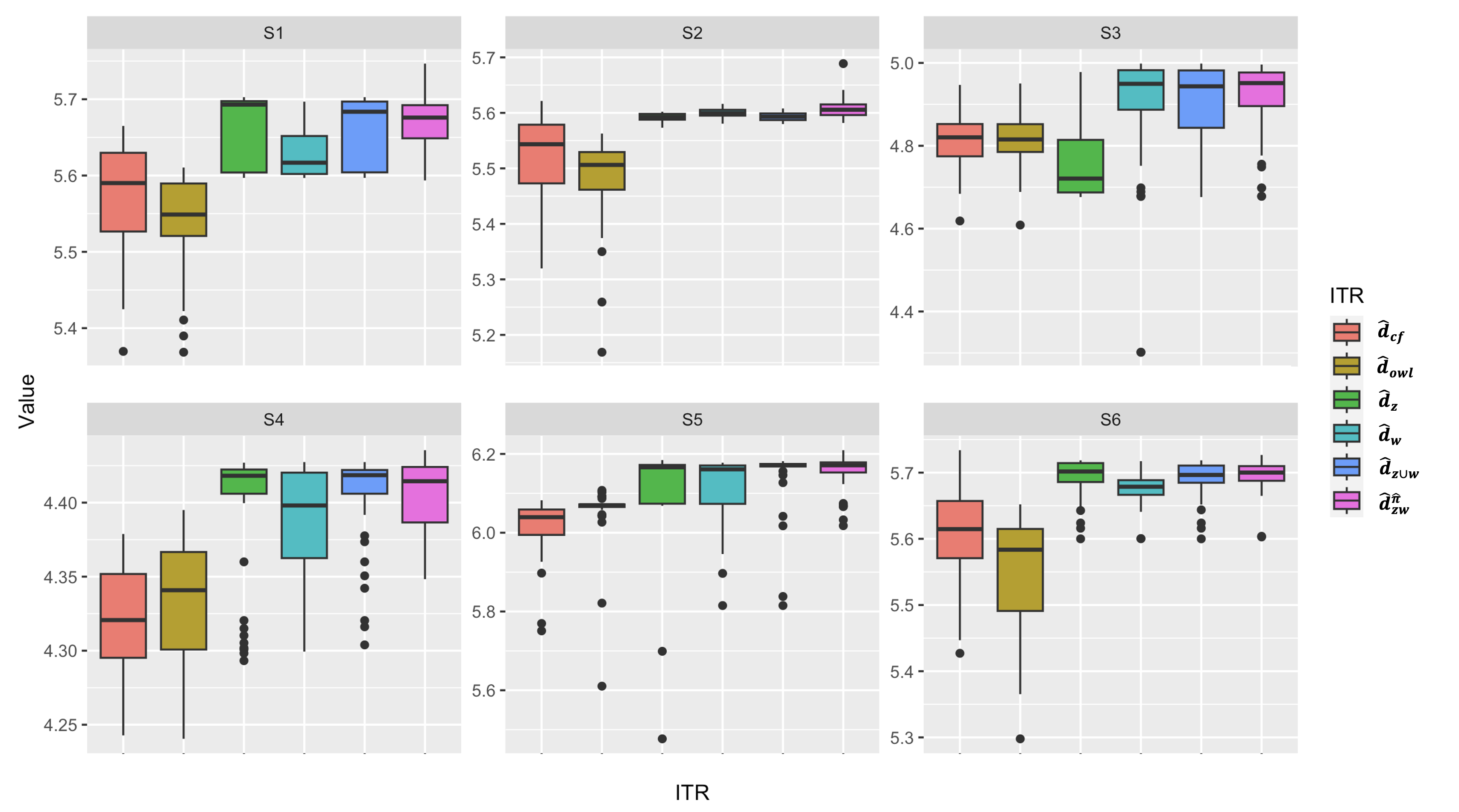
Figure 2: Boxplots of the empirical value functions (d^c​f\hat{d}_{cf} and d^o​w​l\hat{d}_{owl} denote estimated ITRs using causal forest and outcome weighted learning respectively).

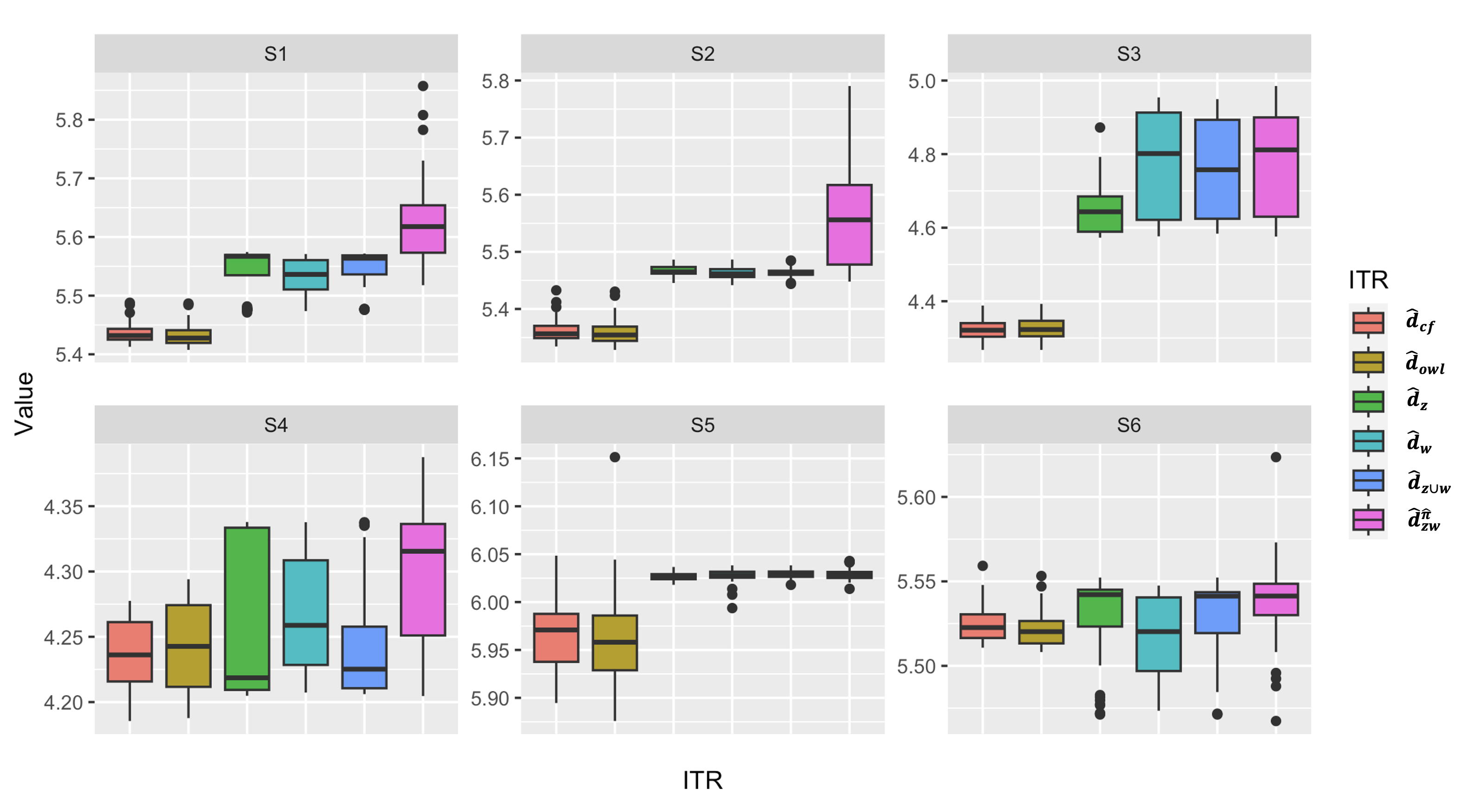
Figure 2 presents the empirical value functions of different optimal ITRs for the six scenarios. As expected, d^z,d^w,d^z∪w,\hat{d}_{z},\hat{d}_{w},\hat{d}_{z\cup w}, and d^z​wπ^\hat{d}_{zw}^{\hat{\pi}} consistently outperform d^c​f\hat{d}_{cf} and d^o​w​l\hat{d}_{owl}, which highlights their effectiveness in addressing unmeasured confounding. Meanwhile, across all scenarios, d^z​wπ^\hat{d}_{zw}^{\hat{\pi}} yields superior or comparable performance compared to the other estimated treatment regimes, which justifies the statements made in Sections 2 and 3. In addition, as can be seen in Scenario 5, all ITRs relying on the proximal causal inference framework perform similarly, which is not surprising as d^z​(X,Z)\hat{d}_{z}(X,Z) and d^w​(X,W)\hat{d}_{w}(X,W) agree for most subjects. To further underscore the robust performance of our proposed approach, we include additional results with a changed sample size and a modified behavior policy in Appendix L.

5 Real Data Application

In this section, we demonstrate the proposed optimal ITR via a real dataset originally designed to measure the effectiveness of right heart catheterization (RHC) for ill patients in intensive care units (ICU), under the Study to Understand Prognoses and Preferences for Outcomes and Risks of Treatments (SUPPORT, Connors et al. 1996). These data have been re-analyzed in a number of papers in both causal inference and survival analysis literature with assuming unconfoundednss (Cui and Tchetgen Tchetgen 2023; Tan 2006; Tan 2020; Tan 2019; Vermeulen and Vansteelandt 2015) or accounting for unmeasured confounding (Cui et al. 2023; Lin et al. 1998; Qi et al. 2023; Tchetgen Tchetgen et al. 2020; Ying et al. 2022).

There are 5735 subjects included in the dataset, in which 2184 were treated (with A=1A=1) and 3551 were untreated (with A=−1A=-1). The outcome YY is the duration from admission to death or censoring. Overall, 3817 patients survived and 1918 died within 30 days. Following Tchetgen Tchetgen et al. 2020, we collect 71 covariates including demographic factors, diagnostic information, estimated survival probability, comorbidity, vital signs, physiological status, and functional status (see Hirano and Imbens 2001 for additional discussion on covariates). Confounding in this study stems from the fact that ten physiological status measures obtained from blood tests conducted at the initial phase of admission may be susceptible to significant measurement errors. Furthermore, besides the lab measurement errors, whether other unmeasured confounding factors exist is unknown to the data analyst. Because variables measured from these tests offer only a single snapshot of the underlying physiological condition, they have the potential to act as confounding proxies. We consider a total of four settings, varying the number of selected proxies from 4 to 10. Within each setting, treatment-inducing proxies are first selected based on their strength of association with the treatment (determined through logistic regression of AA on LL), and outcome-inducing proxies are then chosen based on their association with the outcome (determined through linear regression of YY on AA and LL). Excluding the selected proxy variables, other measured covariates are included in XX. We then estimate d^z,d^w,d^z∪w\hat{d}_{z},\hat{d}_{w},\hat{d}_{z\cup w}, and d^z​wπ^\hat{d}_{zw}^{\hat{\pi}} using the SUPPORT dataset in a manner similar to that described in Section 4, with the goal optimizing the patients’ 30-day survival after their entrance into the ICU.

Refer to caption
Figure 3: Graphical representation of concordance between estimated ITRs.

The estimated value functions of our proposed ITR, alongside existing ones, are summarized in Appendix M. As can be seen, our proposed regime has the largest value among all settings. For a visual representation of the concordance between the estimated optimal ITRs, we refer to Figure 3 (results from Setting 1). The horizontal ordinate represents the 50 selected subjects and the vertical axis denotes the decisions made from corresponding ITRs. The purple and yellow blocks stand for being recommended treatment values of -1 and 1 respectively. For the subjects with purple or yellow columns, d^z​(X,Z)=d^w​(X,W)\hat{d}_{z}(X,Z)=\hat{d}_{w}(X,W), which leads to the same treatment decision for the other two ITRs. For columns with mixed colors, d^z​(X,Z)\hat{d}_{z}(X,Z) and d^w​(X,W)\hat{d}_{w}(X,W) disagree. We see that in this case d^z∪w​(X,W,Z)\hat{d}_{z\cup w}(X,W,Z) always agree with d^z​(X,Z)\hat{d}_{z}(X,Z), while d^z​wπ^​(X,W,Z)\hat{d}_{zw}^{\hat{\pi}}(X,W,Z) take values from d^z​(X,Z)\hat{d}_{z}(X,Z) or d^w​(X,W)\hat{d}_{w}(X,W) depending on the individual criteria of the subjects as indicated by π^\hat{\pi}. In addition to the quantitative analysis, we have also conducted a qualitative assessment of the estimated regime to validate its performance. For further details, please refer to Appendix M.

6 Discussion

We acknowledge several limitations of our work. Firstly, the proximal causal inference framework relies on the validity of treatment- and outcome-inducing confounding proxies. When the assumptions are violated, the proximal causal inference estimators can be biased even if unconfoundedness on the basis of measured covariates in fact holds. Therefore, one needs to carefully sort out proxies especially when domain knowledge is lacking. Secondly, while the proposed regime significantly improves upon existing methods both theoretically and numerically, it is not yet shown to be the sharpest under our considered model. It is still an open question to figure out if a more general policy class could be considered. Thirdly, our established theory provides consistency and superiority of our estimated regime. It is of great interest to derive convergence rates for Propositions 2 and 3 following Jiang 2017. In addition, it may be challenging to develop inference results for the value function of the estimated optimal treatment regimes, and further studies are warranted.

Acknowledgement

Yifan Cui was supported by the National Natural Science Foundation of China.

References

  • Angrist et al. [1996] J. D. Angrist, G. W. Imbens, and D. B. Rubin. Identification of causal effects using instrumental variables. Journal of the American statistical Association, 91(434):444–455, 1996.
  • Athey and Wager [2019] S. Athey and S. Wager. Estimating treatment effects with causal forests: An application. Observational Studies, 5(2):37–51, 2019.
  • Athey and Wager [2021] S. Athey and S. Wager. Policy learning with observational data. Econometrica, 89(1):133–161, 2021.
  • Bennett and Kallus [2023] A. Bennett and N. Kallus. Proximal reinforcement learning: Efficient off-policy evaluation in partially observed markov decision processes. Operations Research, 09 2023.
  • Chakraborty and Moodie [2013] B. Chakraborty and E. Moodie. Statistical methods for dynamic treatment regimes. Springer, 2013.
  • Chen and Christensen [2013] X. Chen and T. Christensen. Optimal uniform convergence rates for sieve nonparametric instrumental variables regression. arXiv preprint arXiv:1311.0412, 2013.
  • Chen et al. [2020] Y. Chen, D. Zeng, T. Xu, and Y. Wang. Representation learning for integrating multi-domain outcomes to optimize individualized treatment. Advances in Neural Information Processing Systems, 33:17976–17986, 2020.
  • Chen [2017] Y.-C. Chen. A tutorial on kernel density estimation and recent advances. Biostatistics & Epidemiology, 1(1):161–187, 2017.
  • Chernozhukov et al. [2018] V. Chernozhukov, D. Chetverikov, M. Demirer, E. Duflo, C. Hansen, W. Newey, and J. Robins. Double/debiased machine learning for treatment and structural parameters. The Econometrics Journal, 21(1):C1–C68, 2018.
  • Connors et al. [1996] A. F. Connors, T. Speroff, N. V. Dawson, C. Thomas, F. E. Harrell, D. Wagner, N. Desbiens, L. Goldman, A. W. Wu, R. M. Califf, et al. The effectiveness of right heart catheterization in the initial care of critically iii patients. Jama, 276(11):889–897, 1996.
  • Cui [2021] Y. Cui. Individualized decision-making under partial identification: Three perspectives, two optimality results, and one paradox. Harvard Data Science Review, 3(3), 2021.
  • Cui and Tchetgen Tchetgen [2021a] Y. Cui and E. Tchetgen Tchetgen. On a necessary and sufficient identification condition of optimal treatment regimes with an instrumental variable. Statistics & Probability Letters, 178:109180, 2021a. ISSN 0167-7152.
  • Cui and Tchetgen Tchetgen [2021b] Y. Cui and E. Tchetgen Tchetgen. A semiparametric instrumental variable approach to optimal treatment regimes under endogeneity. Journal of the American Statistical Association, 116(533):162–173, 2021b.
  • Cui and Tchetgen Tchetgen [2023] Y. Cui and E. Tchetgen Tchetgen. Selective machine learning of doubly robust functionals. Biometrika, page asad055, 2023. ISSN 1464-3510.
  • Cui et al. [2023] Y. Cui, H. Pu, X. Shi, W. Miao, and E. Tchetgen Tchetgen. Semiparametric proximal causal inference. Journal of the American Statistical Association, pages 1–12, 2023.
  • Dalmasso et al. [2020] N. Dalmasso, T. Pospisil, A. B. Lee, R. Izbicki, P. E. Freeman, and A. I. Malz. Conditional density estimation tools in python and r with applications to photometric redshifts and likelihood-free cosmological inference. Astronomy and Computing, 30:100362, 2020.
  • Dikkala et al. [2020] N. Dikkala, G. Lewis, L. Mackey, and V. Syrgkanis. Minimax estimation of conditional moment models. Advances in Neural Information Processing Systems, 33:12248–12262, 2020.
  • Dinh et al. [2016] L. Dinh, J. Sohl-Dickstein, and S. Bengio. Density estimation using real nvp. arXiv preprint arXiv:1605.08803, 2016.
  • Dukes et al. [2023] O. Dukes, I. Shpitser, and E. J. Tchetgen Tchetgen. Proximal mediation analysis. Biometrika, page asad015, 03 2023. ISSN 1464-3510.
  • Galie et al. [2009] N. Galie, M. M. Hoeper, M. Humbert, A. Torbicki, J.-L. Vachiery, J. A. Barbera, M. Beghetti, P. Corris, S. Gaine, J. S. Gibbs, et al. Guidelines for the diagnosis and treatment of pulmonary hypertension: the task force for the diagnosis and treatment of pulmonary hypertension of the european society of cardiology (esc) and the european respiratory society (ers), endorsed by the international society of heart and lung transplantation (ishlt). European heart journal, 30(20):2493–2537, 2009.
  • Ghassami et al. [2022] A. Ghassami, A. Ying, I. Shpitser, and E. Tchetgen Tchetgen. Minimax kernel machine learning for a class of doubly robust functionals with application to proximal causal inference. In International Conference on Artificial Intelligence and Statistics, pages 7210–7239. PMLR, 2022.
  • Ghassami et al. [2023] A. Ghassami, I. Shpitser, and E. T. Tchetgen. Partial identification of causal effects using proxy variables. arXiv preprint arXiv:2304.04374, 2023.
  • Han [2023] S. Han. Optimal dynamic treatment regimes and partial welfare ordering. Journal of the American Statistical Association, pages 1–11, 2023.
  • Hirano and Imbens [2001] K. Hirano and G. W. Imbens. Estimation of causal effects using propensity score weighting: An application to data on right heart catheterization. Health Services and Outcomes research methodology, 2(3):259–278, 2001.
  • Imbens and Angrist [1994] G. W. Imbens and J. D. Angrist. Identification and estimation of local average treatment effects. Econometrica, 62(2):467–475, 1994. ISSN 00129682, 14680262.
  • Jiang et al. [2019] B. Jiang, R. Song, J. Li, and D. Zeng. Entropy learning for dynamic treatment regimes. Statistica Sinica, 29(4):1633, 2019.
  • Jiang [2017] H. Jiang. Uniform convergence rates for kernel density estimation. In International Conference on Machine Learning, pages 1694–1703. PMLR, 2017.
  • Kallus et al. [2021] N. Kallus, X. Mao, and M. Uehara. Causal inference under unmeasured confounding with negative controls: A minimax learning approach. arXiv preprint arXiv:2103.14029, 2021.
  • Kitagawa and Tetenov [2018] T. Kitagawa and A. Tetenov. Who should be treated? empirical welfare maximization methods for treatment choice. Econometrica, 86(2):591–616, 2018.
  • Kompa et al. [2022] B. Kompa, D. Bellamy, T. Kolokotrones, A. Beam, et al. Deep learning methods for proximal inference via maximum moment restriction. Advances in Neural Information Processing Systems, 35:11189–11201, 2022.
  • Kosorok and Laber [2019] M. R. Kosorok and E. B. Laber. Precision medicine. Annual Review of Statistics and Its Application, 6:263–286, 2019.
  • Kress et al. [1989] R. Kress, V. Maz’ya, and V. Kozlov. Linear integral equations, volume 82. Springer, 1989.
  • Kuroki and Pearl [2014] M. Kuroki and J. Pearl. Measurement bias and effect restoration in causal inference. Biometrika, 101(2):423–437, 2014.
  • Li et al. [2023] K. Q. Li, X. Shi, W. Miao, and E. Tchetgen Tchetgen. Double negative control inference in test-negative design studies of vaccine effectiveness. Journal of the American Statistical Association, pages 1–12, 2023.
  • Liao et al. [2021] L. Liao, Z. Fu, Z. Yang, Y. Wang, M. Kolar, and Z. Wang. Instrumental variable value iteration for causal offline reinforcement learning. arXiv preprint arXiv:2102.09907, 2021.
  • Lin et al. [1998] D. Y. Lin, B. M. Psaty, and R. A. Kronmal. Assessing the sensitivity of regression results to unmeasured confounders in observational studies. Biometrics, pages 948–963, 1998.
  • Mastouri et al. [2021] A. Mastouri, Y. Zhu, L. Gultchin, A. Korba, R. Silva, M. Kusner, A. Gretton, and K. Muandet. Proximal causal learning with kernels: Two-stage estimation and moment restriction. In International Conference on Machine Learning, pages 7512–7523. PMLR, 2021.
  • Miao et al. [2018a] W. Miao, Z. Geng, and E. J. Tchetgen Tchetgen. Identifying causal effects with proxy variables of an unmeasured confounder. Biometrika, 105(4):987–993, 2018a.
  • Miao et al. [2018b] W. Miao, X. Shi, and E. Tchetgen Tchetgen. A confounding bridge approach for double negative control inference on causal effects. arXiv preprint arXiv:1808.04945, 2018b.
  • Miao et al. [2022] W. Miao, W. Hu, E. L. Ogburn, and X.-H. Zhou. Identifying effects of multiple treatments in the presence of unmeasured confounding. Journal of the American Statistical Association, pages 1–15, 2022.
  • Murphy [2003] S. A. Murphy. Optimal dynamic treatment regimes. Journal of the Royal Statistical Society: Series B (Statistical Methodology), 65(2):331–355, 2003.
  • Nadaraya [1964] E. A. Nadaraya. On estimating regression. Theory of Probability & Its Applications, 9(1):141–142, 1964.
  • Pu and Zhang [2021] H. Pu and B. Zhang. Estimating optimal treatment rules with an instrumental variable: A partial identification learning approach. Journal of the Royal Statistical Society: Series B (Statistical Methodology), 83(2):318–345, 2021.
  • Qi et al. [2023] Z. Qi, R. Miao, and X. Zhang. Proximal learning for individualized treatment regimes under unmeasured confounding. Journal of the American Statistical Association, pages 1–14, 2023.
  • Qian and Murphy [2011] M. Qian and S. A. Murphy. Performance guarantees for individualized treatment rules. Annals of Statistics, 39(2):1180, 2011.
  • Qiu et al. [2021] H. Qiu, M. Carone, E. Sadikova, M. Petukhova, R. C. Kessler, and A. Luedtke. Optimal individualized decision rules using instrumental variable methods. Journal of the American Statistical Association, 116(533):174–191, 2021.
  • Raghu et al. [2017] A. Raghu, M. Komorowski, L. A. Celi, P. Szolovits, and M. Ghassemi. Continuous state-space models for optimal sepsis treatment: a deep reinforcement learning approach. In Machine Learning for Healthcare Conference, pages 147–163. PMLR, 2017.
  • Robins [1986] J. Robins. A new approach to causal inference in mortality studies with a sustained exposure period—application to control of the healthy worker survivor effect. Mathematical modelling, 7(9-12):1393–1512, 1986.
  • Robins [1994] J. M. Robins. Correcting for non-compliance in randomized trials using structural nested mean models. Communications in Statistics: Theory and Methods, 23(8):2379–2412, 1994.
  • Robins [1997] J. M. Robins. Causal inference from complex longitudinal data. In Latent variable modeling and applications to causality, pages 69–117. Springer, 1997.
  • Robins et al. [1994] J. M. Robins, A. Rotnitzky, and L. P. Zhao. Estimation of regression coefficients when some regressors are not always observed. Journal of the American statistical Association, 89(427):846–866, 1994.
  • Rosenbaum and Rubin [1983] P. R. Rosenbaum and D. B. Rubin. The central role of the propensity score in observational studies for causal effects. Biometrika, 70(1):41–55, 1983.
  • Rotnitzky et al. [1998] A. Rotnitzky, J. M. Robins, and D. O. Scharfstein. Semiparametric regression for repeated outcomes with nonignorable nonresponse. Journal of the American Statistical Association, 93(444):1321–1339, 1998.
  • Scharfstein et al. [1999] D. O. Scharfstein, A. Rotnitzky, and J. M. Robins. Adjusting for nonignorable drop-out using semiparametric nonresponse models. Journal of the American Statistical Association, 94(448):1096–1120, 1999.
  • Scott [2015] D. W. Scott. Multivariate density estimation: theory, practice, and visualization. John Wiley & Sons, 2015.
  • Shi et al. [2020a] X. Shi, W. Miao, J. C. Nelson, and E. J. Tchetgen Tchetgen. Multiply robust causal inference with double-negative control adjustment for categorical unmeasured confounding. Journal of the Royal Statistical Society: Series B (Statistical Methodology), 82(2):521–540, 2020a.
  • Shi et al. [2020b] X. Shi, W. Miao, and E. Tchetgen Tchetgen. A selective review of negative control methods in epidemiology. Current Epidemiology Reports, 7(4):190–202, 2020b.
  • Shi et al. [2021] X. Shi, W. Miao, M. Hu, and E. Tchetgen Tchetgen. Theory for identification and inference with synthetic controls: a proximal causal inference framework. arXiv preprint arXiv:2108.13935, 2021.
  • Shpitser et al. [2023] I. Shpitser, Z. Wood-Doughty, and E. J. T. Tchetgen. The proximal id algorithm. Journal of Machine Learning Research, 23:1–46, 2023.
  • Singh [2020] R. Singh. Kernel methods for unobserved confounding: Negative controls, proxies, and instruments. arXiv preprint arXiv:2012.10315, 2020.
  • Sohn et al. [2015] K. Sohn, H. Lee, and X. Yan. Learning structured output representation using deep conditional generative models. Advances in Neural Information Processing Systems, 28, 2015.
  • Stensrud and Sarvet [2022] M. J. Stensrud and A. L. Sarvet. Optimal regimes for algorithm-assisted human decision-making. arXiv preprint arXiv:2203.03020, 2022.
  • Sverdrup and Cui [2023] E. Sverdrup and Y. Cui. Proximal causal learning of heterogeneous treatment effects. In International Conference on Machine Learning, 2023.
  • Tan [2006] Z. Tan. A distributional approach for causal inference using propensity scores. Journal of the American Statistical Association, 101(476):1619–1637, 2006.
  • Tan [2019] Z. Tan. Regularized calibrated estimation of propensity scores with model misspecification and high-dimensional data. Biometrika, 107(1):137–158, 12 2019. ISSN 0006-3444.
  • Tan [2020] Z. Tan. Model-assisted inference for treatment effects using regularized calibrated estimation with high-dimensional data. The Annals of Statistics, 48(2):811–837, 2020.
  • Tchetgen Tchetgen [2014] E. Tchetgen Tchetgen. The control outcome calibration approach for causal inference with unobserved confounding. American journal of epidemiology, 179(5):633–640, 2014.
  • Tchetgen Tchetgen et al. [2020] E. J. Tchetgen Tchetgen, A. Ying, Y. Cui, X. Shi, and W. Miao. An introduction to proximal causal learning. arXiv preprint arXiv:2009.10982, 2020.
  • Tsiatis et al. [2019] A. A. Tsiatis, M. Davidian, S. T. Holloway, and E. B. Laber. Dynamic treatment regimes: Statistical methods for precision medicine. Chapman and Hall/CRC, 2019.
  • Vermeulen and Vansteelandt [2015] K. Vermeulen and S. Vansteelandt. Bias-reduced doubly robust estimation. Journal of the American Statistical Association, 110(511):1024–1036, 2015.
  • Wang et al. [2022] J. Wang, Z. Qi, and C. Shi. Blessing from experts: Super reinforcement learning in confounded environments. arXiv preprint arXiv:2209.15448, 2022.
  • Wu et al. [2019] P. Wu, D. Zeng, and Y. Wang. Matched learning for optimizing individualized treatment strategies using electronic health records. Journal of the American Statistical Association, 2019.
  • Ying et al. [2022] A. Ying, Y. Cui, and E. J. T. Tchetgen. Proximal causal inference for marginal counterfactual survival curves. arXiv preprint arXiv:2204.13144, 2022.
  • Ying et al. [2023] A. Ying, W. Miao, X. Shi, and E. J. T. Tchetgen. Proximal causal inference for complex longitudinal studies. Journal of the Royal Statistical Society Series B: Statistical Methodology, 2023. In press.
  • Yoon et al. [2018] J. Yoon, J. Jordon, and M. Van Der Schaar. Ganite: Estimation of individualized treatment effects using generative adversarial nets. International Conference on Learning Representations, 2018.
  • Zhang et al. [2012] B. Zhang, A. A. Tsiatis, E. B. Laber, and M. Davidian. A robust method for estimating optimal treatment regimes. Biometrics, 68(4):1010–1018, 2012.
  • Zhao et al. [2012] Y. Zhao, D. Zeng, A. J. Rush, and M. R. Kosorok. Estimating individualized treatment rules using outcome weighted learning. Journal of the American Statistical Association, 107(499):1106–1118, 2012.
  • Zhao et al. [2019] Y.-Q. Zhao, E. B. Laber, Y. Ning, S. Saha, and B. E. Sands. Efficient augmentation and relaxation learning for individualized treatment rules using observational data. Journal of Machine Learning Research, 20(1):1821–1843, 2019.

Supplementary Material

Appendix A Proof of identification (3)

The proof is straightforward. We state it here for clarity and completeness. Note that

𝕀{dz∪w(X,W,Z)=1}=𝕀{dz∪w∈𝒟𝒵}𝕀{dz∪w(X,Z)=1}+𝕀{dz∪w∈𝒟𝒲}𝕀{dz∪w(X,W)=1},\mathbb{I}\{d_{z\cup w}(X,W,Z)=1\}=\mathbb{I}\{d_{z\cup w}\in\mathcal{D}_{\mathcal{Z}}\}\mathbb{I}\{d_{z\cup w}(X,Z)=1\}+\mathbb{I}\{d_{z\cup w}\in\mathcal{D}_{\mathcal{W}}\}\mathbb{I}\{d_{z\cup w}(X,W)=1\},
𝕀{dz∪w(X,W,Z)=−1}=𝕀{dz∪w∈𝒟𝒵}𝕀{dz∪w(X,Z)=−1}+𝕀{dz∪w∈𝒟𝒲}𝕀{dz∪w(X,W)=−1}.\mathbb{I}\{d_{z\cup w}(X,W,Z)=-1\}=\mathbb{I}\{d_{z\cup w}\in\mathcal{D}_{\mathcal{Z}}\}\mathbb{I}\{d_{z\cup w}(X,Z)=-1\}+\mathbb{I}\{d_{z\cup w}\in\mathcal{D}_{\mathcal{W}}\}\mathbb{I}\{d_{z\cup w}(X,W)=-1\}.

Therefore, we have

𝔼[Y(1)𝕀{dz∪w(X,W,Z)=1}]\displaystyle\mathbb{E}[Y(1)\mathbb{I}\{d_{z\cup w}(X,W,Z)=1\}] =𝔼[Y(1)𝕀{dz∪w∈𝒟𝒵}𝕀{dz∪w(X,Z)=1}\displaystyle=\mathbb{E}[Y(1)\mathbb{I}\{d_{z\cup w}\in\mathcal{D}_{\mathcal{Z}}\}\mathbb{I}\{d_{z\cup w}(X,Z)=1\}
+Y(1)𝕀{dz∪w∈𝒟𝒲}𝕀{dz∪w(X,W)=1}]\displaystyle+Y(1)\mathbb{I}\{d_{z\cup w}\in\mathcal{D}_{\mathcal{W}}\}\mathbb{I}\{d_{z\cup w}(X,W)=1\}]
=𝕀{dz∪w∈𝒟𝒵}𝔼[Y(1)𝕀{dz∪w(X,Z)=1}]\displaystyle=\mathbb{I}\{d_{z\cup w}\in\mathcal{D}_{\mathcal{Z}}\}\mathbb{E}[Y(1)\mathbb{I}\{d_{z\cup w}(X,Z)=1\}]
+𝕀{dz∪w∈𝒟𝒲}𝔼[Y(1)𝕀{dz∪w(X,W)=1}].\displaystyle+\mathbb{I}\{d_{z\cup w}\in\mathcal{D}_{\mathcal{W}}\}\ \mathbb{E}[Y(1)\mathbb{I}\{d_{z\cup w}(X,W)=1\}].

Similarly,

𝔼[Y(−1)𝕀{dz∪w(X,W,Z)=−1}]\displaystyle\mathbb{E}[Y(-1)\mathbb{I}\{d_{z\cup w}(X,W,Z)=-1\}] =𝕀{dz∪w∈𝒟𝒵}𝔼[Y(−1)𝕀{dz∪w(X,Z)=−1}]\displaystyle=\mathbb{I}\{d_{z\cup w}\in\mathcal{D}_{\mathcal{Z}}\}\mathbb{E}[Y(-1)\mathbb{I}\{d_{z\cup w}(X,Z)=-1\}]
+𝕀{dz∪w∈𝒟𝒲}𝔼[Y(−1)𝕀{dz∪w(X,W)=−1}].\displaystyle+\mathbb{I}\{d_{z\cup w}\in\mathcal{D}_{\mathcal{W}}\}\ \mathbb{E}[Y(-1)\mathbb{I}\{d_{z\cup w}(X,W)=-1\}].

So

V⁡(dz∪w)\displaystyle V(d_{z\cup w}) =𝔼[Y(1)𝕀{dz∪w(X,W,Z)=1}]+𝔼[Y(−1)𝕀{dz∪w(X,W,Z)=−1}]\displaystyle=\mathbb{E}[Y(1)\mathbb{I}\{d_{z\cup w}(X,W,Z)=1\}]+\mathbb{E}[Y(-1)\mathbb{I}\{d_{z\cup w}(X,W,Z)=-1\}]
=𝕀{dz∪w∈𝒟𝒵}𝔼[Y(1)𝕀{dz∪w(X,Z)=1}+Y(−1)𝕀{dz∪w(X,Z)=−1}]\displaystyle=\mathbb{I}\{d_{z\cup w}\in\mathcal{D}_{\mathcal{Z}}\}\mathbb{E}[Y(1)\mathbb{I}\{d_{z\cup w}(X,Z)=1\}+Y(-1)\mathbb{I}\{d_{z\cup w}(X,Z)=-1\}]
+𝕀{dz∪w∈𝒟𝒲}𝔼[Y(1)𝕀{dz∪w(X,W)=1}+Y(−1)𝕀{dz∪w(X,W)=−1}]\displaystyle+\mathbb{I}\{d_{z\cup w}\in\mathcal{D}_{\mathcal{W}}\}\mathbb{E}[Y(1)\mathbb{I}\{d_{z\cup w}(X,W)=1\}+Y(-1)\mathbb{I}\{d_{z\cup w}(X,W)=-1\}]
=𝕀{dz∪w∈𝒟𝒵}𝔼[h(W,dz∪w(X,Z),X)]+𝕀{dz∪w∈𝒟𝒲}𝔼[Yq(Z,A,X)𝕀{dz∪w(X,W)=A}],\displaystyle=\mathbb{I}\{d_{z\cup w}\in\mathcal{D}_{\mathcal{Z}}\}\mathbb{E}[h(W,d_{z\cup w}(X,Z),X)]+\mathbb{I}\{d_{z\cup w}\in\mathcal{D}_{\mathcal{W}}\}\mathbb{E}[Yq(Z,A,X)\mathbb{I}\{d_{z\cup w}(X,W)=A\}],

where the last equality holds due to identification results (1) and (2).

Appendix B Proof of Theorem 1

Recall that V(dz​wπ)=𝔼[Y(1)𝕀{dz​wπ(X,W,Z)=1}+Y(−1)𝕀{dz​wπ(X,W,Z)=−1}]V(d_{zw}^{\pi})=\mathbb{E}[Y(1)\mathbb{I}\{d_{zw}^{\pi}(X,W,Z)=1\}+Y(-1)\mathbb{I}\{d_{zw}^{\pi}(X,W,Z)=-1\}], we essentially need to consider the first term 𝔼[Y(1)𝕀{dz​wπ(X,W,Z)=1}]\mathbb{E}[Y(1)\mathbb{I}\{d_{zw}^{\pi}(X,W,Z)=1\}]. Note that

𝕀{dz​wπ(X,W,Z)=1}=𝕀{π(X)=1}𝕀{dz(X,Z)=1}+𝕀{π(X)=0}𝕀{dw(X,W)=1},\mathbb{I}\{d_{zw}^{\pi}(X,W,Z)=1\}=\mathbb{I}\{\pi(X)=1\}\mathbb{I}\{d_{z}(X,Z)=1\}+\mathbb{I}\{\pi(X)=0\}\mathbb{I}\{d_{w}(X,W)=1\},

we have

𝔼[Y(1)𝕀{dz​wπ(X,W,Z)=1}]\displaystyle\mathbb{E}[Y(1)\mathbb{I}\{d_{zw}^{\pi}(X,W,Z)=1\}] =𝔼[Y(1)𝕀{π(X)=1}𝕀{dz(X,Z)=1}+Y(1)𝕀{π(X)=0}𝕀{dw(X,W)=1}]\displaystyle=\mathbb{E}[Y(1)\mathbb{I}\{\pi(X)=1\}\mathbb{I}\{d_{z}(X,Z)=1\}+Y(1)\mathbb{I}\{\pi(X)=0\}\mathbb{I}\{d_{w}(X,W)=1\}]
=𝔼[𝕀{π(X)=1}𝔼[Y(1)𝕀{dz(X,Z)=1}|X]\displaystyle=\mathbb{E}[\mathbb{I}\{\pi(X)=1\}\mathbb{E}[Y(1)\mathbb{I}\{d_{z}(X,Z)=1\}|X]
+𝕀{π(X)=0}𝔼[Y(1)𝕀{dw(X,W)=1}|X]].\displaystyle+\mathbb{I}\{\pi(X)=0\}\mathbb{E}[Y(1)\mathbb{I}\{d_{w}(X,W)=1\}|X]].

By leveraging the outcome confounding bridge, we have

𝔼[Y(1)𝕀{dz(X,Z)=1}|X]\displaystyle\mathbb{E}[Y(1)\mathbb{I}\{d_{z}(X,Z)=1\}|X] =𝔼[𝔼[Y(1)|X,Z]𝕀{dz(X,Z)=1}|X]\displaystyle=\mathbb{E}[\mathbb{E}[Y(1)|X,Z]\mathbb{I}\{d_{z}(X,Z)=1\}|X]
=𝔼[𝔼[𝔼[Y(1)|X,Z,U]|X,Z]𝕀{dz(X,Z)=1}|X]\displaystyle=\mathbb{E}[\mathbb{E}[\mathbb{E}[Y(1)|X,Z,U]|X,Z]\mathbb{I}\{d_{z}(X,Z)=1\}|X]
=𝔼[𝔼[𝔼[Y|X,U,A=1]|X,Z]𝕀{dz(X,Z)=1}|X]\displaystyle=\mathbb{E}[\mathbb{E}[\mathbb{E}[Y|X,U,A=1]|X,Z]\mathbb{I}\{d_{z}(X,Z)=1\}|X]
=𝔼[𝔼[𝔼[h(W,1,X)|X,U]|X,Z]𝕀{dz(X,Z)=1}|X]\displaystyle=\mathbb{E}[\mathbb{E}[\mathbb{E}[h(W,1,X)|X,U]|X,Z]\mathbb{I}\{d_{z}(X,Z)=1\}|X]
=𝔼[𝔼[𝔼[h(W,1,X)|X,Z,U]|X,Z]𝕀{dz(X,Z)=1}|X]\displaystyle=\mathbb{E}[\mathbb{E}[\mathbb{E}[h(W,1,X)|X,Z,U]|X,Z]\mathbb{I}\{d_{z}(X,Z)=1\}|X]
=𝔼[h(W,1,X)𝕀{dz(X,Z)=1}|X],\displaystyle=\mathbb{E}[h(W,1,X)\mathbb{I}\{d_{z}(X,Z)=1\}|X],

where the third equality is due to Assumption 1, the fourth equality can be verified by Theorem 1 in Miao et al. 2018a under Assumptions 2 and 3, and the fifth equality is due to Assumption 1. Moreover, by leveraging the treatment confounding bridge, we have

𝔼[Y(1)𝕀{dw(X,W)=1}|X]\displaystyle\mathbb{E}[Y(1)\mathbb{I}\{d_{w}(X,W)=1\}|X] =𝔼[𝔼[Y(1)|X,W]𝕀{dw(X,W)=1}|X]\displaystyle=\mathbb{E}[\mathbb{E}[Y(1)|X,W]\mathbb{I}\{d_{w}(X,W)=1\}|X]
=𝔼[𝔼[𝔼[Y(1)|X,W,U]|X,W]𝕀{dw(X,W)=1}|X]\displaystyle=\mathbb{E}[\mathbb{E}[\mathbb{E}[Y(1)|X,W,U]|X,W]\mathbb{I}\{d_{w}(X,W)=1\}|X]
=𝔼[𝔼[𝔼[Y(1)|X,W,U,A=1]|X,W]𝕀{dw(X,W)=1}|X]\displaystyle=\mathbb{E}[\mathbb{E}[\mathbb{E}[Y(1)|X,W,U,A=1]|X,W]\mathbb{I}\{d_{w}(X,W)=1\}|X]
=𝔼[𝔼[𝔼[Y(1)|X,W,U,A=1]𝔼[q(Z,1,X)|X,U,A=1]\displaystyle=\mathbb{E}[\mathbb{E}[\mathbb{E}[Y(1)|X,W,U,A=1]\mathbb{E}[q(Z,1,X)|X,U,A=1]
ℙ(A=1|X,U)|X,W]𝕀{dw(X,W)=1}|X]\displaystyle\ \ \ \mathbb{P}(A=1|X,U)|X,W]\mathbb{I}\{d_{w}(X,W)=1\}|X]
=𝔼[𝔼[𝔼[Yq(Z,1,X)𝕀{A=1}|X,U,W]|X,W]𝕀{dw(X,W)=1}|X]\displaystyle=\mathbb{E}[\mathbb{E}[\mathbb{E}[Yq(Z,1,X)\mathbb{I}\{A=1\}|X,U,W]|X,W]\mathbb{I}\{d_{w}(X,W)=1\}|X]
=𝔼[Yq(Z,1,X)𝕀{A=1}𝕀{dw(X,W)=1}|X],\displaystyle=\mathbb{E}[Yq(Z,1,X)\mathbb{I}\{A=1\}\mathbb{I}\{d_{w}(X,W)=1\}|X],

where the third equality is due to Assumption 1, the fourth equality is implied by Theorem 2.2 of Cui et al. 2023 under Assumptions 4 and 5, and the fifth equality is due to Assumption 1. Therefore,

𝔼[Y(1)𝕀{dz​wπ(X,W,Z)=1}]\displaystyle\mathbb{E}[Y(1)\mathbb{I}\{d_{zw}^{\pi}(X,W,Z)=1\}] =𝔼[𝕀{π(X)=1}𝔼[Y(1)𝕀{dz(X,Z)=1}|X]\displaystyle=\mathbb{E}[\mathbb{I}\{\pi(X)=1\}\mathbb{E}[Y(1)\mathbb{I}\{d_{z}(X,Z)=1\}|X]
+𝕀{π(X)=0}𝔼[Y(1)𝕀{dw(X,W)=1}|X]]\displaystyle+\mathbb{I}\{\pi(X)=0\}\mathbb{E}[Y(1)\mathbb{I}\{d_{w}(X,W)=1\}|X]]
=𝔼[𝕀{π(X)=1}𝔼[h(W,1,X)𝕀{dz(X,Z)=1}|X]\displaystyle=\mathbb{E}[\mathbb{I}\{\pi(X)=1\}\mathbb{E}[h(W,1,X)\mathbb{I}\{d_{z}(X,Z)=1\}|X]
+𝕀{π(X)=0}𝔼[Yq(Z,1,X)𝕀{A=1}𝕀{dw(X,W)=1}|X]]\displaystyle+\mathbb{I}\{\pi(X)=0\}\mathbb{E}[Yq(Z,1,X)\mathbb{I}\{A=1\}\mathbb{I}\{d_{w}(X,W)=1\}|X]]
=𝔼[𝕀{π(X)=1}h(W,1,X)𝕀{dz(X,Z)=1}\displaystyle=\mathbb{E}[\mathbb{I}\{\pi(X)=1\}h(W,1,X)\mathbb{I}\{d_{z}(X,Z)=1\}
+𝕀{π(X)=0}Yq(Z,1,X)𝕀{A=1}𝕀{dw(X,W)=1}].\displaystyle+\mathbb{I}\{\pi(X)=0\}Yq(Z,1,X)\mathbb{I}\{A=1\}\mathbb{I}\{d_{w}(X,W)=1\}]. (10)

Similarly, as

𝕀{dz​wπ(X,W,Z)=−1}=𝕀{π(X)=1}𝕀{dz(X,Z)=−1}+𝕀{π(X)=0}𝕀{dw(X,W)=−1},\mathbb{I}\{d_{zw}^{\pi}(X,W,Z)=-1\}=\mathbb{I}\{\pi(X)=1\}\mathbb{I}\{d_{z}(X,Z)=-1\}+\mathbb{I}\{\pi(X)=0\}\mathbb{I}\{d_{w}(X,W)=-1\},

we have

𝔼[Y(−1)𝕀{dz​wπ(X,W,Z)=−1}]\displaystyle\mathbb{E}[Y(-1)\mathbb{I}\{d_{zw}^{\pi}(X,W,Z)=-1\}]
=𝔼[𝕀{π(X)=1}h(W,−1,X)𝕀{dz(X,Z)=−1}\displaystyle=\mathbb{E}[\mathbb{I}\{\pi(X)=1\}h(W,-1,X)\mathbb{I}\{d_{z}(X,Z)=-1\}
+𝕀{π(X)=0}Yq(Z,−1,X)𝕀{A=−1}𝕀{dw(X,W)=−1}].\displaystyle+\mathbb{I}\{\pi(X)=0\}Yq(Z,-1,X)\mathbb{I}\{A=-1\}\mathbb{I}\{d_{w}(X,W)=-1\}]. (11)

Combining (B) and (B), we have

V⁡(dz​wπ)\displaystyle V(d_{zw}^{\pi}) =𝔼[Y(1)𝕀{dz​wπ(X,W,Z)=1}+Y(−1)𝕀{dz​wπ(X,W,Z)=−1}]\displaystyle=\mathbb{E}[Y(1)\mathbb{I}\{d_{zw}^{\pi}(X,W,Z)=1\}+Y(-1)\mathbb{I}\{d_{zw}^{\pi}(X,W,Z)=-1\}]
=𝔼[𝕀{π(X)=1}h(W,1,X)𝕀{dz(X,Z)=1}\displaystyle=\mathbb{E}[\mathbb{I}\{\pi(X)=1\}h(W,1,X)\mathbb{I}\{d_{z}(X,Z)=1\}
+𝕀{π(X)=0}Yq(Z,1,X)𝕀{A=1}𝕀{dw(X,W)=1}\displaystyle+\mathbb{I}\{\pi(X)=0\}Yq(Z,1,X)\mathbb{I}\{A=1\}\mathbb{I}\{d_{w}(X,W)=1\}
+𝕀{π(X)=1}h(W,−1,X)𝕀{dz(X,Z)=−1}\displaystyle+\mathbb{I}\{\pi(X)=1\}h(W,-1,X)\mathbb{I}\{d_{z}(X,Z)=-1\}
+𝕀{π(X)=0}Yq(Z,−1,X)𝕀{A=−1}𝕀{dw(X,W)=−1}]\displaystyle+\mathbb{I}\{\pi(X)=0\}Yq(Z,-1,X)\mathbb{I}\{A=-1\}\mathbb{I}\{d_{w}(X,W)=-1\}]
=𝔼[𝕀{π(X)=1}h(W,dz(X,Z),X)+𝕀{π(X)=0}Yq(Z,A,X)𝕀{dw(X,W)=A}]\displaystyle=\mathbb{E}[\mathbb{I}\{\pi(X)=1\}h(W,d_{z}(X,Z),X)+\mathbb{I}\{\pi(X)=0\}Yq(Z,A,X)\mathbb{I}\{d_{w}(X,W)=A\}]
=𝔼[π(X)h(W,dz(X,Z),X)+(1−π(X))Yq(Z,A,X)𝕀{dw(X,W)=A}],\displaystyle=\mathbb{E}[\pi(X)h(W,d_{z}(X,Z),X)+(1-\pi(X))Yq(Z,A,X)\mathbb{I}\{d_{w}(X,W)=A\}],

which completes the proof.

Appendix C Proof of Theorem 2

For any dz∈𝒟𝒵d_{z}\in\mathcal{D}_{\mathcal{Z}} and dw∈𝒟𝒲d_{w}\in\mathcal{D}_{\mathcal{W}}, we have

V⁡(dz​wπ¯)\displaystyle V(d_{zw}^{\bar{\pi}}) =𝔼[π¯(X;dz,dw)h(W,dz(X,Z),X)+(1−π¯(X;dz,dw))Yq(Z,A,X)𝕀{dw(X,W)=A}]\displaystyle=\mathbb{E}[\bar{\pi}(X;d_{z},d_{w})h(W,d_{z}(X,Z),X)+(1-\bar{\pi}(X;d_{z},d_{w}))Yq(Z,A,X)\mathbb{I}\{d_{w}(X,W)=A\}]
=𝔼[π¯(X;dz,dw)𝔼[h(W,dz(X,Z),X)|X]+(1−π¯(X;dz,dw))𝔼[Yq(Z,A,X)𝕀{dw(X,W)=A}|X]]\displaystyle=\mathbb{E}[\bar{\pi}(X;d_{z},d_{w})\mathbb{E}[h(W,d_{z}(X,Z),X)|X]+(1-\bar{\pi}(X;d_{z},d_{w}))\mathbb{E}[Yq(Z,A,X)\mathbb{I}\{d_{w}(X,W)=A\}|X]]
=𝔼[max{𝔼[h(W,dz(X,Z),X)|X],𝔼[Yq(Z,A,X)𝕀{dw(X,W)=A}|X]}],\displaystyle=\mathbb{E}[\max\{\mathbb{E}[h(W,d_{z}(X,Z),X)|X],\mathbb{E}[Yq(Z,A,X)\mathbb{I}\{d_{w}(X,W)=A\}|X]\}],

where the last equality is due to the definition of π¯​(X,dz,dw)\bar{\pi}(X;d_{z},d_{w}). As

max{𝔼[h(W,dz(X,Z),X)|X],𝔼[Yq(Z,A,X)𝕀{dw(X,W)=A}|X]}≥𝔼[h(W,dz(X,Z),X)|X],\max\{\mathbb{E}[h(W,d_{z}(X,Z),X)|X],\mathbb{E}[Yq(Z,A,X)\mathbb{I}\{d_{w}(X,W)=A\}|X]\}\geq\mathbb{E}[h(W,d_{z}(X,Z),X)|X],

and

max{𝔼[h(W,dz(X,Z),X)|X],𝔼[Yq(Z,A,X)𝕀{dw(X,W)=A}|X]}≥𝔼[Yq(Z,A,X)𝕀{dw(X,W)=A}|X],\displaystyle\max\{\mathbb{E}[h(W,d_{z}(X,Z),X)|X],\mathbb{E}[Yq(Z,A,X)\mathbb{I}\{d_{w}(X,W)=A\}|X]\}\geq\mathbb{E}[Yq(Z,A,X)\mathbb{I}\{d_{w}(X,W)=A\}|X],

taking expectations on both sides, we have

𝔼[max{𝔼[h(W,dz(X,Z),X)|X],𝔼[Yq(Z,A,X)𝕀{dw(X,W)=A}|X]}]\displaystyle\mathbb{E}[\max\{\mathbb{E}[h(W,d_{z}(X,Z),X)|X],\mathbb{E}[Yq(Z,A,X)\mathbb{I}\{d_{w}(X,W)=A\}|X]\}]
≥𝔼⁡[𝔼⁡[h⁡(W,dz​(X,Z),X)|X]]\displaystyle\geq\mathbb{E}[\mathbb{E}[h(W,d_{z}(X,Z),X)|X]]
=𝔼⁡[h⁡(W,dz​(X,Z),X)]\displaystyle=\mathbb{E}[h(W,d_{z}(X,Z),X)]
=V⁡(dz),\displaystyle=V(d_{z}),
𝔼[max{𝔼[h(W,dz(X,Z),X)|X],𝔼[Yq(Z,A,X)𝕀{dw(X,W)=A}|X]}]\displaystyle\mathbb{E}[\max\{\mathbb{E}[h(W,d_{z}(X,Z),X)|X],\mathbb{E}[Yq(Z,A,X)\mathbb{I}\{d_{w}(X,W)=A\}|X]\}]
≥𝔼[𝔼[Yq(Z,A,X)𝕀{dw(X,W)=A}|X]]\displaystyle\geq\mathbb{E}[\mathbb{E}[Yq(Z,A,X)\mathbb{I}\{d_{w}(X,W)=A\}|X]]
=𝔼[Yq(Z,A,X)𝕀{dw(X,W)=A}]\displaystyle=\mathbb{E}[Yq(Z,A,X)\mathbb{I}\{d_{w}(X,W)=A\}]
=V⁡(dw).\displaystyle=V(d_{w}).

Therefore, we have V⁡(dz​wπ¯)≥max⁡{V⁡(dz),V⁡(dw)}V(d_{zw}^{\bar{\pi}})\geq\max\{V(d_{z}),V(d_{w})\}.

Appendix D Proof of Corollary 1

Recall that

dz​wπ¯∗(X,W,Z)=π¯(X;dz∗,dw∗)dz∗(X,Z)+(1−π¯(X;dz∗,dw∗))dw∗(X,W),d_{zw}^{\bar{\pi}*}(X,W,Z)=\bar{\pi}(X;d_{z}^{*},d_{w}^{*})d_{z}^{*}(X,Z)+(1-\bar{\pi}(X;d_{z}^{*},d_{w}^{*}))d_{w}^{*}(X,W),

with

π¯(X;dz∗,dw∗)=𝕀{𝔼[h(W,dz∗(X,Z),X|X]≥𝔼[Yq(Z,A,X)𝕀{dw∗(X,W)=A}|X]},\bar{\pi}(X;d_{z}^{*},d_{w}^{*})=\mathbb{I}\{\mathbb{E}[h(W,d_{z}^{*}(X,Z),X|X]\geq\mathbb{E}[Yq(Z,A,X)\mathbb{I}\{d_{w}^{*}(X,W)=A\}|X]\},

we apply the result in Theorem 2, i.e.,

V(dz​wπ¯∗)≥max{V(dz∗),V(dw∗)}.V(d_{zw}^{\bar{\pi}*})\geq\max\{V(d_{z}^{*}),V(d_{w}^{*})\}.

Due to V⁡(dz∪w∗)=max⁡{V⁡(dz∗),V⁡(dw∗)}V(d_{z\cup w}^{*})=\max\{V(d_{z}^{*}),V(d_{w}^{*})\} as shown in Qi et al. 2023, we then conclude that V(dz​wπ¯∗)≥max{V(dz∗),V(dw∗),V(dz∪w∗)}.V(d_{zw}^{\bar{\pi}*})\geq\max\{V(d_{z}^{*}),V(d_{w}^{*}),V(d_{z\cup w}^{*})\}.

Appendix E Proof of Proposition 1

In the following, we show

dz​wπ¯∗∈argmaxdz​wπ∈𝒟𝒵​𝒲ΠV(dz​wπ).d_{zw}^{\bar{\pi}*}\in\arg\max_{d_{zw}^{\pi}\in\mathcal{D}_{\mathcal{ZW}}^{\Pi}}V(d_{zw}^{\pi}).

Recall that

V⁡(dz​wπ¯)\displaystyle V(d_{zw}^{\bar{\pi}}) =𝔼[π¯(X;dz,dw)h(W,dz(X,Z),X)+(1−π¯(X;dz,dw))Yq(Z,A,X)𝕀{dw(X,W)=A}]\displaystyle=\mathbb{E}[\bar{\pi}(X;d_{z},d_{w})h(W,d_{z}(X,Z),X)+(1-\bar{\pi}(X;d_{z},d_{w}))Yq(Z,A,X)\mathbb{I}\{d_{w}(X,W)=A\}]
=𝔼[π¯(X;dz,dw)𝔼[h(W,dz(X,Z),X)|X]+(1−π¯(X;dz,dw))𝔼[Yq(Z,A,X)𝕀{dw(X,W)=A}|X]]\displaystyle=\mathbb{E}[\bar{\pi}(X;d_{z},d_{w})\mathbb{E}[h(W,d_{z}(X,Z),X)|X]+(1-\bar{\pi}(X;d_{z},d_{w}))\mathbb{E}[Yq(Z,A,X)\mathbb{I}\{d_{w}(X,W)=A\}|X]]
=𝔼[max{𝔼[h(W,dz(X,Z),X)|X],𝔼[Yq(Z,A,X)𝕀{dw(X,W)=A}|X]}]\displaystyle=\mathbb{E}[\max\{\mathbb{E}[h(W,d_{z}(X,Z),X)|X],\mathbb{E}[Yq(Z,A,X)\mathbb{I}\{d_{w}(X,W)=A\}|X]\}]
≥𝔼[π(X)𝔼[h(W,dz(X,Z),X)|X]+(1−π(X))𝔼[Yq(Z,A,X)𝕀{dw(X,W)=A}|X]]\displaystyle\geq\mathbb{E}[\pi(X)\mathbb{E}[h(W,d_{z}(X,Z),X)|X]+(1-\pi(X))\mathbb{E}[Yq(Z,A,X)\mathbb{I}\{d_{w}(X,W)=A\}|X]]
=V⁡(dz​wπ),\displaystyle=V(d_{zw}^{\pi}),

for any dz∈𝒟𝒵,dw∈𝒟𝒲d_{z}\in\mathcal{D}_{\mathcal{Z}},d_{w}\in\mathcal{D}_{\mathcal{W}} and π⁡(⋅)\pi(\cdot). Therefore, we essentially need to show

dz​wπ¯∗∈argmaxdz​wπ¯∈𝒟𝒵​𝒲π¯V(dz​wπ¯),d_{zw}^{\bar{\pi}*}\in\arg\max_{d_{zw}^{\bar{\pi}}\in\mathcal{D}^{\bar{\pi}}_{\mathcal{ZW}}}V(d_{zw}^{\bar{\pi}}),

where 𝒟𝒵​𝒲π¯=△{dz​wπ¯:dz​wπ¯(X,W,Z)=π¯(X)dz(X,Z)+(1−π¯(X))dw(X,W),dz∈𝒟𝒵,dw∈𝒟𝒲}\mathcal{D}^{\bar{\pi}}_{\mathcal{ZW}}\overset{\triangle}{=}\{d_{zw}^{\bar{\pi}}:d_{zw}^{\bar{\pi}}(X,W,Z)=\bar{\pi}(X)d_{z}(X,Z)+(1-\bar{\pi}(X))d_{w}(X,W),d_{z}\in\mathcal{D}_{\mathcal{Z}},d_{w}\in\mathcal{D}_{\mathcal{W}}\}. Recall that

dz∗​(X,Z)=\displaystyle d_{z}^{*}(X,Z)= sign{𝔼[h(W,1,X)−h(W,−1,X)|X,Z]},\displaystyle\text{sign}\{\mathbb{E}[h(W,1,X)-h(W,-1,X)|X,Z]\},
dw∗​(X,W)=\displaystyle d_{w}^{*}(X,W)= sign{𝔼[Yq(Z,A,X)𝕀{A=1}−Yq(Z,A,X)𝕀{A=−1}|X,W]},\displaystyle\text{sign}\{\mathbb{E}[Yq(Z,A,X)\mathbb{I}\{A=1\}-Yq(Z,A,X)\mathbb{I}\{A=-1\}|X,W]\},

we have

𝔼[h(W,dz∗(X,Z),X)|X,Z]≥\displaystyle\mathbb{E}[h(W,d_{z}^{*}(X,Z),X)|X,Z]\geq 𝔼[h(W,dz(X,Z),X)|X,Z],\displaystyle\mathbb{E}[h(W,d_{z}(X,Z),X)|X,Z],
𝔼[Yq(Z,A,X)𝕀{A=dw∗(X,W)}|X,W]≥\displaystyle\mathbb{E}[Yq(Z,A,X)\mathbb{I}\{A=d_{w}^{*}(X,W)\}|X,W]\geq 𝔼[Yq(Z,A,X)𝕀{A=dw(X,W)}|X,W].\displaystyle\mathbb{E}[Yq(Z,A,X)\mathbb{I}\{A=d_{w}(X,W)\}|X,W].

Taking expectation with respect to ZZ and WW given XX respectively, we have

𝔼[𝔼[h(W,dz∗(X,Z),X)|X,Z]|X]≥\displaystyle\mathbb{E}[\mathbb{E}[h(W,d_{z}^{*}(X,Z),X)|X,Z]|X]\geq 𝔼[𝔼[h(W,dz(X,Z),X)|X,Z]|X],\displaystyle\mathbb{E}[\mathbb{E}[h(W,d_{z}(X,Z),X)|X,Z]|X], (12)
𝔼[𝔼[Yq(Z,A,X)𝕀{dw∗(X,W)=A}|X,W]|X]≥\displaystyle\mathbb{E}[\mathbb{E}[Yq(Z,A,X)\mathbb{I}\{d_{w}^{*}(X,W)=A\}|X,W]|X]\geq 𝔼[𝔼[Yq(Z,A,X)𝕀{dw(X,W)=A}|X,W]|X].\displaystyle\mathbb{E}[\mathbb{E}[Yq(Z,A,X)\mathbb{I}\{d_{w}(X,W)=A\}|X,W]|X]. (13)

By the proof given in Section C, we have that

V(dz​wπ¯∗)\displaystyle V(d_{zw}^{\bar{\pi}*}) =𝔼[max{𝔼[h(W,dz∗(X,Z),X)|X],𝔼[Yq(Z,A,X)𝕀{dw∗(X,W)=A}|X]}],\displaystyle=\mathbb{E}[\max\{\mathbb{E}[h(W,d_{z}^{*}(X,Z),X)|X],\mathbb{E}[Yq(Z,A,X)\mathbb{I}\{d_{w}^{*}(X,W)=A\}|X]\}],
V(dz​wπ¯)=𝔼[max{𝔼[h(W,dz(X,Z),X)|X],𝔼[Yq(Z,A,X)𝕀{dw(X,W)=A}|X]}].V(d_{zw}^{\bar{\pi}})=\mathbb{E}[\max\{\mathbb{E}[h(W,d_{z}(X,Z),X)|X],\mathbb{E}[Yq(Z,A,X)\mathbb{I}\{d_{w}(X,W)=A\}|X]\}].

Therefore,

V(dz​wπ¯∗)=𝔼[max{𝔼[𝔼[h(W,dz∗(X,Z),X)|X,Z]|X],𝔼[𝔼[Yq(Z,A,X)𝕀{dw∗(X,W)=A}|X,W]|X]}],V(d_{zw}^{\bar{\pi}*})=\mathbb{E}[\max\{\mathbb{E}[\mathbb{E}[h(W,d_{z}^{*}(X,Z),X)|X,Z]|X],\mathbb{E}[\mathbb{E}[Yq(Z,A,X)\mathbb{I}\{d_{w}^{*}(X,W)=A\}|X,W]|X]\}],
V(dz​wπ¯)=𝔼[max{𝔼[𝔼[h(W,dz(X,Z),X)|X,Z]|X],𝔼[𝔼[Yq(Z,A,X)𝕀{dw(X,W)=A}|X,W]|X]}].V(d_{zw}^{\bar{\pi}})=\mathbb{E}[\max\{\mathbb{E}[\mathbb{E}[h(W,d_{z}(X,Z),X)|X,Z]|X],\mathbb{E}[\mathbb{E}[Yq(Z,A,X)\mathbb{I}\{d_{w}(X,W)=A\}|X,W]|X]\}].

From (12) and (13), we have V(dz​wπ¯∗)≥V(dz​wπ¯)V(d_{zw}^{\bar{\pi}*})\geq V(d_{zw}^{\bar{\pi}}) for any dz​wπ¯∈𝒟𝒵​𝒲π¯d_{zw}^{\bar{\pi}}\in\mathcal{D}^{\bar{\pi}}_{\mathcal{ZW}}, which implies that dz​wπ¯∗d_{zw}^{\bar{\pi}*} is the maximizer of V⁡(dz​wπ)V(d_{zw}^{\pi}).

Appendix F Proof of Proposition 2

By definition of 𝕂⁡(π^)\mathbb{K}(\hat{\pi}) we have

V⁡(d^z​wπ^)=V⁡(d^z​wπ¯)−𝕂⁡(π^).\displaystyle V(\hat{d}^{\hat{\pi}}_{zw})=V(\hat{d}_{zw}^{\bar{\pi}})-\mathbb{K}(\hat{\pi}). (14)

Then from

𝔾⁡(π¯)=min⁡{V⁡(d^z​wπ¯)−V⁡(d^z),V⁡(d^z​wπ¯)−V⁡(d^w)},\displaystyle\mathbb{G}(\bar{\pi})=\min\{V(\hat{d}_{zw}^{\bar{\pi}})-V(\hat{d}_{z}),V(\hat{d}_{zw}^{\bar{\pi}})-V(\hat{d}_{w})\},

we can see

max⁡{V⁡(d^z),V⁡(d^w)}=V⁡(d^z​wπ¯)−𝔾⁡(π¯).\displaystyle\max\{V(\hat{d}_{z}),V(\hat{d}_{w})\}=V(\hat{d}_{zw}^{\bar{\pi}})-\mathbb{G}(\bar{\pi}). (15)

Finally, combining (14) and (15), we have

V⁡(d^z​wπ^)\displaystyle V(\hat{d}^{\hat{\pi}}_{zw}) =max⁡{V⁡(d^z),V⁡(d^w)}−𝕂⁡(π^)+𝔾⁡(π¯).\displaystyle=\max\{V(\hat{d}_{z}),V(\hat{d}_{w})\}-\mathbb{K}(\hat{\pi})+\mathbb{G}(\bar{\pi}).

As V⁡(d^z∪w)=max⁡{V⁡(d^z),V⁡(d^w)}V(\hat{d}_{z\cup w})=\max\{V(\hat{d}_{z}),V(\hat{d}_{w})\}, we conclude that

V⁡(d^z​wπ^)\displaystyle V(\hat{d}^{\hat{\pi}}_{zw}) =max⁡{V⁡(d^z),V⁡(d^w)}−𝕂⁡(π^)+𝔾⁡(π¯)=V⁡(d^z∪w)−𝕂⁡(π^)+𝔾⁡(π¯).\displaystyle=\max\{V(\hat{d}_{z}),V(\hat{d}_{w})\}-\mathbb{K}(\hat{\pi})+\mathbb{G}(\bar{\pi})=V(\hat{d}_{z\cup w})-\mathbb{K}(\hat{\pi})+\mathbb{G}(\bar{\pi}).

Appendix G Asymptotics of 𝕂⁡(π^)\mathbb{K}(\hat{\pi})

Throughout this section, we assume that X∈[0,1]pX\in[0,1]^{p} has a bounded density f⁡(x)f(x) and max⁡{|Y|,‖h‖∞,‖q‖∞}≤M\max\{|Y|,||h||_{\infty},||q||_{\infty}\}\leq M for some M>0M>0. In addition, we assume that supw,a,x|h^​(w,a,x)−h⁡(w,a,x)|=op​(n−α)\sup_{w,a,x}|\hat{h}(w,a,x)-h(w,a,x)|=o_{p}(n^{-\alpha}), supz,a,x|q^​(z,a,x)−q⁡(z,a,x)|=op​(n−β)\sup_{z,a,x}|\hat{q}(z,a,x)-q(z,a,x)|=o_{p}(n^{-\beta}) for some α,β>0\alpha,\beta>0 [Chen and Christensen 2013]. Given the training dataset, we define an oracle estimator of δ⁡(x,d^z,d^w)\delta(x;\hat{d}_{z},\hat{d}_{w})

δ′​(x,d^z,d^w)​=△​∑i=1n{h(Wi,d^z(x,Zi),x)−Yiq(Zi,Ai,x)𝕀{d^w(x,Wi)=Ai}}K(‖x−Xi‖γ)∑i=1nK⁡(‖x−Xi‖γ).\delta^{\prime}(x;\hat{d}_{z},\hat{d}_{w})\overset{\triangle}{=}\frac{\sum_{i=1}^{n}\{h(W_{i},\hat{d}_{z}(x,Z_{i}),x)-Y_{i}q(Z_{i},A_{i},x)\mathbb{I}\{\hat{d}_{w}(x,W_{i})=A_{i}\}\}K(\frac{||x-X_{i}||}{\gamma})}{\sum_{i=1}^{n}K(\frac{||x-X_{i}||}{\gamma})}.

We assume that with probability larger than 1−1/n1-1/n, for any dz∈𝒟𝒵d_{z}\in\mathcal{D}_{\mathcal{Z}} and dw∈𝒟𝒲d_{w}\in\mathcal{D}_{\mathcal{W}}, supx|δ⁡(x,dz,dw)−δ′​(x,dz,dw)|≤C1​n−γ\sup_{x}|\delta(x;d_{z},d_{w})-\delta^{\prime}(x;d_{z},d_{w})|\leq C_{1}n^{-\gamma} for some C1>0C_{1}>0 and γ>0\gamma>0 under certain conditions [Jiang 2017]. If we further impose a restriction on the carnality of preliminary policy classes and assume |𝒟𝒵|=o⁡(n)|\mathcal{D}_{\mathcal{Z}}|=o(n) and |𝒟𝒲|=o⁡(n)|\mathcal{D}_{\mathcal{W}}|=o(n), by a straightforward calculation, we have supx,dz∈𝒟𝒵,dw∈𝒟𝒲|δ^​(x,dz,dw)−δ⁡(x,dz,dw)|≤C2​n−ζ\sup_{x,d_{z}\in\mathcal{D}_{\mathcal{Z}},d_{w}\in\mathcal{D}_{\mathcal{W}}}|\hat{\delta}(x;d_{z},d_{w})-\delta(x;d_{z},d_{w})|\leq C_{2}n^{-\zeta} on a set 𝒳0\mathcal{X}_{0} and ℙ⁡(𝒳0c)→0\mathbb{P}(\mathcal{X}_{0}^{c})\rightarrow 0, where C2>0,ζ=min⁡{α,β,γ}C_{2}>0,\zeta=\min\{\alpha,\beta,\gamma\}, and 𝒳0c\mathcal{X}_{0}^{c} is the complement of 𝒳0\mathcal{X}_{0}.

To streamline the presentation, in the following, we abbreviate δ⁡(X,d^z,d^w)\delta(X;\hat{d}_{z},\hat{d}_{w}), δ′​(X,d^z,d^w)\delta^{\prime}(X;\hat{d}_{z},\hat{d}_{w}) and δ^​(X,d^z,d^w)\hat{\delta}(X;\hat{d}_{z},\hat{d}_{w}) as δ​(X),δ′​(X)\delta(X),\delta^{\prime}(X) and δ^​(X)\hat{\delta}(X), respectively. Two subsets of 𝒳\mathcal{X}, namely 𝒳f​1\mathcal{X}_{f1} and 𝒳f​2\mathcal{X}_{f2}, are defined as

𝒳f​1\displaystyle\mathcal{X}_{f1} ={x∈𝒳:𝕀{δ^(x)≥0}=1,𝕀{δ(x)≥0}=0},\displaystyle=\{x\in\mathcal{X}:\mathbb{I}\{\hat{\delta}(x)\geq 0\}=1,\mathbb{I}\{\delta(x)\geq 0\}=0\},
𝒳f​2\displaystyle\mathcal{X}_{f2} ={x∈𝒳:𝕀{δ^(x)≥0}=0,𝕀{δ(x)≥0}=1},\displaystyle=\{x\in\mathcal{X}:\mathbb{I}\{\hat{\delta}(x)\geq 0\}=0,\mathbb{I}\{\delta(x)\geq 0\}=1\},

and we also define the complement set 𝒳c\mathcal{X}_{c} as

𝒳c\displaystyle\mathcal{X}_{c} ={x∈𝒳:sign​(δ^​(x))=sign​(δ⁡(x))},\displaystyle=\{x\in\mathcal{X}:\text{sign}(\hat{\delta}(x))=\text{sign}(\delta(x))\},

with sign​(0)=1\text{sign}(0)=1. We see that 𝒳f​1∩𝒳f​2=∅,\mathcal{X}_{f1}\cap\mathcal{X}_{f2}=\emptyset, 𝒳f​1∩𝒳c=∅\mathcal{X}_{f1}\cap\mathcal{X}_{c}=\emptyset, 𝒳f​2∩𝒳c=∅\mathcal{X}_{f2}\cap\mathcal{X}_{c}=\emptyset, and 𝒳f​1∪𝒳f​2∪𝒳c=𝒳\mathcal{X}_{f1}\cup\mathcal{X}_{f2}\cup\mathcal{X}_{c}=\mathcal{X}. From the definition of 𝕂⁡(π^)\mathbb{K}(\hat{\pi}), we have

𝕂(π^)=∫x∈𝒳𝔼[π¯(X;d^z,d^w)h(W,d^z(X,Z),X)+(1−π¯(X;d^z,d^w))Yq(Z,A,X)𝕀{d^w(X,W)=A}\displaystyle\mathbb{K}(\hat{\pi})=\int_{x\in\mathcal{X}}\mathbb{E}[\bar{\pi}(X;\hat{d}_{z},\hat{d}_{w})h(W,\hat{d}_{z}(X,Z),X)+(1-\bar{\pi}(X;\hat{d}_{z},\hat{d}_{w}))Yq(Z,A,X)\mathbb{I}\{\hat{d}_{w}(X,W)=A\}
−π^(X;d^z,d^w)h(W,d^z(X,Z),X)+(1−π^(X;d^z,d^w))Yq(Z,A,X)𝕀{d^w(X,W)=A}|X=x]f(x)dx\displaystyle-\hat{\pi}(X;\hat{d}_{z},\hat{d}_{w})h(W,\hat{d}_{z}(X,Z),X)+(1-\hat{\pi}(X;\hat{d}_{z},\hat{d}_{w}))Yq(Z,A,X)\mathbb{I}\{\hat{d}_{w}(X,W)=A\}|X=x]f(x)dx
=∫x∈𝒳f​1−δ(x)f(x)dx+∫x∈𝒳f​2δ(x)f(x)dx+∫x∈𝒳c0f(x)dx\displaystyle=\int_{x\in\mathcal{X}_{f1}}-\delta(x)f(x)dx+\int_{x\in\mathcal{X}_{f2}}\delta(x)f(x)dx+\int_{x\in\mathcal{X}_{c}}0f(x)dx
=−∫x∈𝒳f​1δ(x)f(x)dx+∫x∈𝒳f​2δ(x)f(x)dx.\displaystyle=-\int_{x\in\mathcal{X}_{f1}}\delta(x)f(x)dx+\int_{x\in\mathcal{X}_{f2}}\delta(x)f(x)dx.

The second equation holds because if x∈𝒳f​1x\in\mathcal{X}_{f1}, π^​(x,d^z,d^w)=1,π¯​(x,d^z,d^w)=0\hat{\pi}(x;\hat{d}_{z},\hat{d}_{w})=1,\bar{\pi}(x;\hat{d}_{z},\hat{d}_{w})=0 and

𝔼[π¯(X;d^z,d^w)h(W,d^z(X,Z),X)+(1−π¯(X;d^z,d^w))Yq(Z,A,X)𝕀{d^w(X,W)=A}\mathbb{E}[\bar{\pi}(X;\hat{d}_{z},\hat{d}_{w})h(W,\hat{d}_{z}(X,Z),X)+(1-\bar{\pi}(X;\hat{d}_{z},\hat{d}_{w}))Yq(Z,A,X)\mathbb{I}\{\hat{d}_{w}(X,W)=A\}
−π^(X;d^z,d^w)h(W,d^z(X,Z),X)+(1−π^(X;d^z,d^w))Yq(Z,A,X)𝕀{d^w(X,W)=A}|X=x]=−δ(x);-\hat{\pi}(X;\hat{d}_{z},\hat{d}_{w})h(W,\hat{d}_{z}(X,Z),X)+(1-\hat{\pi}(X;\hat{d}_{z},\hat{d}_{w}))Yq(Z,A,X)\mathbb{I}\{\hat{d}_{w}(X,W)=A\}|X=x]=-\delta(x);

if x∈𝒳f​2,x\in\mathcal{X}_{f2}, π^​(x,d^z,d^w)=0,π¯​(xf,d^z,d^w)=1\hat{\pi}(x;\hat{d}_{z},\hat{d}_{w})=0,\bar{\pi}(x_{f};\hat{d}_{z},\hat{d}_{w})=1 and

𝔼[π¯(X;d^z,d^w)h(W,d^z(X,Z),X)+(1−π¯(X;d^z,d^w))Yq(Z,A,X)𝕀{d^w(X,W)=A}\mathbb{E}[\bar{\pi}(X;\hat{d}_{z},\hat{d}_{w})h(W,\hat{d}_{z}(X,Z),X)+(1-\bar{\pi}(X;\hat{d}_{z},\hat{d}_{w}))Yq(Z,A,X)\mathbb{I}\{\hat{d}_{w}(X,W)=A\}
−π^(X;d^z,d^w)h(W,d^z(X,Z),X)+(1−π^(X;d^z,d^w))Yq(Z,A,X)𝕀{d^w(X,W)=A}|X=x]=δ(x);-\hat{\pi}(X;\hat{d}_{z},\hat{d}_{w})h(W,\hat{d}_{z}(X,Z),X)+(1-\hat{\pi}(X;\hat{d}_{z},\hat{d}_{w}))Yq(Z,A,X)\mathbb{I}\{\hat{d}_{w}(X,W)=A\}|X=x]=\delta(x);

if x∈𝒳cx\in\mathcal{X}_{c}, π^​(x,d^z,d^w)=π¯​(xf,d^z,d^w)\hat{\pi}(x;\hat{d}_{z},\hat{d}_{w})=\bar{\pi}(x_{f};\hat{d}_{z},\hat{d}_{w}) and

𝔼[π¯(X;d^z,d^w)h(W,d^z(X,Z),X)+(1−π¯(X;d^z,d^w))Yq(Z,A,X)𝕀{d^w(X,W)=A}\mathbb{E}[\bar{\pi}(X;\hat{d}_{z},\hat{d}_{w})h(W,\hat{d}_{z}(X,Z),X)+(1-\bar{\pi}(X;\hat{d}_{z},\hat{d}_{w}))Yq(Z,A,X)\mathbb{I}\{\hat{d}_{w}(X,W)=A\}
−π^(X;d^z,d^w)h(W,d^z(X,Z),X)+(1−π^(X;d^z,d^w))Yq(Z,A,X)𝕀{d^w(X,W)=A}|X=x]=0.-\hat{\pi}(X;\hat{d}_{z},\hat{d}_{w})h(W,\hat{d}_{z}(X,Z),X)+(1-\hat{\pi}(X;\hat{d}_{z},\hat{d}_{w}))Yq(Z,A,X)\mathbb{I}\{\hat{d}_{w}(X,W)=A\}|X=x]=0.

Therefore, we essentially need to bound −∫x∈𝒳f​1δ(x)f(x)dx-\int_{x\in\mathcal{X}_{f1}}\delta(x)f(x)dx and ∫x∈𝒳f​2δ⁡(x)​f​(x)​𝑑x\int_{x\in\mathcal{X}_{f2}}\delta(x)f(x)dx follows a similar proof. In this regard, we further split 𝒳f​1\mathcal{X}_{f1} to 𝒳f​1,1={x∈𝒳f​1:δ⁡(x)∈(−C​n−ζ,C​n−ζ)}\mathcal{X}_{f1,1}=\{x\in\mathcal{X}_{f1}:\delta(x)\in(-Cn^{-\zeta},Cn^{-\zeta})\} and 𝒳f​1,2={x∈𝒳f​1:δ⁡(x)∉(−C​n−ζ,C​n−ζ)}\mathcal{X}_{f1,2}=\{x\in\mathcal{X}_{f1}:\delta(x)\notin(-Cn^{-\zeta},Cn^{-\zeta})\}. Then it is easy to see that −∫x∈𝒳f​1,1δ(x)f(x)dx-\int_{x\in\mathcal{X}_{f1,1}}\delta(x)f(x)dx is bounded by O⁡(n−ζ)O(n^{-\zeta}) and ℙ⁡(𝒳f​1,2)\mathbb{P}(\mathcal{X}_{f1,2}) converges to 0 as ℙ⁡(𝒳0c)\mathbb{P}(\mathcal{X}_{0}^{c}) converges to 0. We then conclude that 𝕂⁡(π^)=o⁡(1)\mathbb{K}(\hat{\pi})=o(1) almost surely.

Appendix H Proof of Proposition 3

We start with defining two subsets of 𝒳\mathcal{X},

𝒳g​1\displaystyle\mathcal{X}_{g1} ={x∈𝒳:π¯(x,d^z,d^w)=1,π¯(x,dz∗,dw∗)=0},\displaystyle=\{x\in\mathcal{X}:\bar{\pi}(x,\hat{d}_{z},\hat{d}_{w})=1,\bar{\pi}(x,d_{z}^{*},d_{w}^{*})=0\},
𝒳g​2\displaystyle\mathcal{X}_{g2} ={x∈𝒳:π¯(x,d^z,d^w)=0,π¯(x,dz∗,dw∗)=1},\displaystyle=\{x\in\mathcal{X}:\bar{\pi}(x,\hat{d}_{z},\hat{d}_{w})=0,\bar{\pi}(x,d_{z}^{*},d_{w}^{*})=1\},

and we also define the complement set 𝒳g​c\mathcal{X}_{gc} as

𝒳g​c\displaystyle\mathcal{X}_{gc} ={x∈𝒳:π¯​(x,d^z,d^w)=π¯​(x,dz∗,dw∗)},\displaystyle=\{x\in\mathcal{X}:\bar{\pi}(x,\hat{d}_{z},\hat{d}_{w})=\bar{\pi}(x,d_{z}^{*},d_{w}^{*})\},

which can also be split into

𝒳g​c​1\displaystyle\mathcal{X}_{gc1} ={x∈𝒳:π¯​(x,d^z,d^w)=π¯​(x,dz∗,dw∗)=0},\displaystyle=\{x\in\mathcal{X}:\bar{\pi}(x,\hat{d}_{z},\hat{d}_{w})=\bar{\pi}(x,d_{z}^{*},d_{w}^{*})=0\},
𝒳g​c​2\displaystyle\mathcal{X}_{gc2} ={x∈𝒳:π¯​(x,d^z,d^w)=π¯​(x,dz∗,dw∗)=1}.\displaystyle=\{x\in\mathcal{X}:\bar{\pi}(x,\hat{d}_{z},\hat{d}_{w})=\bar{\pi}(x,d_{z}^{*},d_{w}^{*})=1\}.

We see that 𝒳g​1∩𝒳g​2=∅,𝒳g​c​1∩𝒳g​c​2=∅,𝒳g​c​1∪𝒳g​c​2=𝒳g​c\mathcal{X}_{g1}\cap\mathcal{X}_{g2}=\emptyset,\mathcal{X}_{gc1}\cap\mathcal{X}_{gc2}=\emptyset,\mathcal{X}_{gc1}\cup\mathcal{X}_{gc2}=\mathcal{X}_{gc}, 𝒳g​1∩𝒳g​c=∅\mathcal{X}_{g1}\cap\mathcal{X}_{gc}=\emptyset, 𝒳g​2∩𝒳g​c=∅\mathcal{X}_{g2}\cap\mathcal{X}_{gc}=\emptyset, and 𝒳g​1∪𝒳g​2∪𝒳g​c=𝒳\mathcal{X}_{g1}\cup\mathcal{X}_{g2}\cup\mathcal{X}_{gc}=\mathcal{X}.

From the definition of V(dz​wπ¯∗)V(d_{zw}^{\bar{\pi}*}) and V⁡(d^z​wπ¯)V(\hat{d}_{zw}^{\bar{\pi}}), we have

V(dz​wπ¯∗)−V(d^z​wπ¯)\displaystyle V(d_{zw}^{\bar{\pi}*})-V(\hat{d}_{zw}^{\bar{\pi}})
=∫x∈𝒳𝔼[π¯(X;dz∗,dw∗)h(W,dz∗(X,Z),X)+(1−π¯(X;dz∗,dw∗))Yq(Z,A,X)𝕀{dw∗(X,W)=A}\displaystyle=\int_{x\in\mathcal{X}}\mathbb{E}[\bar{\pi}(X;d_{z}^{*},d_{w}^{*})h(W,d_{z}^{*}(X,Z),X)+(1-\bar{\pi}(X;d_{z}^{*},d_{w}^{*}))Yq(Z,A,X)\mathbb{I}\{d_{w}^{*}(X,W)=A\}
−π¯(X;d^z,d^w)h(W,d^z(X,Z),X)−(1−π¯(X;d^z,d^w))Yq(Z,A,X)𝕀{d^w(X,W)=A}|X=x]f(x)dx\displaystyle-\bar{\pi}(X;\hat{d}_{z},\hat{d}_{w})h(W,\hat{d}_{z}(X,Z),X)-(1-\bar{\pi}(X;\hat{d}_{z},\hat{d}_{w}))Yq(Z,A,X)\mathbb{I}\{\hat{d}_{w}(X,W)=A\}|X=x]f(x)dx
=∫x∈𝒳g​1E[Yq(Z,A,X)𝕀{dw∗(X,W)=A}−h(W,d^z(X,Z),X)|X=x]f(x)dx\displaystyle=\int_{x\in\mathcal{X}_{g1}}E[Yq(Z,A,X)\mathbb{I}\{d_{w}^{*}(X,W)=A\}-h(W,\hat{d}_{z}(X,Z),X)|X=x]f(x)dx
+∫x∈𝒳g​2E[h(W,dz∗(X,Z),X)−Yq(Z,A,X)𝕀{d^w(X,W)=A}|X=x]f(x)dx\displaystyle+\int_{x\in\mathcal{X}_{g2}}E[h(W,d_{z}^{*}(X,Z),X)-Yq(Z,A,X)\mathbb{I}\{\hat{d}_{w}(X,W)=A\}|X=x]f(x)dx
+∫x∈𝒳g​c​1E[Yq(Z,A,X)𝕀{dw∗(X,W)=A}−Yq(Z,A,X)𝕀{d^w(X,W)=A}|X=x]f(x)dx\displaystyle+\int_{x\in\mathcal{X}_{gc1}}E[Yq(Z,A,X)\mathbb{I}\{d_{w}^{*}(X,W)=A\}-Yq(Z,A,X)\mathbb{I}\{\hat{d}_{w}(X,W)=A\}|X=x]f(x)dx
+∫x∈𝒳g​c​2E[h(W,dz∗(X,Z),X)−h(W,d^z(X,Z),X)|X=x]f(x)dx.\displaystyle+\int_{x\in\mathcal{X}_{gc2}}E[h(W,d_{z}^{*}(X,Z),X)-h(W,\hat{d}_{z}(X,Z),X)|X=x]f(x)dx.

Then it is easy to see that

∫x∈𝒳g​c​1E[Yq(Z,A,X)𝕀{dw∗(X,W)=A}−Yq(Z,A,X)𝕀{d^w(X,W)=A}|X=x]f(x)dx\int_{x\in\mathcal{X}_{gc1}}E[Yq(Z,A,X)\mathbb{I}\{d_{w}^{*}(X,W)=A\}-Yq(Z,A,X)\mathbb{I}\{\hat{d}_{w}(X,W)=A\}|X=x]f(x)dx

and

∫x∈𝒳g​c​2E⁡[h⁡(W,dz∗​(X,Z),X)−h⁡(W,d^z​(X,Z),X)|X=x]​f​(x)​𝑑x\int_{x\in\mathcal{X}_{gc2}}E[h(W,d_{z}^{*}(X,Z),X)-h(W,\hat{d}_{z}(X,Z),X)|X=x]f(x)dx

converge to 0 in probability according to Assumption 6.

Therefore, we essentially need to bound

∫x∈𝒳g​1E[Yq(Z,A,X)𝕀{dw∗(X,W)=A}−h(W,d^z(X,Z),X)|X=x]f(x)dx\int_{x\in\mathcal{X}_{g1}}E[Yq(Z,A,X)\mathbb{I}\{d_{w}^{*}(X,W)=A\}-h(W,\hat{d}_{z}(X,Z),X)|X=x]f(x)dx

and

∫x∈𝒳g​2E[h(W,dz∗(X,Z),X)−Yq(Z,A,X)𝕀{d^w(X,W)=A}|X=x]f(x)dx.\int_{x\in\mathcal{X}_{g2}}E[h(W,d_{z}^{*}(X,Z),X)-Yq(Z,A,X)\mathbb{I}\{\hat{d}_{w}(X,W)=A\}|X=x]f(x)dx.

We further split 𝒳g​1\mathcal{X}_{g1} to

𝒳g​1,1={x∈𝒳g​1:E[Yq(Z,A,X)𝕀{dw∗(X,W)=A}−h(W,d^z(X,Z),X)|X=x]∈(−Cn−η,Cn−η)}\mathcal{X}_{g1,1}=\{x\in\mathcal{X}_{g1}:E[Yq(Z,A,X)\mathbb{I}\{d_{w}^{*}(X,W)=A\}-h(W,\hat{d}_{z}(X,Z),X)|X=x]\in(-Cn^{-\eta},Cn^{-\eta})\}

and

𝒳g​1,2={x∈𝒳g​1:E[Yq(Z,A,X)𝕀{dw∗(X,W)=A}−h(W,d^z(X,Z),X)|X=x]∉(−Cn−η,Cn−η)}\mathcal{X}_{g1,2}=\{x\in\mathcal{X}_{g1}:E[Yq(Z,A,X)\mathbb{I}\{d_{w}^{*}(X,W)=A\}-h(W,\hat{d}_{z}(X,Z),X)|X=x]\notin(-Cn^{-\eta},Cn^{-\eta})\}

where η=min⁡{ξ,φ}\eta=\min\{\xi,\varphi\}. Then it is easy to see that

∫x∈𝒳g​1,1E[Yq(Z,A,X)𝕀{dw∗(X,W)=A}−h(W,d^z(X,Z),X)|X=x]f(x)dx\int_{x\in\mathcal{X}_{g1,1}}E[Yq(Z,A,X)\mathbb{I}\{d_{w}^{*}(X,W)=A\}-h(W,\hat{d}_{z}(X,Z),X)|X=x]f(x)dx

is bounded by O⁡(n−η)O(n^{-\eta}) and ℙ⁡(𝒳g​1,2)\mathbb{P}(\mathcal{X}_{g1,2}) converges to 0 in probability based on Assumption 6 and the definition of 𝒳g​1\mathcal{X}_{g1}. A similar proof can also be conducted to obtain ∫x∈𝒳g​2E[h(W,dz∗(X,Z),X)−Yq(Z,A,X)𝕀{d^w(X,W)=A}|X=x]f(x)dx\int_{x\in\mathcal{X}_{g2}}E[h(W,d_{z}^{*}(X,Z),X)-Yq(Z,A,X)\mathbb{I}\{\hat{d}_{w}(X,W)=A\}|X=x]f(x)dx is small enough. We then have that V(d^z​wπ¯)→𝑝V(dz​wπ¯∗)V(\hat{d}_{zw}^{\bar{\pi}})\xrightarrow{p}V(d_{zw}^{\bar{\pi}*}).

As we have proved that 𝕂⁡(π^)=V⁡(d^z​wπ¯)−V⁡(d^z​wπ^)=o⁡(1)\mathbb{K}(\hat{\pi})=V(\hat{d}_{zw}^{\bar{\pi}})-V(\hat{d}_{zw}^{\hat{\pi}})=o(1) almost surely in Appendix G, we finally conclude that V(d^z​wπ^)→𝑝V(dz​wπ¯∗)V(\hat{d}_{zw}^{\hat{\pi}})\xrightarrow{p}V(d_{zw}^{\bar{\pi}*}).

Appendix I Data generating mechanisim and parameter setup in Section 4

The data generating mechanism for (X,A,Z,W,U)(X,A,Z,W,U) is summarized in Table 1, and the setups of varying parameters in each scenario are summarized in Table 2.

Variables Generating Mechanism Fixed Parameter Setting
X∈ℝ2X\in\mathbb{R}^{2} X∼𝒩⁡(Γx,Σx)X\sim\mathcal{N}(\Gamma_{x},\Sigma_{x}) Γx=(0.25,0.25)T,Σx=(0.252000.252)\Gamma_{x}=(0.25,0.25)^{T},\Sigma_{x}=\left(\begin{array}[]{clr}0.25^{2}&0\\ 0&0.25^{2}\\ \end{array}\right)
A∈{1,−1}A\in\{1,-1\} (A+12)|X∼Bern​(pa)\left(\frac{A+1}{2}\right)|X\sim\text{Bern}(p_{a}) pa=11+exp⁡{(0.125,0.125)T​X}p_{a}=\frac{1}{1+\exp\{(0.125,0.125)^{T}X\}}
Z∈ℝZ\in\mathbb{R} α0=αa=μ0=κ0=κa=σz​w=0.25,\alpha_{0}=\alpha_{a}=\mu_{0}=\kappa_{0}=\kappa_{a}=\sigma_{zw}=0.25,
W∈ℝW\in\mathbb{R} (Z,W,U)|A,X∼𝒩⁡{(α0+αa​1+A2+αx​Xμ0+μa​1+A2+μx​Xκ0+κa​1+A2+κx​X),Σ=(σz2σz​wσz​uσz​wσw2σw​uσz​uσw​uσu2)}(Z,W,U)|A,X\sim\mathcal{N}\left\{\left(\begin{array}[]{clr}\alpha_{0}+\alpha_{a}\frac{1+A}{2}+\alpha_{x}X\\ \mu_{0}+\mu_{a}\frac{1+A}{2}+\mu_{x}X\\ \kappa_{0}+\kappa_{a}\frac{1+A}{2}+\kappa_{x}X\\ \end{array}\right),\Sigma=\left(\begin{array}[]{clr}\sigma^{2}_{z}&\sigma_{zw}&\sigma_{zu}\\ \sigma_{zw}&\sigma_{w}^{2}&\sigma_{wu}\\ \sigma_{zu}&\sigma_{wu}&\sigma_{u}^{2}\end{array}\right)\right\} μa=0.125,αx=μx=κx=(0.25,0.25)T,\mu_{a}=0.125,\alpha_{x}=\mu_{x}=\kappa_{x}=(0.25,0.25)^{T},
U∈ℝU\in\mathbb{R} σz​u=σw​u=0.5,σz=σw=σu=1\sigma_{zu}=\sigma_{wu}=0.5,\sigma_{z}=\sigma_{w}=\sigma_{u}=1
Y∈ℝY\in\mathbb{R} Y∼𝒩⁡{𝔼⁡(Y|W,U,A,Z,X),σy2}Y\sim\mathcal{N}\{\mathbb{E}(Y|W,U,A,Z,X),\sigma_{y}^{2}\} σy=0.25,b0=2,ω=2\sigma_{y}=0.25,b_{0}=2,\omega=2
  • *

    As for generation of YY, 𝔼⁡(Y|X,A,Z,W,U)=b0+b1​(X)​1+A2+b2​(X)​X+(bw+ba​1+A2+b3​(X)​A−ω)​𝔼​(W|U,X)+ω​W\mathbb{E}(Y|X,A,Z,W,U)=b_{0}+b_{1}(X)\frac{1+A}{2}+b_{2}(X)X+\left(b_{w}+b_{a}\frac{1+A}{2}+b_{3}(X)A-\omega\right)\mathbb{E}(W|U,X)+\omega W, where 𝔼⁡(W|U,X)=μ0+μx​X+σw​uσu2​(U−κ0−κx​X).\mathbb{E}(W|U,X)=\mu_{0}+\mu_{x}X+\frac{\sigma_{wu}}{\sigma_{u}^{2}}(U-\kappa_{0}-\kappa_{x}X).

Table 1: Data generating mechanism and setup for fixed parameters across scenarios.
Scenario Parameter Setup
Number b1​(X)b_{1}(X) b2​(X)b_{2}(X) b3​(X)b_{3}(X) bab_{a} bwb_{w}
1 0.5+3​X(1)−5​X(2)0.5+3X_{(1)}-5X_{(2)} (0.25,0.25)T(0.25,0.25)^{T} 0 0.25 8
2 0.5+3​X(1)−5​X(2)0.5+3X_{(1)}-5X_{(2)} (0.25,0.25)T(0.25,0.25)^{T} 0 0 8
3 2.3+|X(1)−1|−|X(2)+1|2.3+|X_{(1)}-1|-|X_{(2)}+1| XTX^{T} sin⁡(X(1))−2​cos⁡(X(2))\sin(X_{(1)})-2\cos(X_{(2)}) -2.5 4
4 0.25−6​X(1)​X(2)0.25-6X_{(1)}X_{(2)} XTX^{T} 0 0 5
5 0.1−2​X(1)20.1-2X_{(1)}^{2} XTX^{T} 4​X(2)24X_{(2)}^{2} 0.8 8
6 −0.5+exp⁡(X(1))−3​X(2)-0.5+\exp(X_{(1)})-3X_{(2)} (0.25,0.25)T(0.25,0.25)^{T} 0 0 8
  • *

    *X(1),X(2)X_{(1)},X_{(2)} denote the first and second dimensions of XX.

  • *

    * The parameter settings in scenarios 1-4 are considered by Qi et al. 2023.

Table 2: The varying parameters for each scenario.

Appendix J Derivation of optimal ITRs considered in Section 4

From

(Z,W,U)|A,X∼𝒩⁡{(α0+αa​1+A2+αx​Xμ0+μa​1+A2+μx​Xκ0+κa​1+A2+κx​X),Σ=(σz2σz​wσz​uσz​wσw2σw​uσz​uσw​uσu2)},(Z,W,U)|A,X\sim\mathcal{N}\left\{\left(\begin{array}[]{clr}\alpha_{0}+\alpha_{a}\frac{1+A}{2}+\alpha_{x}X\\ \mu_{0}+\mu_{a}\frac{1+A}{2}+\mu_{x}X\\ \kappa_{0}+\kappa_{a}\frac{1+A}{2}+\kappa_{x}X\\ \end{array}\right),\Sigma=\left(\begin{array}[]{clr}\sigma^{2}_{z}&\sigma_{zw}&\sigma_{zu}\\ \sigma_{zw}&\sigma_{w}^{2}&\sigma_{wu}\\ \sigma_{zu}&\sigma_{wu}&\sigma_{u}^{2}\end{array}\right)\right\},

and

(Z,W,U)|X∼𝒩⁡{(α0+αa​ℙ​(A=1|X)+αx​Xμ0+μa​ℙ​(A=1|X)+μx​Xκ0+κa​ℙ​(A=1|X)+κx​X),Σ=(σz2σz​wσz​uσz​wσw2σw​uσz​uσw​uσu2)},(Z,W,U)|X\sim\mathcal{N}\left\{\left(\begin{array}[]{clr}\alpha_{0}+\alpha_{a}\mathbb{P}(A=1|X)+\alpha_{x}X\\ \mu_{0}+\mu_{a}\mathbb{P}(A=1|X)+\mu_{x}X\\ \kappa_{0}+\kappa_{a}\mathbb{P}(A=1|X)+\kappa_{x}X\\ \end{array}\right),\Sigma=\left(\begin{array}[]{clr}\sigma^{2}_{z}&\sigma_{zw}&\sigma_{zu}\\ \sigma_{zw}&\sigma_{w}^{2}&\sigma_{wu}\\ \sigma_{zu}&\sigma_{wu}&\sigma_{u}^{2}\end{array}\right)\right\},

the following results hold,

𝔼[W|X,A,U]\displaystyle\mathbb{E}[W|X,A,U] =μ0+μa​1+A2+μx​X+σw​uσu2​(U−κ0−κa​1+A2−κx​X),\displaystyle=\mu_{0}+\mu_{a}\frac{1+A}{2}+\mu_{x}X+\frac{\sigma_{wu}}{\sigma_{u}^{2}}(U-\kappa_{0}-\kappa_{a}\frac{1+A}{2}-\kappa_{x}X), (16)
𝔼[U|X,Z]\displaystyle\mathbb{E}[U|X,Z] =κ0+κa​ℙ​(A=1|X)+κx​X+σz​uσz2​(Z−α0−αa​ℙ​(A=1|X)−αx​X),\displaystyle=\kappa_{0}+\kappa_{a}\mathbb{P}(A=1|X)+\kappa_{x}X+\frac{\sigma_{zu}}{\sigma_{z}^{2}}(Z-\alpha_{0}-\alpha_{a}\mathbb{P}(A=1|X)-\alpha_{x}X), (17)
𝔼[U|X,W]\displaystyle\mathbb{E}[U|X,W] =κ0+κa​ℙ​(A=1|X)+κx​X+σw​uσw2​(W−μ0−μa​ℙ​(A=1|X)−μx​X).\displaystyle=\kappa_{0}+\kappa_{a}\mathbb{P}(A=1|X)+\kappa_{x}X+\frac{\sigma_{wu}}{\sigma_{w}^{2}}(W-\mu_{0}-\mu_{a}\mathbb{P}(A=1|X)-\mu_{x}X). (18)

Recall that

𝔼⁡(Y|X,A,Z,W,U)\displaystyle\mathbb{E}(Y|X,A,Z,W,U) =b0+b1​(X)​1+A2+b2​(X)​X+(bw+ba​1+A2+b3​(X)​A−ω)\displaystyle=b_{0}+b_{1}(X)\frac{1+A}{2}+b_{2}(X)X+\left(b_{w}+b_{a}\frac{1+A}{2}+b_{3}(X)A-\omega\right)
(μ0+μx​X+σw​uσu2​(U−κ0−κx​X))+ω​W,\displaystyle\left(\mu_{0}+\mu_{x}X+\frac{\sigma_{wu}}{\sigma_{u}^{2}}(U-\kappa_{0}-\kappa_{x}X)\right)+\omega W,

then we can find that

𝔼⁡(Y|X,A,Z,U)\displaystyle\mathbb{E}(Y|X,A,Z,U) =b0+b1​(X)​1+A2+b2​(X)​X+(bw+ba​1+A2+b3​(X)​A−ω)\displaystyle=b_{0}+b_{1}(X)\frac{1+A}{2}+b_{2}(X)X+\left(b_{w}+b_{a}\frac{1+A}{2}+b_{3}(X)A-\omega\right)
(μ0+μxX+σw​uσu2(U−κ0−κxX))+ω𝔼[W|X,A,Z,U],\displaystyle\left(\mu_{0}+\mu_{x}X+\frac{\sigma_{wu}}{\sigma_{u}^{2}}(U-\kappa_{0}-\kappa_{x}X)\right)+\omega\mathbb{E}[W|X,A,Z,U],
=b0+b1​(X)​1+A2+b2​(X)​X+(bw+ba​1+A2+b3​(X)​A−ω)\displaystyle=b_{0}+b_{1}(X)\frac{1+A}{2}+b_{2}(X)X+\left(b_{w}+b_{a}\frac{1+A}{2}+b_{3}(X)A-\omega\right)
(μ0+μxX+σw​uσu2(U−κ0−κxX))+ω𝔼[W|X,A,U],\displaystyle\left(\mu_{0}+\mu_{x}X+\frac{\sigma_{wu}}{\sigma_{u}^{2}}(U-\kappa_{0}-\kappa_{x}X)\right)+\omega\mathbb{E}[W|X,A,U],
=b0+b1​(X)​1+A2+b2​(X)​X+(bw+ba​1+A2+b3​(X)​A−ω)\displaystyle=b_{0}+b_{1}(X)\frac{1+A}{2}+b_{2}(X)X+\left(b_{w}+b_{a}\frac{1+A}{2}+b_{3}(X)A-\omega\right)
(μ0+μx​X+σw​uσu2​(U−κ0−κx​X))+ω⁡(μ0+μx​X+σw​uσu2​(U−κ0−κx​X)),\displaystyle\left(\mu_{0}+\mu_{x}X+\frac{\sigma_{wu}}{\sigma_{u}^{2}}(U-\kappa_{0}-\kappa_{x}X)\right)+\omega\left(\mu_{0}+\mu_{x}X+\frac{\sigma_{wu}}{\sigma_{u}^{2}}(U-\kappa_{0}-\kappa_{x}X)\right),
=b0+b1​(X)​1+A2+b2​(X)​X+(bw+ba​1+A2+b3​(X)​A)\displaystyle=b_{0}+b_{1}(X)\frac{1+A}{2}+b_{2}(X)X+\left(b_{w}+b_{a}\frac{1+A}{2}+b_{3}(X)A\right)
(μ0+μx​X+σw​uσu2​(U−κ0−κx​X)),\displaystyle\left(\mu_{0}+\mu_{x}X+\frac{\sigma_{wu}}{\sigma_{u}^{2}}(U-\kappa_{0}-\kappa_{x}X)\right), (19)

where the first equality is duo to Assumption 1, and the second equality is due to (16), and

𝔼⁡(Y|X,A,W,U)\displaystyle\mathbb{E}(Y|X,A,W,U) =𝔼⁡(Y|X,A,Z,W,U)\displaystyle=\mathbb{E}(Y|X,A,Z,W,U)
=b0+b1​(X)​1+A2+b2​(X)​X+(bw+ba​1+A2+b3​(X)​A−ω)\displaystyle=b_{0}+b_{1}(X)\frac{1+A}{2}+b_{2}(X)X+\left(b_{w}+b_{a}\frac{1+A}{2}+b_{3}(X)A-\omega\right)
(μ0+μx​X+σw​uσu2​(U−κ0−κx​X))+ω​W,\displaystyle\left(\mu_{0}+\mu_{x}X+\frac{\sigma_{wu}}{\sigma_{u}^{2}}(U-\kappa_{0}-\kappa_{x}X)\right)+\omega W, (20)

where the first equality is due to Assumption 1. Furthermore, note that

𝔼[h(W,1,X)|X,Z,U]\displaystyle\mathbb{E}[h(W,1,X)|X,Z,U] =𝔼[h(W,1,X)|X,U]\displaystyle=\mathbb{E}[h(W,1,X)|X,U]
=𝔼[Y|X,A=1,U]\displaystyle=\mathbb{E}[Y|X,A=1,U]
=𝔼[Y|X,A=1,Z,U]\displaystyle=\mathbb{E}[Y|X,A=1,Z,U]
=b0+b1​(X)+b2​(X)​X+(bw+ba+b3​(X))​(μ0+μx​X+σw​uσu2​(U−κ0−κx​X)),\displaystyle=b_{0}+b_{1}(X)+b_{2}(X)X+\left(b_{w}+b_{a}+b_{3}(X)\right)\left(\mu_{0}+\mu_{x}X+\frac{\sigma_{wu}}{\sigma_{u}^{2}}(U-\kappa_{0}-\kappa_{x}X)\right),

where the first and third equality is due to Assumption 1, the second equality follows from Theorem 1 of Miao et al. 2018a under Assumptions 2 and 3, and the last equality is by (19). Similarly,

𝔼[h(W,−1,X)|X,Z,U]\displaystyle\mathbb{E}[h(W,-1,X)|X,Z,U] =𝔼[Y|X,A=−1,Z,U]\displaystyle=\mathbb{E}[Y|X,A=-1,Z,U]
=b0+b2​(X)​X+(bw−b3​(X))​(μ0+μx​X+σw​uσu2​(U−κ0−κx​X)).\displaystyle=b_{0}+b_{2}(X)X+\left(b_{w}-b_{3}(X)\right)\left(\mu_{0}+\mu_{x}X+\frac{\sigma_{wu}}{\sigma_{u}^{2}}(U-\kappa_{0}-\kappa_{x}X)\right).

On the other hand,

𝔼[Yq(Z,1,X)𝕀{A=1}|X,W,U]\displaystyle\mathbb{E}[Yq(Z,1,X)\mathbb{I}\{A=1\}|X,W,U] =ℙ(A=1|X,W,U)𝔼[Yq(Z,1,X)|X,A=1,W,U]\displaystyle=\mathbb{P}(A=1|X,W,U)\mathbb{E}[Yq(Z,1,X)|X,A=1,W,U]
=ℙ(A=1|X,U)𝔼[q(Z,1,X)|X,A=1,U]𝔼[Y|X,A=1,W,U]\displaystyle=\mathbb{P}(A=1|X,U)\mathbb{E}[q(Z,1,X)|X,A=1,U]\mathbb{E}[Y|X,A=1,W,U]
=𝔼[Y|X,A=1,W,U]\displaystyle=\mathbb{E}[Y|X,A=1,W,U]
=b0+b1​(X)+b2​(X)​X+(bw+ba+b3​(X)−ω)\displaystyle=b_{0}+b_{1}(X)+b_{2}(X)X+\left(b_{w}+b_{a}+b_{3}(X)-\omega\right)
(μ0+μx​X+σw​uσu2​(U−κ0−κx​X))+ω​W,\displaystyle\left(\mu_{0}+\mu_{x}X+\frac{\sigma_{wu}}{\sigma_{u}^{2}}(U-\kappa_{0}-\kappa_{x}X)\right)+\omega W,

where the second equality is due to Assumption 1, and the third equality is due to Theorem 2.2 of Cui et al. 2023 under Assumptions 4 and 5, and the last equality is due to (20). Similarly,

𝔼[Yq(Z,−1,X)𝕀{A=−1}|X,W,U]\displaystyle\mathbb{E}[Yq(Z,-1,X)\mathbb{I}\{A=-1\}|X,W,U] =𝔼[Y|X,A=−1,W,U]\displaystyle=\mathbb{E}[Y|X,A=-1,W,U]
=b0+b2​(X)​X+(bw−b3​(X)−ω)\displaystyle=b_{0}+b_{2}(X)X+\left(b_{w}-b_{3}(X)-\omega\right)
(μ0+μx​X+σw​uσu2​(U−κ0−κx​X))+ω​W.\displaystyle\left(\mu_{0}+\mu_{x}X+\frac{\sigma_{wu}}{\sigma_{u}^{2}}(U-\kappa_{0}-\kappa_{x}X)\right)+\omega W.

Then we can find that

𝔼[h(W,1,X)−h(W,−1,X)|X,Z,U]\displaystyle\mathbb{E}[h(W,1,X)-h(W,-1,X)|X,Z,U] =b1​(X)+(ba+2​b3​(X))​(μ0+μx​X+σw​uσu2​(U−κ0−κx​X)),\displaystyle=b_{1}(X)+(b_{a}+2b_{3}(X))\left(\mu_{0}+\mu_{x}X+\frac{\sigma_{wu}}{\sigma_{u}^{2}}(U-\kappa_{0}-\kappa_{x}X)\right),
𝔼[Yq(Z,1,X)𝕀{A=1}−Yq(Z,−1,X)𝕀{A=−1}|X,W,U]\displaystyle\mathbb{E}[Yq(Z,1,X)\mathbb{I}\{A=1\}-Yq(Z,-1,X)\mathbb{I}\{A=-1\}|X,W,U]
=b1​(X)+(ba+2​b3​(X))​(μ0+μx​X+σw​uσu2​(U−κ0−κx​X)).\displaystyle=b_{1}(X)+(b_{a}+2b_{3}(X))\left(\mu_{0}+\mu_{x}X+\frac{\sigma_{wu}}{\sigma_{u}^{2}}(U-\kappa_{0}-\kappa_{x}X)\right).

Furthermore, we have

𝔼[h(W,1,X)−h(W,−1,X)|X,Z]\displaystyle\mathbb{E}[h(W,1,X)-h(W,-1,X)|X,Z] =𝔼[𝔼[h(W,1,X)−h(W,−1,X)|X,Z,U]]\displaystyle=\mathbb{E}[\mathbb{E}[h(W,1,X)-h(W,-1,X)|X,Z,U]]
=b1(X)+(ba+2b3(X))(μ0+μxX+σw​uσu2(𝔼[U|X,Z]−κ0−κxX)),\displaystyle=b_{1}(X)+(b_{a}+2b_{3}(X))\left(\mu_{0}+\mu_{x}X+\frac{\sigma_{wu}}{\sigma_{u}^{2}}(\mathbb{E}[U|X,Z]-\kappa_{0}-\kappa_{x}X)\right), (21)
𝔼[Yq(Z,1,X)𝕀{A=1}−Yq(Z,−1,X)𝕀{A=−1}|X,W]\displaystyle\ \ \ \ \mathbb{E}[Yq(Z,1,X)\mathbb{I}\{A=1\}-Yq(Z,-1,X)\mathbb{I}\{A=-1\}|X,W]
=𝔼[𝔼[Yq(Z,1,X)𝕀{A=1}−Yq(Z,−1,X)𝕀{A=−1}|X,W,U]]\displaystyle=\mathbb{E}[\mathbb{E}[Yq(Z,1,X)\mathbb{I}\{A=1\}-Yq(Z,-1,X)\mathbb{I}\{A=-1\}|X,W,U]]
=b1(X)+(ba+2b3(X))(μ0+μxX+σw​uσu2(𝔼[U|X,W]−κ0−κxX)).\displaystyle=b_{1}(X)+(b_{a}+2b_{3}(X))\left(\mu_{0}+\mu_{x}X+\frac{\sigma_{wu}}{\sigma_{u}^{2}}(\mathbb{E}[U|X,W]-\kappa_{0}-\kappa_{x}X)\right). (22)

Therefore, plug (17) and (18) into (21) and (22) respectively, we can find that

𝔼[h(W,1,X)−h(W,−1,X)|X,Z]\displaystyle\mathbb{E}[h(W,1,X)-h(W,-1,X)|X,Z] =b1​(X)+(ba+2​b3​(X))​(μ0+μx​X+σw​uσu2​(κ0+κa​ℙ​(A=1|X)CLOSECLOSE\displaystyle=b_{1}(X)+(b_{a}+2b_{3}(X))(\mu_{0}+\mu_{x}X+\frac{\sigma_{wu}}{\sigma_{u}^{2}}(\kappa_{0}+\kappa_{a}\mathbb{P}(A=1|X)
OPENOPEN+κx​X+σz​uσz2​(Z−α0−αa​ℙ​(A=1|X)−αx​X)−κ0−κx​X)),\displaystyle+\kappa_{x}X+\frac{\sigma_{zu}}{\sigma_{z}^{2}}(Z-\alpha_{0}-\alpha_{a}\mathbb{P}(A=1|X)-\alpha_{x}X)-\kappa_{0}-\kappa_{x}X)),
𝔼[Yq(Z,1,X)𝕀{A=1}−Yq(Z,−1,X)𝕀{A=−1}|X,W]\displaystyle\ \ \ \ \mathbb{E}[Yq(Z,1,X)\mathbb{I}\{A=1\}-Yq(Z,-1,X)\mathbb{I}\{A=-1\}|X,W]
=b1​(X)+(ba+2​b3​(X))​(μ0+μx​X+σw​uσu2​(κ0+κa​ℙ​(A=1|X)CLOSECLOSE\displaystyle=b_{1}(X)+(b_{a}+2b_{3}(X))(\mu_{0}+\mu_{x}X+\frac{\sigma_{wu}}{\sigma_{u}^{2}}(\kappa_{0}+\kappa_{a}\mathbb{P}(A=1|X)
OPENOPEN+κx​X+σw​uσw2​(W−μ0−μa​ℙ​(A=1|X)−μx​X)−κ0−κx​X)).\displaystyle+\kappa_{x}X+\frac{\sigma_{wu}}{\sigma_{w}^{2}}(W-\mu_{0}-\mu_{a}\mathbb{P}(A=1|X)-\mu_{x}X)-\kappa_{0}-\kappa_{x}X)).

Hence,

dz∗​(X,Z)\displaystyle d_{z}^{*}(X,Z) =sign{𝔼[h(W,1,X)−h(W,−1,X)|X,Z]}\displaystyle=\text{sign}\{\mathbb{E}[h(W,1,X)-h(W,-1,X)|X,Z]\}
=sign{b1(X)+(ba+2b3(X))(μ0+μxX+σw​uσu2(κ0+κaℙ(A=1|X)\displaystyle=\text{sign}\{b_{1}(X)+(b_{a}+2b_{3}(X))(\mu_{0}+\mu_{x}X+\frac{\sigma_{wu}}{\sigma_{u}^{2}}(\kappa_{0}+\kappa_{a}\mathbb{P}(A=1|X)
+κxX+σz​uσz2(Z−α0−αaℙ(A=1|X)−αxX)−κ0−κxX))},\displaystyle+\kappa_{x}X+\frac{\sigma_{zu}}{\sigma_{z}^{2}}(Z-\alpha_{0}-\alpha_{a}\mathbb{P}(A=1|X)-\alpha_{x}X)-\kappa_{0}-\kappa_{x}X))\},
dw∗​(X,W)\displaystyle d_{w}^{*}(X,W) =sign{𝔼[Yq(Z,1,X)𝕀{A=1}−Yq(Z,−1,X)𝕀{A=−1}|X,W]}\displaystyle=\text{sign}\{\mathbb{E}[Yq(Z,1,X)\mathbb{I}\{A=1\}-Yq(Z,-1,X)\mathbb{I}\{A=-1\}|X,W]\}
=sign{b1(X)+(ba+2b3(X))(μ0+μxX+σw​uσu2(κ0+κaℙ(A=1|X)\displaystyle=\text{sign}\{b_{1}(X)+(b_{a}+2b_{3}(X))(\mu_{0}+\mu_{x}X+\frac{\sigma_{wu}}{\sigma_{u}^{2}}(\kappa_{0}+\kappa_{a}\mathbb{P}(A=1|X)
+κxX+σw​uσw2(W−μ0−μaℙ(A=1|X)−μxX)−κ0−κxX))}.\displaystyle+\kappa_{x}X+\frac{\sigma_{wu}}{\sigma_{w}^{2}}(W-\mu_{0}-\mu_{a}\mathbb{P}(A=1|X)-\mu_{x}X)-\kappa_{0}-\kappa_{x}X))\}.

Appendix K Implementation details of numerical experiments

Step (i) The method we adopt is neural maximum moment restriction (NMMR), which employs multilayer perceptron (MLP) to estimate the confounding bridges [Kompa et al. 2022]. The target loss functions are set as

R⁡(h)=𝔼⁡[(Y−h⁡(W,A,X))​(Y′−h⁡(W′,A′,X′))​Kz​((Z,A,X),(Z′,A′,X′))],R(h)=\mathbb{E}[(Y-h(W,A,X))(Y^{\prime}-h(W^{\prime},A^{\prime},X^{\prime}))K_{z}((Z,A,X),(Z^{\prime},A^{\prime},X^{\prime}))],
R(q,a)=𝔼[(1−𝕀{A=a}q(Z,a,X))(1−𝕀{A′=a}q(Z′,a,X′))Kw((W,X),(W′,X′))], fora∈𝒜,R(q,a)=\mathbb{E}[(1-\mathbb{I}\{A=a\}q(Z,a,X))(1-\mathbb{I}\{A^{\prime}=a\}q(Z^{\prime},a,X^{\prime}))K_{w}((W,X),(W^{\prime},X^{\prime}))],\text{~for}\ a\in\mathcal{A},

where (Z′,W′,A′,X′,Y′)(Z^{\prime},W^{\prime},A^{\prime},X^{\prime},Y^{\prime}) are independent copies of (Z,W,A,X,Y)(Z,W,A,X,Y), and Kz:(𝒵×𝒜×𝒳)2→ℝ,Kw:(𝒲×𝒳)2→ℝK_{z}:(\mathcal{Z}\times\mathcal{A}\times\mathcal{X})^{2}\rightarrow\mathbb{R},K_{w}:(\mathcal{W}\times\mathcal{X})^{2}\rightarrow\mathbb{R} denote continuous, bounded, and integrally strictly positive definite (ISPD) kernels. In practice, we use the empirical risk instead, i.e.,

R^​(h)\displaystyle\hat{R}(h) =1n⁡(n−1)​∑i,j=1,i≠jn(yi−hi)​(yj−hj)​kz,i​j,\displaystyle=\frac{1}{n(n-1)}\sum_{i,j=1,i\neq j}^{n}(y_{i}-h_{i})(y_{j}-h_{j})k_{z,ij}, (23)
R^​(q,a)\displaystyle\hat{R}(q,a) =1n⁡(n−1)∑i,j=1,i≠jn(1−𝕀{ai=a}qi)(1−𝕀{aj=a}qj)kw,i​j, fora∈𝒜,\displaystyle=\frac{1}{n(n-1)}\sum_{i,j=1,i\neq j}^{n}(1-\mathbb{I}\{a_{i}=a\}q_{i})(1-\mathbb{I}\{a_{j}=a\}q_{j})k_{w,ij},\text{~for}\ a\in\mathcal{A}, (24)

where hi=h⁡(wi,ai,xi),qi=(zi,ai,xi),kz,i​j=Kz​((zi,ai,xi)​(zj,aj,xj))h_{i}=h(w_{i},a_{i},x_{i}),q_{i}=(z_{i},a_{i},x_{i}),k_{z,ij}=K_{z}((z_{i},a_{i},x_{i})(z_{j},a_{j},x_{j})) and kw,i​j=Kw​((wi,xi),(wj,xj))k_{w,ij}=K_{w}((w_{i},x_{i}),(w_{j},x_{j})). In addition, we add a penalty term with respect to network weights to avoid overfitting.

As for the hyperparameters tuning procedure, we consider employing multilayer perceptrons with 2-8 fully connected layers with a variable number of hidden units. We then perform a grid search over the following parameters: learning rate, penalty coefficient, number of epochs, batch size, depth of the network, and width of the network. For every permutation of these parameters, we train a network based on the determined architecture and parameter values. Subsequently, we compute the empirical risk. Our aim is to pinpoint the parameter combination that yields the lowest empirical risk. These identified optimal parameters are then utilized to construct a refined neural network, which, in turn, serves as the foundation for conducting estimations. The parameter setup is summarized in Table 3. For detailed insights into the specific hyperparameter choices and architectural dimensions, we refer to supplementary Section B in Kompa et al. 2022.

Parameter Value
Number of epoch 150
Batch size 250
Learning rate 0.003
Penalty coefficient 0.001, 0.01, 0.1
Depth of network 4 (for estimating hh)
8 (for estimating qq)
Width of network 80
Table 3: Parameter setup for step (i)

Step (ii) For the estimation of preliminary ITRs, we follow the main text to solve the proposed optimization problems. For instance, to estimate dz∗d_{z}^{*}, we solve the following optimization problem:

g^z∈arg⁡mingz∈𝒢z​ℙn​[{h^​(W,1,X)−h^​(W,−1,X)}​ϕ​(gz​(X,Z))]+ρz​‖gz‖𝒢𝒵2.\hat{g}_{z}\in\arg\min_{g_{z}\in\mathcal{G}_{z}}\mathbb{P}_{n}[\{\hat{h}(W,1,X)-\hat{h}(W,-1,X)\}\phi(g_{z}(X,Z))]+\rho_{z}||g_{z}||_{\mathcal{G}_{\mathcal{Z}}}^{2}.

Here, gzg_{z} represents a measurable decision function in 𝒢𝒵:𝒳×𝒵→ℝ\mathcal{G}_{\mathcal{Z}}:\mathcal{X}\times\mathcal{Z}\rightarrow\mathbb{R} used to indicate dzd_{z} (e.g., dz​(X,Z)=sign​(gz​(X,Z))d_{z}(X,Z)=\text{sign}(g_{z}(X,Z))), ϕ\phi denotes the hinge loss function ϕ⁡(x)=max⁡{1−x,0}\phi(x)=\max\{1-x,0\}, and ρz>0\rho_{z}>0 is a tuning parameter. As for the tuning procedure regarding ρz\rho_{z}, when gzg_{z} is treated as a linear rule, for each predefined ρz\rho_{z}, the data is divided into KK folds. For each k∈[K]k\in[K], we compute h^(−k)\hat{h}^{(-k)} and g^z(−k)\hat{g}_{z}^{(-k)}, and then calculate the empirical value using the validation data. By averaging the empirical values across KK folds for each value of ρz\rho_{z}, we identify the parameter that maximizes the average empirical value. The finalized parameter is then employed to determine g^z\hat{g}_{z}. Such a procedure can be extended. For example, when considering gzg_{z} as a RKHS, it is advisable to apply the cross-fitting procedure separately for each combination of pre-defined ρz\rho_{z} and bandwidth, with details presented in Qi et al. 2023. And the estimation of d^w\hat{d}_{w} can be approached in a similar manner.

For more estimators regarding dz∗d_{z}^{*} and dw∗d_{w}^{*}, we refer to Bennett and Kallus 2023, Sverdrup and Cui 2023, Wang et al. 2022. One could further expand the estimation pipeline utilized in unconfounded scenarios and leverage state-of-the-art machine learning techniques [Chen et al. 2020, Raghu et al. 2017, Yoon et al. 2018] to tackle the weighted classification problems and construct estimates.

Step (iii) The estimation of π¯\bar{\pi} follows the procedure given in the main text. As for the selection of bandwidth in the Nadaraya-Watson kernel regression estimator, we employ Scott’s rule of thumb [Scott 2015] and set γ=1.06σ^n−1/5\gamma=1.06\hat{\sigma}n^{-1/5}, where σ^\hat{\sigma} is the estimated standard deviation of XX. For more methods regarding estimation of δ⁡(⋅)\delta(\cdot), we refer to Chen 2017, Dalmasso et al. 2020, Dinh et al. 2016, Sohn et al. 2015.

For the convenience of readers to reproduce the results, the pseudo-code of the whole pipeline is presented in Algorithm 1. The code of implementation can also be accessed on GitHub 11 1 https://github.com/taoshen2022/Optimal-Treatment-Regimes-for-Proximal-Causal-Learning.

Input: Training data
Construct MLP models to estimate h⁡(w,a,x)h(w,a,x) and q⁡(z,a,x)q(z,a,x):
Repeat for different penalty coefficients:
for each epoch do 1
for each batch do 2
    Compute loss function (23) and (24) based on the batch
Update the internal model parameter end for 3
    end for 4
Finalize the penalty coefficient which minimizes the empirical loss, and obtain h^​(w,a,x)\hat{h}(w,a,x) and q^​(z,a,x)\hat{q}(z,a,x)
Repeat for different ρz\rho_{z} and ρw\rho_{w}:
for each batch do 5
Find g^z,b,g^w,b\hat{g}_{z,b},\hat{g}_{w,b} by (7) and (8) based on the bb-th batch, estimated bridge functions, and specified ρz\rho_{z} and ρw\rho_{w}, and then obtain d^z,b,d^w,b\hat{d}_{z,b},\hat{d}_{w,b} based on g^z,b,g^w,b\hat{g}_{z,b},\hat{g}_{w,b}
Compute empirical value of d^z,b,d^w,b\hat{d}_{z,b},\hat{d}_{w,b} respectively using the data not covered in the batch end for 6
Finalize ρz\rho_{z} and ρw\rho_{w} based on empirical values and then obtain d^z,d^w\hat{d}_{z},\hat{d}_{w}
Select bandwidth by Scott’s rule of thumb
Find δ^​(X,d^z,d^w)\hat{\delta}(X;\hat{d}_{z},\hat{d}_{w}) and then obtain π^​(X,d^z,d^w)\hat{\pi}(X;\hat{d}_{z},\hat{d}_{w})
Output: d^z​wπ^\hat{d}_{zw}^{\hat{\pi}} constructed by (9)
Algorithm 1 Estimation of optimal ITR dz​wπ¯∗d_{zw}^{\bar{\pi}*}

Appendix L Additional results of numerical experiments

The experimental results with sample size n=500n=500 are presented in Figure 4. The experimental results with sample size n=500n=500 and an altered behavior policy (treatment is randomly assigned in this case) are presented in Figure 5.
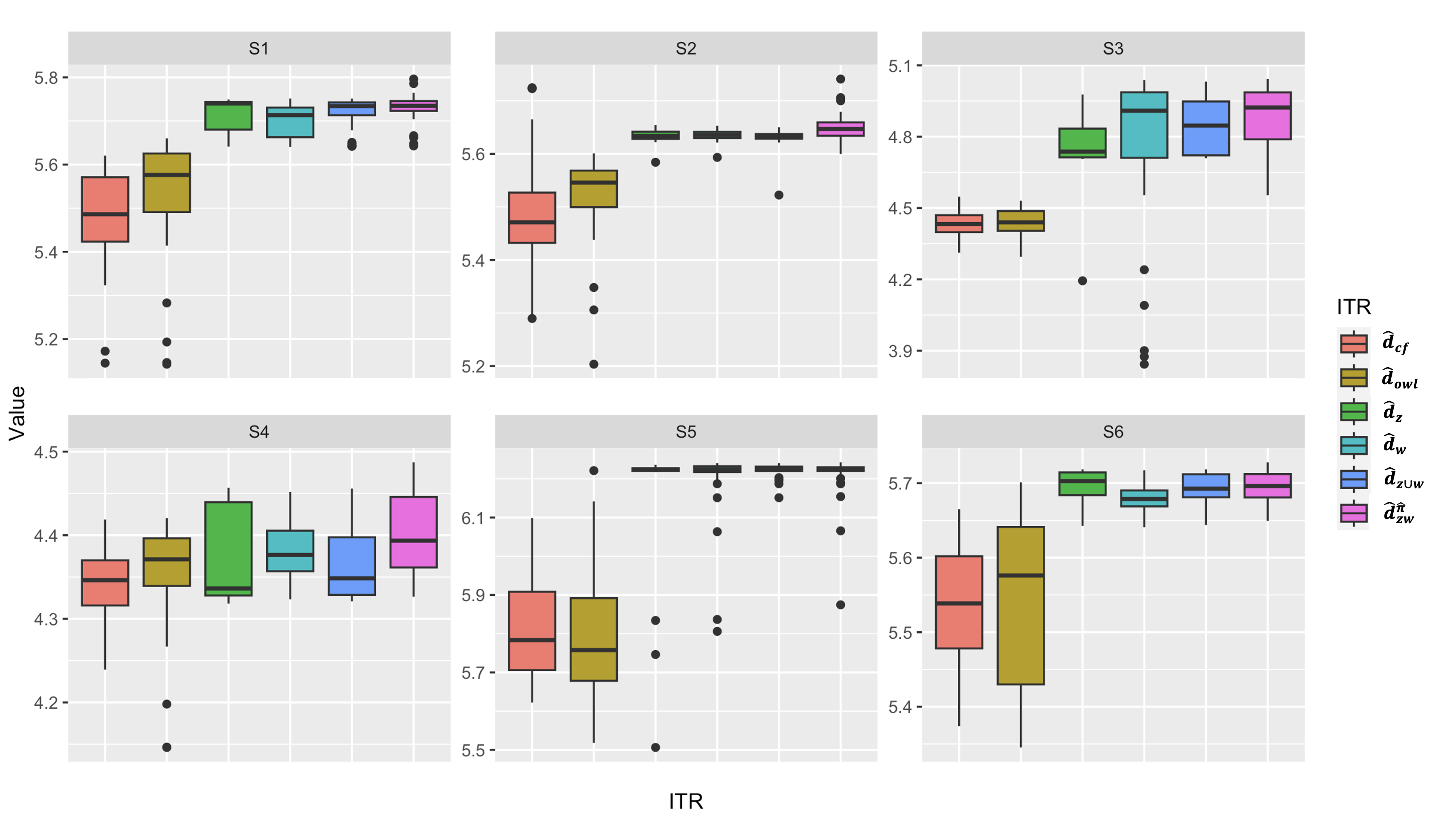
Refer to caption
Figure 4: Boxplots of the empirical value functions with n=500n=500.
Refer to caption
Figure 5: Boxplots of the empirical value functions with n=500n=500 and an altered behavior policy.

Appendix M Additional results of real data application

Regarding the quantitative analysis, Table 4 describes the estimated value functions of our proposed ITR, alongside existing approaches, under four settings with increasing numbers of proxies. For Setting 1, Z=(p​a​f​i​1,p​a​c​o​21)Z=(pafi1,paco21), W=(p​h​1,h​e​m​a​1)W=(ph1,hema1). For Setting 2, Z=(p​a​f​i​1,p​a​c​o​21,p​o​t​1)Z=(pafi1,paco21,pot1), W=(p​h​1,h​e​m​a​1,b​i​l​i​1)W=(ph1,hema1,bili1). For Setting 3, Z=(p​a​f​i​1,p​a​c​o​21,p​o​t​1,w​t​0)Z=(pafi1,paco21,pot1,wt0), W=(p​h​1,h​e​m​a​1,b​i​l​i​1,s​o​d​1)W=(ph1,hema1,bili1,sod1). For Setting 4, Z=(p​a​f​i​1,p​a​c​o​21,p​o​t​1,w​t​0,c​r​e​a​1)Z=(pafi1,paco21,pot1,wt0,crea1), W=(p​h​1,h​e​m​a​1,b​i​l​i​1,s​o​d​1,a​l​b​1)W=(ph1,hema1,bili1,sod1,alb1).

V^​(d^c​f)\hat{V}(\hat{d}_{cf}) V^​(d^o​w​l)\hat{V}(\hat{d}_{owl}) V^​(d^z)\hat{V}(\hat{d}_{z}) V^​(d^w)\hat{V}(\hat{d}_{w}) V^​(d^z∪w)\hat{V}(\hat{d}_{z\cup w}) V^​(d^z​wπ^)\hat{V}(\hat{d}_{zw}^{\hat{\pi}})
Setting 1 24.84 (3.06) 24.97 (2.93) 25.12 (4.69) 26.61 (3.34) 27.86 (2.28) 28.21 (3.28)
Setting 2 24.81 (3.11) 24.97 (2.94) 25.60 (3.73) 25.74 (3.57) 26.32 (2.29) 27.02 (2.95)
Setting 3 24.79 (3.02) 24.97 (2.93) 26.12 (3.61) 25.53 (3.29) 26.76 (2.76) 27.83 (3.03)
Setting 4 24.90 (3.18) 24.97 (2.93) 25.26 (4.76) 25.81 (3.03) 27.38 (2.74) 27.96 (3.07)
Table 4: Estimated values for different ITRs under different proxy variable settings.

As for the qualitative analysis, we present an illustrative example below. Regarding the estimated ITRs in Setting 1, the coefficient of c​a​t​1​_​l​u​n​gcat1\_lung is negative with a minor magnitude for d^z\hat{d}_{z}, contrasting with a positive and relatively large coefficient observed for d^w\hat{d}_{w}, which mirror the outcomes outlined in Qi et al. 2023. This finding suggests that, within the primary disease category of patients with lung cancer, d^z\hat{d}_{z} advocates for undergoing RHC, while d^w\hat{d}_{w} displays a notably inconclusive trend. As evidenced by π^\hat{\pi}, the prevailing trajectory for patients with c​a​t​1​_​l​u​n​g=1cat1\_lung=1 involves a strong inclination toward undergoing RHC, i.e., π^​(X)=1\hat{\pi}(X)=1, aligning with the guidance offered by d^z\hat{d}_{z}. Significantly, the domain knowledge underscores the potential for patients with advanced lung cancer to develop complications like pulmonary hypertension and coma, potentially warranting RHC for assessing pulmonary vascular changes and informing treatment strategies [Galie et al. 2009], which lends support to the recommendations offered by our proposed regime. Furthermore, it is important to note that the whole group of patients can be regarded as unions of multiple subgroups based on various distinct features, and the superiority of d^w\hat{d}_{w} is evident in some subgroups (e.g., a​m​i​h​xamihx). These results show that our proposed ITR offers superior efficacy compared to d^z,d^w\hat{d}_{z},\hat{d}_{w} and d^z∪w\hat{d}_{z\cup w} as our methodology incorporates selection through π^\hat{\pi}.