bimj.200100000 \VolumeXX \IssueXX \Year2021 \pagespan1
zzz \Reviseddatezzz \Accepteddatezzz
Measuring covariate balance in weighted propensity score analyses by the weighted z-difference
Abstract
Propensity score (PS) methods have been increasingly used in recent years when assessing treatment effects in nonrandomized studies. In terms of statistical methods, a number of new PS weighting methods were developed, and it was shown that they can outperform PS matching in efficiency of treatment effect estimation in different simulation settings. For assessing balance of covariates in treatment groups, PS weighting methods commonly use the weighted standardized difference, despite some deficiencies of this measure like, for example, the distribution of the weighted standardized difference depending on the sample size and on the distribution of weights. We introduce the weighted z-difference as a balance measure in PS weighting analyses and demonstrate its usage in a simulation study and by applying it to an example from cardiac surgery. The weighted z-difference is computationally simple and can be calculated for continuous, binary, ordinal and nominal covariates. By using Q-Q-plots we can compare the balance of PS weighted samples immediately to the balance in perfectly matched PS samples and to the expected balance in a randomized trial.
keywords
Propensity score; Standardized difference; Weighted z-difference; Z-difference;1 Introduction
Propensity score (PS) methods are widely used to control for confounding in nonrandomized trials, and have several epistemological as well as statistical advantages as compared to standard regression modelling (Kuss et al. 2016). In essence, propensity score modelling consists of a two-step procedure. In a first step, the individual propensity score, the probability of being treated given the covariates, is estimated, usually by logistic regression. In the second step, the treatment effect is estimated preferably by using either weighting for the PS or matching on the PS (Austin 2011; Austin 2009a). When using PS weighting, inverse probability treatment weights (IPTW, Robins et al. 2000) are generally used, but also several new methods, e.g., matching weights (Li and Greene 2013) or overlap weights (Li et al. 2015) have been developed.
An important part of each PS analysis is to assess balance of covariates between treatment groups in the analysis sample (Harder et al. 2010). To this task, a number of statistical measures has been introduced (Belitser et al. 2011; Franklin et al. 2014), of which the standardized difference (Austin 2009b) is used most widely. For matched PS analysis, Kuss 2013 has advanced the idea of Hill et al. 2000 and Senn 1994 and proposed the z-difference as a balance measure. The z-difference measures balance on a scale that is standard Gaussian under the null hypothesis of balance, that is, if there is no difference in baseline distributions between treatment and control group. As compared to the standardized difference, the z-difference has the two main advantages that its distribution does not depend on sample size and it allows comparing balance of baseline covariates on all scales, that is, for continuous, binary, ordinal, or nominal covariates (Kuss 2013). In PS matching, the z-difference has been successfully used in applied research by us (Furukawa et al. 2017; Furukawa et al. 2018) and others (Fischer et al. 2017; Robinski et al. 2017; Mennander et al. 2020).
However, the z-difference cannot be used with PS weighting, because it can not deal with the individual PS weights that are attached to each observation, but it would be certainly useful to have balance measures also for weighted PS analyses. Austin 2008a proposed a weighted standardized difference to this task, but this inherits the disadvantages of the unweighted standardized difference. That is, it is only defined for continuous and binary variables, and, as we will show later, its distribution also depends on the sample size. Moreover, and as an additional disadvantage, the distribution of the weighted standardized difference depends on the distribution of the weights themselves, which additionally impedes its interpretation.
In this article, we propose a weighted z-difference that does not have these disadvantages and can be used to assess covariate balance in weighted PS analyses while inheriting the advantages of the original z-difference. In section 2 we re-iterate the unweighted z-difference and explain the difference to the unweighted standardized difference. In section 3 the weighted z-difference is introduced for the four different possible scales of covariates, that is, continuous, binary, ordinal and nominal. Section 4 gives results from simulations that demonstrate the advantages of the weighted z-difference in comparison to the weighted standardized difference. In section 5 the weighted z-difference is applied to a published PS matching analysis using IPTW and matching weights. We finish with a discussion of our findings in section 6.
2 The z-difference and the standardized difference
For notation, we assume that a data set with observations and covariates is available, where we aim for these covariates to be balanced in our PS analysis. In addition, a binary treatment variable, whose effect estimate is our primary interest, is given. Before final effect estimation, the balance of covariates in the two treatment groups should be assessed, and the z-difference as well as the standardized difference have been proposed to this task.
For re-iterating the idea of the original z-difference we consider a single covariate, where we denote the observations from the treatment group as and the observations from the control group as . Throughout the paper we will make the assumption that the variables and are independently and identically distributed with potentially different distributions in the two groups. Expected values and variances of the two distributions are denoted by EVar, and Var. We estimate by and by , and analogously for and .
The basic idea of the original z-difference was to measure covariate balance by a statistic that is asymptotically standard Gaussian distributed under the null hypothesis that some properties of the two distributions of and are equal. For example, in the case of a continuous covariate the null hypothesis might be that , or , or both. To be concrete, to test the null hypothesis we previously used the mean difference to measure distance of means between groups. By dividing the mean difference by its standard deviation we achieve the z-difference
| (1) |
and as a consequence of the central limit theorem this z-difference is asymptotically standard Gaussian distributed under the null hypothesis.
Opposed to the z-difference the standardized difference for continuous covariates is defined by Austin 2009b
| (2) |
If we additionally assume then we can replace and by a pooled variance estimator and the formulas of the z-difference and standardized difference simplify to
| (3) |
and
| (4) |
Comparing z-difference and standardized difference we find . Remembering that the z-difference is distributed under the null hypothesis, it follows that the standardized difference is distributed (Austin and Stuart 2015) and thus depends on the sample size.
3 The weighted z-difference
In weighted PS analyses, each single observation comes with a PS weight , that is, an additional multiplicative factor. For computational reasons we assume that the weights in each group are scaled, that is, . As the original standard z-difference was only defined for matched PS analysis where no weights are given, we introduce the weighted z-difference in the following. It will be seen that the weighted z-difference generalizes the z-difference, where the z-difference results when and . All weighted z-differences are implemented in the R package weightedZdiff (Filla 2020), which is available on the Comprehensive R Archive Network (CRAN).
3.1 The continuous case: Comparing means
For continuous covariates we propose to compare the expected mean values in the weighted sample by their difference to check the null hypothesis . The expected value in a weighted sample is estimated by , and analogously for . Calculation of the standard deviation for the weighted mean difference is straightforward using the independence assumption for the variables and . We obtain
| (5) |
and the analogous result for Var.
Finally by using the weighted variance estimator (Austin and Stuart 2015)
| (6) |
for , and analogously for , the weighted z-difference for comparing means of continuous covariates is defined by
| (7) |
The standard Gaussian distribution of under the null hypothesis of balance follows from the central limit theorem for weighted observations of Lindeberg (Chow and Teicher 1978).
The relation of the z-difference and the standardized difference carries over to the weighted case. Under the assumption of equal variances we can use a pooled variance estimator and the formula of reduces to
| (8) |
In parallel, the weighted standardized difference is given by
| (9) |
and we find the ratio .
As is standard Gaussian distributed, follows a distribution. That is, the distribution of the weighted standardized difference additionally depends on the distribution of the weights. In chapter 4 we will show how this complicates checking covariate balance using the weighted standardized difference.
3.2 The continuous case: Comparing variances
Continuous covariates can not only be different with respect to their means, but also with respect to higher moments (Austin 2008b; Rubin 2001). Thus we also propose a weighted z-difference using the difference of weighted variances for assessing balance, which tests the null hypothesis . For computational simplicity we go over to the centered variables and , whereby and are replaced by their weighted estimators and . Centering changes the variance estimator in (6) to
| (10) |
The variance of is given by
Finally, if we let be the weighted variance estimator of Var, then the weighted z-difference for the variances of a continuous variable is given by
| (11) |
Analogous to the case of means for continuous variables, the standard Gaussian distribution for follows from the central limit theorem for weighted observations and the null hypothesis .
3.3 The binary case
For binary covariates we use the difference of the weighted outcome prevalences and as the balance measure. The respective estimate of in the weighted sample is , and analogously for .
Calculation of the variance of is straightforward due to the independence assumption of and and we find
| (12) |
and analogously for Var.
Finally we end up with the weighted z-difference for binary covariates
| (13) |
Again, the standard Gaussian distribution for follows from the central limit theorem for weighted observations and the null hypothesis .
3.4 The ordinal case
For ordinal covariates, the z-difference has to respect the order of observations and we therefore use the expected mean rank difference for ranks . It is important to note that ranking is performed only with respect to the observations itself, but independent of the weights. We estimate the expected mean rank in the weighted sample by and .
The variance of the estimated weighted rank difference is given by
| (14) |
Under the null hypothesis of identically distributed variables and we have , , and .
This yields
Finally we replace and by their estimators and and the weighted z-difference for ordinal covariates is defined by
| (15) |
The standard Gaussian distribution of follows from the central limit theorem for weighted observations together with the theorem of Hájek 1968 which assures that a linear function of the ranks converges to a Gaussian distribution.
3.5 The nominal case
The derivation of the weighted z-difference for a nominal covariate relies on the idea of Gagunashvili 2006 to compare two histograms of weighted observations. We consider a nominal covariate with different categories () with probabilities and of belonging to category of the treatment or control group. We estimate by and analogously for , where denotes the indicator function. Gagunashvili gave an estimator of the variance of by , which is just the sum of squared weights for each cell of the underlying table. Estimating all , and comparing observed and expected probabilities yields
| (16) |
Gagunashvili showed that is -distributed with degrees of freedom under the null hypothesis of for all . We note that the Gagunashvili statistic closely resembles the standard weighted -statistic that we would expect here. Indeed, the numerator of the Gagunashvili statistic and the standard weighted statistic are identical, however, in the denominator, Gagunashvili additionally accounts for the variability of weights.
As the z-difference for nominal covariates should also be standard Gaussian distributed, we apply a probability integral transformation (Deng 1998) to and finally arrive at
| (17) |
with being the cumulative distribution function of a distribution with degrees of freedom and the inverse cumulative distribution function (or quantile) function of the standard normal distribution.
4 Simulation study
To assess the statistical properties of the weighted z-difference in finite samples, we performed three simulation experiments. First we varied the sample sizes, second we used different methods for generating the weights and lastly we changed the ratio of sample sizes in treatment versus control group. In each experiment we compared the weighted z-difference to the weighted standardized difference, the current standard for assessing covariate balance in weighted PS analyses.
4.1 Continuous covariate, varying sample sizes, uniform weights
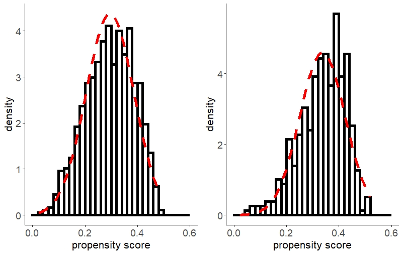
We varied sample sizes between and with a step size of and generated data sets for each single sample size. Theis sample size range was informed by a random sample of 50 PS analyses, published in 2018, from the PUBMED database. For each dataset, we generated standard normally distributed observations, and randomly split the observations in control and treatment groups. This simulation algorithm generates observations, that is, balanced observations in both groups. Each observation was assigned a random weight, which we wanted to generate as realistic as possible. To this task, we used the observed propensity scores from the example data set, which is described in detail in the next section. We fitted Gaussian distributions through the observed propensity scores in treatment and control group (see figure 1) and achieved means of and and a identical standard deviation of . The propensity scores used in the simulation were then sampled from these distributions, whereby we set values smaller than or larger than to and respectively. The samples propensity scores were then transformed to yield the respective weights. In the first setting we used matching weights to create rather similar weights with a small variability.
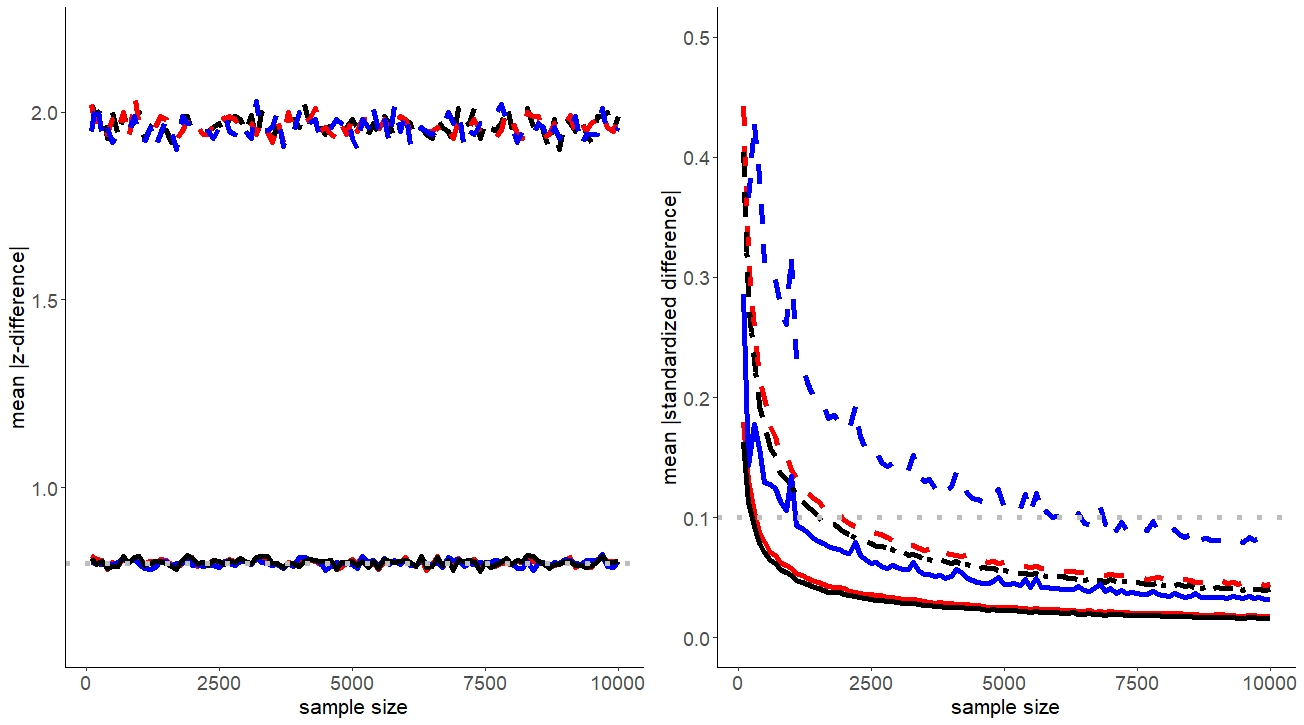
In figure 2 we give mean absolute values for the weighted z-difference and the weighted standardized difference, respectively, across the different sample sizes. The value of the weighted standardized difference depends on the respective sample size with values considerably above for smaller sample sizes. Actually, weighted standardized differences below are in generally considered to indicate good balance (Normand et al. 2001). However, with small sample sizes, even good balance gives considerably larger values of the weighted standardized difference and the rule-of-thumb of using as a cut-off for good balance is too strict here.
Compared to this the weighted z-difference scatters narrowly for the complete range of sample sizes around the value of . This is the value that we expect for the absolute value of a standard Gaussian distributed random variable (Geary 1935).

4.2 Continuous covariate, varying sample sizes, different distribution of weights
In the second simulation we changed the setting from the first simulation by two aspects. First, we used three different weighting schemes, which were (i) constant () weights, (ii) matching weights as in the previous simulation, and (iii) IPTW weights. Second, we increased the variability of the weights by doubling the variance of the distribution used for propensity score generation. Because it is well known that IPTW weights have increased variability as compared to other weighting methods, in this second simulation we are able to assess the difference between the weighted standardized difference and weighted z-difference for weights with (i) no variability, (ii) small variability and (iii) large variability. In figure 3 we give the respective results. It is obvious that the distribution of the weighted standardized difference depends on the weights distribution, e.g., for a small sample size of observations for each group, we observe a mean value of for constant weights, for matching weights, and above for IPTW weights. This is again in conflict with the rule-of-thumb of using the value of to separate good vs. bad covariate balance. Opposed to this, the weighted z-difference does not depend on the distribution of weights and scatters again around its expected value of .
4.3 Binary covariate, varying ratio of observations in treatment vs. control group
In the third simulation we simulated the behaviour of the weighted z-difference and the weighted standardized difference by changing the ratio of sample size in control and treatment group. We chose the case of a binary covariate and varied the percentage of observations in the control group from to . We kept the overall sample size constant at for each single percentage to have at least observations in each group. For generating weights we used the Gaussian distributions and matching weights as described for the first simulation setting.
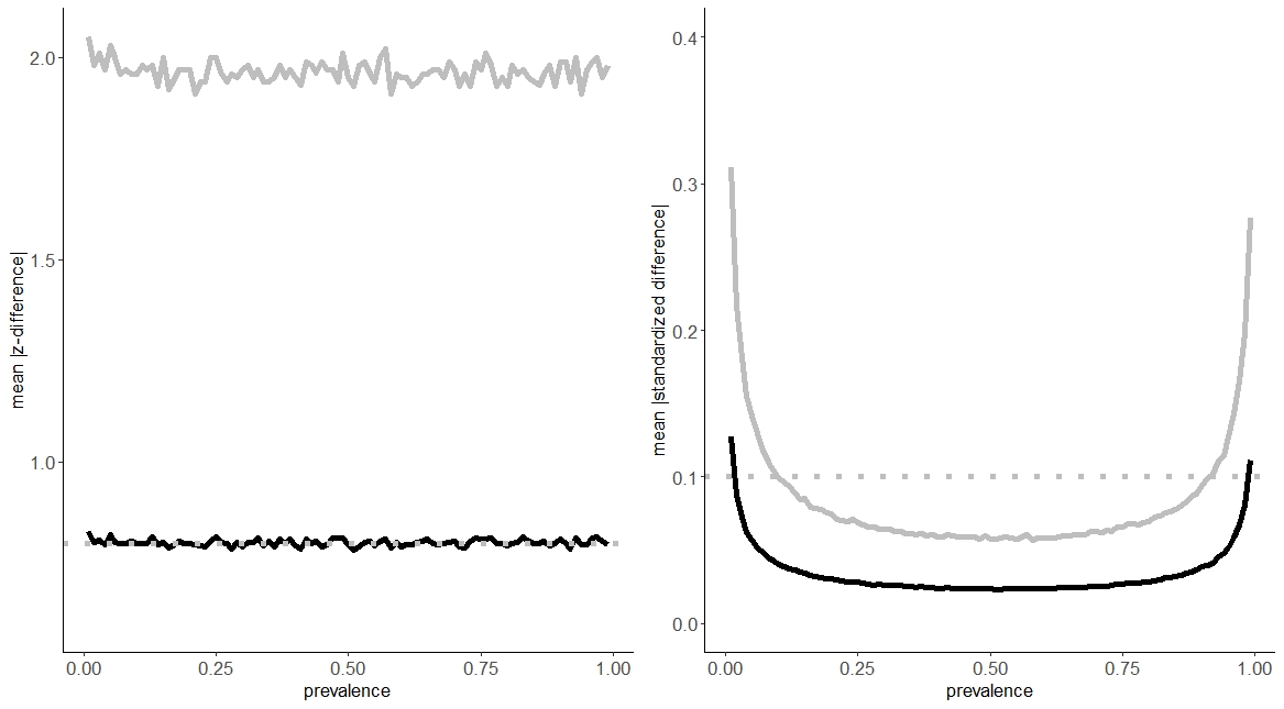
In figure 4 we can see that the mean value of the absolute weighted standardized difference is changing with the different ratios. In fact we observe mean absolute values if the sample size in one group is extremely smaller than in the other (above ) and values in the range between and . In figure 4, it can be seen that the weighted z-difference is not affected by the group size ratio.
As a conclusion from the three simulation experiments we find that the weighted standardized difference will only be of help for assessing balance when sample size, weights distribution, and the ratio of numbers in treatment and control group are simultaneously taken into consideration. This is not the case for the weighted z-difference which can be used to measure covariate balance independent from these three factors.
5 An applied example
In this chapter we apply weighted z-differences to data of a published PS analysis in coronary bypass surgery (Börgermann et al. 2012). The data set contains survival data of patients that received either conventional coronary artery bypass grafting ( or a clampless off-pump coronary artery bypass () for the treatment of coronary artery disease. All operations were performed at the Herz- und Diabeteszentrum NRW, Bad Oeynhausen, Germany, between July and November and the decision, which operation was conducted was made by the patient’s surgeon. The covariates in table 1 were used to estimate the propensity score by standard logistic regression and to derive IPTW as well as matching weights (Li and Greene 2013). Covariate balance was assessed by using the weighted z-differences in the three differentially weighted samples where all weights in the original, unweighted data were set to one. Additionally we also give means and standard deviation for the continuous covariates and relative frequencies for binary, ordinal and nominal covariates in the weighted samples. As the original data set does not contain a nominal covariate, we randomly split the ”yes” category of the covariate variable ”main stem stenosis” in two new categories resulting in a now three-valued nominal covariate. In the unweighted sample, the weighted z-differences reproduce, as expected, the standard z-differences from the data set before PS-matching as given in our previous publication (Kuss 2013). We observe considerable imbalance for age (), Diabetes (), Priority () and the variance of LVEF (), keeping in mind that an absolute value of more than would indicate statistically significant deviations from the balance that would be achieved by randomization.

| Unweighted | Matching weights | Inverse probability weighting | |||||||
| Covariates | cCABG | Clampless OPCAB | Z-difference | cCABG | Clampless OPCAB | Z-difference | cCABG | Clampless OPCAB | Z-difference |
| Continuous scale (based on the difference of means) | |||||||||
| Age (years) | 67.51 (9.44) | 69.31 (9.09) | -3.24 | 69.15 (8.88) | 69.31 (9.09) | -0.35 | 68.00 (9.29) | 67.15 (10.11) | 1.38 |
| BMI (kg/m2) | 28.27 (4.47) | 27.80 (4.21) | 1.83 | 27.87 (4.14) | 27.80 (4.21) | 0.29 | 28.16 (4.37) | 28.31 (4.51) | -0.53 |
| LVEF (%) | 55.39 (14.06) | 56.66 (12.25) | -1.64 | 56.67 (13.47) | 56.66 (12.25) | 0.04 | 55.77 (13.90) | 56.04 (12.37) | -0.31 |
| Previous surgeries (n) | 0.08 (0.39) | 0.05 (0.26) | 1.56 | 0.05 (0.26) | 0.05 (0.26) | 0.17 | 0.07 (0.35) | 0.09 (0.38) | -1.3 |
| Binary scale | |||||||||
| Gender (% female) | 22.1 | 21.77 | 0.13 | 21.52 | 21.80 | -0.11 | 21.93 | 22.1 | -0.06 |
| Hypertension (%) | 84.1 | 82.28 | 0.8 | 82.85 | 82.45 | 0.17 | 83.69 | 84.71 | -0.4 |
| Diabetes (%) | 31.68 | 22.78 | 3.39 | 23.01 | 22.93 | 0.03 | 29 | 28.5 | 0.17 |
| COPD (%) | 7.1 | 5.82 | 0.88 | 5.64 | 5.85 | -0.13 | 6.65 | 5.99 | 0.41 |
| Renal insufficiency (%) | 1.24 | 0.76 | 0.84 | 0.82 | 0.76 | 0.1 | 1.11 | 1.02 | 0.15 |
| Previous MI (%) | 35.74 | 27.09 | 3.14 | 27.36 | 27.26 | 0.03 | 33.14 | 35.29 | -0.71 |
| Previous stroke (%) | 2.37 | 1.01 | 1.89 | 1.07 | 1.02 | 0.07 | 1.96 | 1.85 | 0.11 |
| PAD (%) | 11.39 | 11.9 | -0.26 | 11.47 | 11.74 | -0.13 | 11.4 | 10.83 | -0.27 |
| Preoperative IABP (%) | 1.47 | 1.01 | 0.7 | 1.07 | 1.02 | 0.08 | 1.34 | 1.4 | -0.08 |
| Ordinal scale | |||||||||
| Priority (%) | 4.82 | -0.88 | -0.38 | ||||||
| Elective | 80.95 | 91.90 | 89.39 | 91.85 | 83.55 | 83.53 | |||
| Urgent | 9.81 | 2.53 | 6.58 | 2.55 | 8.81 | 2.89 | |||
| Emergent | 8.68 | 5.32 | 3.81 | 5.35 | 7.18 | 13.04 | |||
| Ultima ratio | 0.56 | 0.25 | 0.22 | 0.25 | 0.46 | 0.54 | |||
| Nominal scale | |||||||||
| Main stem stenosis (%) | -3.53 | -0.03 | 0.11 | ||||||
| Yes | 25.32 | 25.48 | 25.46 | 25.54 | 24.73 | 25.47 | |||
| No | 33.16 | 23 | 32.76 | 32.12 | 25.22 | 25.87 | |||
| Unclear | 41.52 | 51.52 | 41.78 | 42.34 | 50.05 | 48.66 | |||
| Continuous scale (based on the difference of variances) | |||||||||
| Age (years) | 67.51 (9.44) | 69.31 (9.09) | 0.9 | 69.06 (8.82) | 69.26 (9.09) | -0.65 | 68.00 (9.29) | 67.15 (10.11) | -2.02 |
| BMI (kg/m2) | 28.27 (4.47) | 27.80 (4.21) | 1.08 | 27.90 (4.14) | 27.82 (4.21) | -0.27 | 28.16 (4.37) | 28.31 (4.51) | -0.54 |
| LVEF | 55.39 (14.06) | 56.66 (12.25) | 2.8 | 56.62 (13.52) | 56.66 (12.25) | 1.83 | 55.77 (13.90) | 56.04 (12.37) | 2.13 |
| Previous surgeries (n) | 0.08 (0.39) | 0.05 (0.26) | 1.09 | 0.05 (0.26) | 0.05 (0.26) | 0.02 | 0.07 (0.35) | 0.09 (0.38) | -0.28 |
Covariate balance is largely improved in the weighted samples after applying IPTW and matching weights, where the matching weights method outperforms the standard IPTW method: the mean absolute value of the weighted z-differences is (variance ) for equal weights, () for IPTW, and () for matching weights. The different performances in covariate balancing can also be seen from the Q-Q-plot for the weighted z-differences in figure 5. From such a plot we would expect to see (unweighted) z-differences from a randomized trial to lie on a line through the origin with a unit slope (Kuss 2013). In addition, unweighted and weighted z-differences could also be compared to a perfectly matched PS analysis in the sense of Rubin and Thomas 1992; Rubin and Thomas 1996 from which we would expect the values to lie on a line through the origin with slope . The raw unweighted z-differences clearly deviate from the line with slope , indicating systematic differences between the original treatment groups. However, for both weighting methods the slope of the weighted quantiles is smaller than , pointing to an even better balance in the weighted samples as compared to a perfectly matched sample.
6 Discussion
In this paper, we propose weighted z-differences to measure covariate balance in weighted propensity score analyses. In comparison to the weighted standardized difference of Austin, we see three advantages of weighted z-differences. First, weighted z-differences can be used for continuous, binary, ordinal and nominal covariates, and not just for continuous and binary ones. Second, the distribution of the weighted z-difference is independent of the sample size, which allows comparison of data sets of different sizes. Third, the distribution of the weighted z-difference is, again in contrast to the weighted standardized difference, independent of the distribution of the weights. Weighted z-differences are straightforward generalizations of our previous proposal of z-differences in matched PS analyses and, at least in the continuous and the binary covariate case, reduce to standard z-differences in the unweighted case. The idea of the double transformation from a to a standard normal distribution in the nominal covariate case now also allows for a standard, unweighted z-difference. Finally, weighted z-differences can be used for all types of weights (e.g., standard IPTW weights (Horvitz and Thompson 1952), but also matching (Li and Greene 2013), optimal (Li et al. 2015), or ATT/ATC weights (Li et al. 2015)), and thus not only allow optimizing and comparing covariate balance with respect to the covariates included, but also with respect to the respective weight type. Due to the ”z-property” of weighted and unweighted z-differences, covariate balance can also be compared (e.g., by using the sum of z-differences across all covariates) between a weighted PS analyses and PS-matching. As such, also the previously proposed Q-Q-plots to compare covariate balance 1) across PS methods, 2) to the expected balance in a randomized trial, and 3) to a perfectly PS matched data set in the sense of Rubin and Thomas can be used. We also emphasize that the z-difference is a global balance measure that can also be used outside of propensity score methods, e.g. in randomized trials, to measure the balance of observations in two groups.
It is fair to point to some limitations of weighted z-differences. We observed the weighted z-difference for nominal covariates to be somewhat sensitive against very low numbers of observations in some categories of the covariate, and Gagunashvili recommended to have at least ten observations within each cell (Gagunashvili 2006). In the case of very sparse data, we propose as a solution to calculate weighted binary z-differences for each dichotomization of the nominal covariate against a reference category. Another limitation of the weighted z-difference in the PS setting is that it can be only applied with PS-weighting methods. In contrast, Austin 2009c showed, how weighted standardized differences can also be used when stratifying on or adjusting for the propensity score.
Balancing advantages and limitations we recommend weighted z-differences for assessing covariate balance in weighted PS analyses.
Conflict of Interest
The authors have declared no conflict of interest. (or please state any conflicts of interest)
References
- Kuss et al. (2016) Kuss, O., Blettner, M. and Börgermann, J. 2016. Propensity Score: an Alternative Method of Analyzing Treatment Effects. Deutsches Ärzteblatt International 113, 597–603.
- Austin (2011) Austin, P.C. 2011. An Introduction to Propensity Score Methods for Reducing the Effects of Confounding in Observational Studies. Multivariate Behavioral Research 46, 399–424.
- Austin (2009a) Austin, P.C. 2009a. The relative ability of different propensity score methods to balance measured covariates between treated and untreated subjects in observational studies. Medical Decision Making 29, 661–677.
- Robins et al. (2000) Robins, J.M., Hernán, M.A. and Brumback, B. 2000. Marginal structural models and causal inference in epidemiology. Epidemiology 11, 550–560.
- Li and Greene (2013) Li, L. and Greene, T. 2013. A weighting analogue to pair matching in propensity score analysis. International Journal of Biostatistics 9, 215–234.
- Li et al. (2015) Li, F., Morgan, K.L. and Zaslavsky, A.M. 2018. Balancing covariates via propensity score weighting. Journal of the American Statistical Association 113, 390–400.
- Harder et al. (2010) Harder, V.S., Stuart, E.A. and Anthony, J.C. 2010. Propensity score techniques and the assessment of measured covariate balance to test causal associations in psychological research. Psychological Methods 15, 234–249.
- Belitser et al. (2011) Belitser, S.V., Martens, E.P., Pestman, W.R., Groenwold, R.H., de Boer, A. and Klungel, O.H. 2011. Measuring balance and model selection in propensity score methods. Pharmacoepidemiology and Drug Safety 20, 1115–1129.
- Franklin et al. (2014) Franklin, J.M., Rassen, J.A., Ackermann, D., Bartels, D.B. and Schneeweiss, S. 2014. Metrics for covariate balance in cohort studies of causal effects. Statistics in Medicine 33, 1685–1699.
- Austin (2009b) Austin, P.C. 2009b. Using the standardized difference to compare the prevalence of a binary variable between two groups in observational research. Communications in Statistics - Simulation and Computation 38, 1228–1234.
- Kuss (2013) Kuss, O. 2013. The z-difference can be used to measure covariate balance in matched propensity score analyses. Journal of Clinical Epidemiology 66, 1302–1307.
- Hill et al. (2000) Hill, J., Rubin, D.B. and Thomas, N. 2000. The Design of the New York School Choice Scholarship Program Evaluation. In: Bickman L. [ed.] Research Design: Donald Campbell’s Legacy. Thousand Oaks: Sage Publications; 2000. 155-180.
- Senn (1994) Senn, S. 1994. Testing for baseline balance in clinical trials. Statistics in Medicine 13, 1715–1726.
- Furukawa et al. (2017) Furukawa, N., Kuss, O., Preindl, K., Renner, A., Aboud, A., Hakim-Meibodi, K., Benzinger, M., Pühler, T., Ensminger, S., Fujita, B., Becker, T., Gummert, J.F. and Börgermann, J. 2017. Anaortic off-pump versus clampless off-pump using the PAS-Port device versus conventional coronary artery bypass grafting: mid-term results from a matched propensity score analysis of 5422 unselected patients. European Journal of Cardio-Thoracic Surgery 52, 760–767.
- Furukawa et al. (2018) Furukawa, N., Kuss, O., Emmel, E., Scholtz, S., Scholtz, W., Fujita, B., Ensminger, S., Gummert, J.F. and Börgermann, J. 2018. Minimally invasive versus transapical versus transfemoral aortic valve implantation: A one-to-one-to-one propensity score-matched analysis. Journal of Thoracic and Cardiovascular Surgery 156, 1825–1834.
- Fischer et al. (2017) Fischer, J., Lupberger, E., Hebsaker, J., Blumenstock, G., Aichinger, E., Yazdi, A.S., Reick, D., Oehme, R. and Biedermann, T. 2017. Prevalence of type I sensitization to alpha-gal in forest service employees and hunters. Allergy 72, 1540–1547.
- Robinski et al. (2017) Robinski, M., Mau, W., Wienke, A. and Girndt, M. 2017. The Choice of Renal Replacement Therapy (CORETH) project: dialysis patients’ psychosocial characteristics and treatment satisfaction. Nephrology Dialysis Transplantation 32, 315–324.
- Mennander et al. (2020) Mennander, A., Olsson, C., Jeppsson, A., Geirsson, A., Hjortdal, V., Hansson, E.C., Jarvela, K., Nozohoor, S., Gunn, J., Ahlsson, A. and Gudbjartsson, T. 2020. The significance of bicuspid aortic valve after surgery for acute type A aortic dissection. Journal of Thoracic and Cardiovascular Surgery 159, 760–767.
- Austin (2008a) Austin, P.C. 2008a. Assessing balance in measured baseline covariates when using many-to-one matching on the propensity-score. Pharmacoepidemiology and Drug Safety 17, 1218–1225.
- Austin and Stuart (2015) Austin, P.C. and Stuart, E.A. 2015. Moving towards best practice when using inverse probability of treatment weighting (IPTW) using the propensity score to estimate causal treatment effects in observational studies. Statistics in Medicine 34, 3661–3679.
- Filla (2020) Filla, T. 2020. WeightedZdiff: Calculation of z-Differences. 2020. Available at: https://CRAN.R-project.org/package=weightedZdiff. Accessed November 5, 2020.
- Chow and Teicher (1978) Chow, Y.S. and Teicher, H. 1978. Probability Theory: Independence, Interchangeability, Martingales. New York: Springer; 1978.
- Austin (2008b) Austin, P.C. 2008b. Primer on statistical interpretation or methods report card on propensity-score matching in the cardiology literature from 2004 to 2006: a systematic review. Circulation: Cardiovascular Quality and Outcomes 1, 62–67.
- Rubin (2001) Rubin, D.B. 2001. Using propensity scores to help design observational studies: application to the tobacco litigation. Health Services and Outcomes Research Methodology 2, 169–188.
- Hájek (1968) Hájek, J. 1968. Asymptotic normality of simple linear rank statistics under alternatives. Annals of Mathematical Statistics 39, 325–346.
- Gagunashvili (2006) Gagunashvili, N. 2006. Comparison of weighted and unweighted histograms. 2006. Available at: https://arxiv.org/abs/physics/0605123. Accessed November 5, 2020.
- Deng (1998) Deng, L.Y. 1998. Uniform distribution. In: Armitage P., Colton T. [eds.] Encyclopedia of Biostatistics. Chichester: John Wiley & Sons; 1998, 4650-4651.
- Normand et al. (2001) Normand, S.T., Landrum, M.B., Guadagnoli, E., Ayanian, J.Z., Ryan, T.J., Cleary, P.D. and McNeil, B.J. 2001. Validating recommendations for coronary angiography following acute myocardial infarction in the elderly: a matched analysis using propensity scores. Journal of Clinical Epidemiology 54, 387–398.
- Geary (1935) Geary, R.C. 1935. The ratio of the mean deviation to the standard deviation as a test of normality. Biometrika 27, 310–332.
- Börgermann et al. (2012) Börgermann, J., Hakim, K., Renner, A., Parsa, A., Aboud, A., Becker, T., Masshoff, M., Zittermann, A., Gummert, J.F. and Kuss, O. 2012. Clampless off-pump versus conventional coronary artery revascularization: a propensity score analysis of 788 patients. Circulation 126, S176–182.
- Rubin and Thomas (1992) Rubin, D.B. and Thomas, N. 1992. Characterizing the Effect of Matching Using Linear Propensity Score Methods with Normal Distributions. Biometrika 79, 797–809.
- Rubin and Thomas (1996) Rubin, D.B. and Thomas, N. 1996. Matching Using Estimated Propensity Scores: Relating Theory to Practice Biometrics 52, 249–264.
- Horvitz and Thompson (1952) Horvitz, D.G. and Thompson, D.J. 1952. A Generalization of Sampling Without Replacement from a Finite Universe. Journal of the American Statistical Association 47, 663–685.
- Austin (2009c) Austin, P.C. 2009c. The relative ability of different propensity score methods to balance measured covariates between treated and untreated subjects in observational studies. Medical Decision Making 29, 661–677.