跳到论文正文
W Papers独立论文阅读器 arXiv:2212.09369 论文正文 计算阅读时间 · 0%
引用这篇论文根据当前论文元数据生成,正式投稿前建议核对。


License: arXiv.org perpetual non-exclusive license
arXiv:2212.09369v1 [math.NA] 19 Dec 2022

Imaging an acoustic obstacle and its excitation sources from phaseless near-field data

Deyue Zhang Thanks: School of Mathematics, Jilin University, Changchun, China, dyzhang@jlu.edu.cn    Yue Wu Thanks: School of Mathematics, Jilin University, Changchun, China, wuy20@mails.jlu.edu.cn       Yukun Guo Thanks: School of Mathematics, Harbin Institute of Technology, Harbin, China. ykguo@hit.edu.cn (Corresponding author)
Abstract

This paper is concerned with reconstructing an acoustic obstacle and its excitation sources from the phaseless near-field measurements. By supplementing some artificial sources to the inverse scattering system, this co-inversion problem can be decoupled into two inverse problems: an inverse obstacle scattering problem and an inverse source problem, and the corresponding uniqueness can be established. This novel decoupling technique requires some extra data but brings in several salient benefits. First, our method is fast and easy to implement. Second, the boundary condition of the obstacle is not needed. Finally, this approximate decoupling method can be applied to other co-inversion problems, such as determining the medium and its excitation sources. Several numerical examples are presented to demonstrate the feasibility and effectiveness of the proposed method.

Keywords: inverse scattering, inverse source problem, phaseless, uniqueness, direct imaging

1 Introduction

Inverse problems of determining unknown excitations or scattering inclusions by acoustic waves appear in diverse areas of scientific and engineering importance, e.g., nondestructive evaluation, sonar detection, and ultrasonic tomography. In many areas of applied sciences, it is very difficult or extremely expensive to access the phased data of the complex-valued time-harmonic wave field, while the phaseless/modulus data is usually much cheaper to acquire [12, 17, 20]. Hence, reconstruction from phaseless data is both theoretically and practically important and has received considerable attention in the literature in recent years [1, 7, 13, 16, 19, 22, 23, 27]. Recently, there is also a surge of interest in the co-inversion problem of simultaneously recovering the source term and the passive inhomogeneity from the scattering measurements, see, e.g. [3, 4, 9, 14, 15]. However, to our knowledge, the simultaneous reconstruction of source and scatterer from phaseless data has not yet been studied in the existing literature.

In this paper, we investigate a new model of simultaneously reconstructing the point sources and the impenetrable obstacle from phaseless scattering data. This phaseless co-inversion problem suffers from the drastic difficulties of nonlinearity and severe ill-posedness, in particular, the dual unknowns and the loss of phase information substantially obstruct the application of algorithms for phased inverse scattering problems. Meanwhile, it is well acknowledged that a lack of information cannot be remedied by merely the mathematical implementation itself and therefore the incorporation of additional information is indispensable for achieving effective reconstruction. To this end, motivated by the techniques of artificial reference sources/objects for phaseless inverse scattering problems [8, 10, 11, 25, 21, 24], as well as the recent decoupling strategy for the interior co-inversion problem [26], in the current work we propose a novel method for tackling the challenging phaseless co-inversion problem. The basic idea of our method is to decode the source and scatterer components from the scattering system with the help of the additional illuminations due to the so-called reference sources. These artificially appended sources play a significant role in decoupling the co-inversion problem into the usual inverse source subproblem and inverse obstacle scattering subproblems. Then the uniqueness issue on these subproblems could be separately analyzed, namely, the shape of the scatterer together with the boundary condition could be uniquely determined, meanwhile, the unknown source locations can be also uniquely identified. Moreover, the decoupled subproblems can be numerically treated easily by the direct sampling scheme and the reverse time migration method, respectively. The overall algorithm works with the data due to only a single frequency and does not rely on any solver of the forward problem. Since the computational demanding process is not involved, the proposed method can be implemented easily. In addition, neither the number of obstacles nor the boundary conditions are required to be priorly known. In our view, the aforementioned features of our study constitute the noteworthy novelty of this article.

The remaining part of this article is organized as follows. In the next section, we introduce the mathematical formulation of the phaseless co-inversion problem as well as the incorporation of reference sources. In section 3, the theoretical results are provided to justify the unique identifiability of underlying sources and obstacles from the modulus of near-field measurements. In section 4, the phaseless co-inversion problem is decoupled into two subproblems of inverse obstacle scattering and inverse source problem. Then the subproblems are tackled respectively with direct imaging indicators. The indicating behavior for locating the sources is analyzed as well. Numerical experiments are presented in section 5 to confirm the theoretical analysis of our inversion process and illustrate the effectiveness and robustness of our newly proposed phaseless co-inversion algorithm.

2 Problem setting

We begin this section by introducing the phaseless co-inversion problem of an obstacle and its excitation point sources under consideration. Let D⊂ℝ2D\subset\mathbb{R}^{2} be a simply connected bounded domain with C2C^{2} boundary ∂D\partial D. For a generic point z∈ℝ2\D¯z\in\mathbb{R}^{2}\backslash\overline{D}, the incident field uiu^{i} due to the point source located at zz is given by

ui​(x,z)=i4​H0(1)​(k​|x−z|),x∈ℝ2\(D∪{z}),u^{i}(x;z)=\frac{\mathrm{i}}{4}H_{0}^{(1)}(k|x-z|),\quad x\in\mathbb{R}^{2}\backslash(D\cup\{z\}), (1)

where H0(1)H_{0}^{(1)} is the Hankel function of the first kind of order zero, and k>0k>0 is the wavenumber. Then, the forward scattering problem can be stated as follows: given the source point zz and the obstacle DD, find the scattered field us​(x,z)u^{s}(x;z) which satisfies the following boundary value problem (see [6]):

Δ​us+k2​us\displaystyle\Delta u^{s}+k^{2}u^{s} =0inℝ2\D¯,\displaystyle=0\quad\mathrm{in}\ \mathbb{R}^{2}\backslash\overline{D}, (2)
ℬ​u\displaystyle\mathscr{B}u =0on∂D,\displaystyle=0\quad\mathrm{on}\ \partial D, (3)
limr:=|x|→∞r(\displaystyle\lim\limits_{r:=|x|\to\infty}\sqrt{r}\bigg( OPEN∂us∂r−i​k​us)=0,\displaystyle\frac{\partial u^{s}}{\partial r}-\mathrm{i}ku^{s}\bigg)=0, (4)

where u⁡(x,z)=ui​(x,z)+us​(x,z)u(x;z)=u^{i}(x;z)+u^{s}(x;z) denotes the total field and eq. 4 is the Sommerfeld radiation condition. Here ℬ\mathscr{B} in eq. 3 is the boundary operator defined by

ℬ​u={u,for a sound-soft obstacle,∂u∂ν+i​k​λ​u,for an impedance obstacle.\mathscr{B}u=\begin{cases}u,&\text{for a sound-soft obstacle},\\ \dfrac{\partial u}{\partial\nu}+\mathrm{i}k\lambda u,&\text{for an impedance obstacle}.\end{cases} (5)

where ν\nu is the unit outward normal to ∂D\partial D and λ\lambda is a real parameter. This boundary condition eq. 5 covers the Dirichlet/sound-soft boundary condition, the Neumann/sound-hard boundary condition (λ=0\lambda=0), and the impedance boundary condition (λ≠0\lambda\neq 0). It is well known that the forward scattering problem (2)-(4) admits a unique solution us∈Hloc1​(ℝ2\D¯)u^{s}\in H_{\rm loc}^{1}(\mathbb{R}^{2}\backslash\overline{D}) (see, e.g., [6, 18]), and the scattered wave usu^{s} has the following asymptotic behavior

us​(x,z)=ei​k​|x||x|​{u∞​(x^,z)+𝒪⁡(1|x|)},|x|→∞u^{s}(x;z)=\frac{\mathrm{e}^{\mathrm{i}k|x|}}{\sqrt{|x|}}\left\{u^{\infty}(\hat{x};z)+\mathcal{O}\left(\frac{1}{|x|}\right)\right\},\quad|x|\to\infty

uniformly in all observation directions x^=x/|x|∈𝕊1:={x∈ℝ2:|x|=1}\hat{x}=x/|x|\in\mathbb{S}^{1}:=\{x\in\mathbb{R}^{2}:|x|=1\}. The complex-valued analytic function u∞​(x^,z)u^{\infty}(\hat{x};z) defined on the unit circle 𝕊1\mathbb{S}^{1} is called the far field pattern or scattering amplitude (see [6]).

Let zj∈ℝ2\D¯​(j=1,⋯,N)z_{j}\in\mathbb{R}^{2}\backslash\overline{D}\,(j=1,\cdots,N) be mutually distinct source points, P:=∪j=1N{zj}P:=\cup_{j=1}^{N}\{z_{j}\}, Bρ={x∈ℝ2:|x|<ρ}B_{\rho}=\{x\in\mathbb{R}^{2}:|x|<\rho\} and Γρ=∂Bρ\Gamma_{\rho}=\partial B_{\rho}, such that (D¯∪P)⊂Bρ\left(\overline{D}\cup P\right)\subset B_{\rho}. Assume that ΓR=∂BR\Gamma_{R}=\partial B_{R} is the measurement curve with BR={x∈ℝ2:|x|<R}B_{R}=\{x\in\mathbb{R}^{2}:|x|<R\} and R>ρR>\rho. Denote the superposition of wave fields by

w(x;P)=∑j=1Nw(x;zj),zj∈P,j=1,⋯,N,w(x;P)=\sum_{j=1}^{N}w(x;z_{j}),\quad z_{j}\in P,\ j=1,\cdots,N,

with ww in place of ui,us,uu^{i},u^{s},u or u∞u^{\infty}, accordingly. Then, the phaseless co-inversion problem under consideration is to determine the obstacle-source pair (∂D,P)(\partial D,P) from the phaseless measurements {|u⁡(x,P)|:x∈ΓR}\{|u(x;P)|:x\in\Gamma_{R}\}.

To our knowledge, this model inverse problem as well as its uniqueness issue were not studied in the literature. Motivated by the reference point techniques for tackling the phaseless inverse scattering problem, we will consider incorporating artificial point sources into the co-inversion system. Let z1,z2∈ℝ2\(D¯∪P)z_{1},z_{2}\in\mathbb{R}^{2}\backslash(\overline{D}\cup P) be two additional source points and t1,t2∈ℝt_{1},t_{2}\in\mathbb{R}. By the linearity of the direct scattering problem, the total field produced by the incident waves ui​(x,P)+t1​ui​(x,z1)+t2​ui​(x,z2)u^{i}(x;P)+t_{1}u^{i}(x;z_{1})+t_{2}u^{i}(x;z_{2}) is given by

u⁡(x,P,t1​z1,t2​z2):=u⁡(x,P)+t1​u​(x,z1)+t2​u​(x,z2),x∈ℝ2\(D¯∪P∪{z1,z2}),u(x;P,t_{1}z_{1},t_{2}z_{2}):=u(x;P)+t_{1}u(x;z_{1})+t_{2}u(x;z_{2}),\ x\in\mathbb{R}^{2}\backslash(\overline{D}\cup P\cup\{z_{1},z_{2}\}),

To introduce the phaseless co-inversion problem with artificial sources, we also need the following definition of the admissible curve.

Definition 2.1 ([23]).

(Admissible curve) An open curve Γ\Gamma is called an admissible curve with respect to domain Ω\Omega if

  • (i)

    Ω\Omega is simply-connected;

  • (ii)

    ∂Ω\partial\Omega is analytic homeomorphic to 𝕊1\mathbb{S}^{1};

  • (iii)

    k2k^{2} is not a Dirichlet eigenvalue of −Δ-\Delta in Ω\Omega;

  • (iv)

    Γ⊂∂Ω\Gamma\subset\partial\Omega is a one-dimensional analytic manifold with nonvanishing measure.

Now, the phaseless co-inversion problem with artificial sources under consideration can be stated as the following.

Problem 2.1 (Phaseless co-inversion problem).

Let DD be the impenetrable obstacle with boundary condition ℬ\mathscr{B} and PP be a set of distinct source points such that (D∪P)⊂Bρ⊂BR(D\cup P)\subset B_{\rho}\subset B_{R}. Assume that Γ\Gamma is an admissible curve with respect to GG with G⊂BR\Bρ¯G\subset B_{R}\backslash\overline{B_{\rho}}. Given the phaseless near-field data

{|u⁡(x,P)|:x∈ΓR},\displaystyle\{|u(x;P)|:x\in\Gamma_{R}\},
{|u(x;P,tℓz0)|:x∈ΓR,ℓ=1,2},\displaystyle\{|u(x;P,t_{\ell}z_{0})|:x\in\Gamma_{R},\ell=1,2\},
{|u(x;P,tℓz)|:x∈ΓR,z∈Γρ∪Γ,ℓ=1,2},\displaystyle\{|u(x;P,t_{\ell}z)|:x\in\Gamma_{R},z\in\Gamma_{\rho}\cup\Gamma,\ell=1,2\},
{|u(x;P,tℓz0,tℓz)|:x∈ΓR,z∈Γρ∪Γ,ℓ=1,2}\displaystyle\{|u(x;P,t_{\ell}z_{0},t_{\ell}z)|:x\in\Gamma_{R},z\in\Gamma_{\rho}\cup\Gamma,\ell=1,2\}

for a fixed wavenumber kk, a fixed z0∈ℝ2\Bρ¯z_{0}\in\mathbb{R}^{2}\backslash\overline{B_{\rho}} and two positive constants t1,t2t_{1},t_{2} with t1≠t2t_{1}\neq t_{2}, determine the obstacle-source pair (∂D,P)(\partial D,P).

We refer to fig. 1 for an illustration of the geometry setting of 2.1.

ΓR\Gamma_{R}BRB_{R}Γρ\Gamma_{\rho}BρB_{\rho}Γ\GammaGGz0z_{0}DD
Figure 1: An illustration of the phaseless co-inversion problem.

3 Uniqueness

In this section, we present the uniqueness result on 2.1, which shows that the location of the point sources, the location and shape ∂D\partial D, as well as the boundary condition ℬ\mathscr{B} for the obstacle, can be simultaneously and uniquely determined from the modulus of near-fields.

Theorem 3.1.

Let D1D_{1} and D2D_{2} be two obstacles with boundary conditions ℬ1\mathscr{B}_{1} and ℬ2\mathscr{B}_{2}, and P1P_{1} and P2P_{2} be two sets of source points, such that ∪j=12(Dj∪Pj)⊂Bρ⊂BR\cup_{j=1}^{2}(D_{j}\cup P_{j})\subset B_{\rho}\subset B_{R}. Assume that Γ\Gamma is an admissible curve for GG with G⊂BR\Bρ¯G\subset B_{R}\backslash\overline{B_{\rho}}. The scattered field and the total field with respect to Dj∪PjD_{j}\cup P_{j} and Dj∪{z}D_{j}\cup\{z\} are denoted by ujs​(x,Pj)u_{j}^{s}(x;P_{j}), uj​(x,Pj)u_{j}(x;P_{j}), ujs​(x,z)u_{j}^{s}(x;z) and uj​(x,z),j=1,2u_{j}(x;z),j=1,2, respectively. If the near-fields satisfy that

|u1​(x,P1)|\displaystyle|u_{1}(x;P_{1})| =|u2​(x,P2)|,∀x∈ΓR,\displaystyle=|u_{2}(x;P_{2})|,\quad\forall x\in\Gamma_{R}, (6)
|u1​(x,P1,tℓ​z)|\displaystyle|u_{1}(x;P_{1},t_{\ell}z)| =|u2(x;P2,tℓz)|,∀(x,z)∈ΓR×(Γρ∪Γ),ℓ=1,2,\displaystyle=|u_{2}(x;P_{2},t_{\ell}z)|,\quad\forall(x,z)\in\Gamma_{R}\times(\Gamma_{\rho}\cup\Gamma),\ \ell=1,2, (7)
|u1​(x,P1,tℓ​z0)|\displaystyle|u_{1}(x;P_{1},t_{\ell}z_{0})| =|u2(x;P2,tℓz0)|,∀x∈ΓR,ℓ=1,2,\displaystyle=|u_{2}(x;P_{2},t_{\ell}z_{0})|,\quad\forall x\in\Gamma_{R},\ \ell=1,2, (8)
|u1​(x,P1,tℓ​z0,tℓ​z)|\displaystyle|u_{1}(x;P_{1},t_{\ell}z_{0},t_{\ell}z)| =|u2(x;P2,tℓz0,tℓz)|,∀(x,z)∈ΓR×(Γρ∪Γ),ℓ=1,2,\displaystyle=|u_{2}(x;P_{2},t_{\ell}z_{0},t_{\ell}z)|,\quad\forall(x,z)\in\Gamma_{R}\times(\Gamma_{\rho}\cup\Gamma),\ {\ell}=1,2, (9)

for an arbitrarily fixed wavenumber kk, a fixed z0∈ℝ2\Bρ¯z_{0}\in\mathbb{R}^{2}\backslash\overline{B_{\rho}} and two positive constants t1,t2t_{1},t_{2} with t1≠t2t_{1}\neq t_{2}. Then we have D1=D2,ℬ1=ℬ2D_{1}=D_{2},\mathscr{B}_{1}=\mathscr{B}_{2} and P1=P2P_{1}=P_{2}.

Proof.

The proof is divided into two parts.

(i) Uniqueness for the obstacle. From eq. 6 and eq. 7, we have for all x∈ΓR,z∈Γρ∪Γx\in\Gamma_{R},z\in\Gamma_{\rho}\cup\Gamma and ℓ=1,2\ell=1,2,

tℓ​(|u1​(x,z)|2−|u2​(x,z)|2)=2​Re​(u2​(x,P2)​u2​(x,z)¯−u1​(x,P1)​u1​(x,z)¯)t_{\ell}\left(|u_{1}(x;z)|^{2}-|u_{2}(x;z)|^{2}\right)=2\mathrm{Re}\left(u_{2}(x;P_{2})\overline{u_{2}(x;z)}-u_{1}(x;P_{1})\overline{u_{1}(x;z)}\right)

where the overline denotes the complex conjugate. Further, by tℓ>0t_{\ell}>0 (ℓ=1,2)(\ell=1,2) and t1≠t2t_{1}\neq t_{2}, we obtain

|u1​(x,z)|\displaystyle|u_{1}(x;z)| =|u2​(x,z)|,∀(x,z)∈ΓR×(Γρ∪Γ),\displaystyle=|u_{2}(x;z)|,\quad\forall(x,z)\in\Gamma_{R}\times(\Gamma_{\rho}\cup\Gamma), (10)
Re⁡(u1​(x,P1)​u1​(x,z)¯)\displaystyle\mathrm{Re}\left(u_{1}(x;P_{1})\overline{u_{1}(x;z)}\right) =Re⁡(u2​(x,P2)​u2​(x,z)¯),∀(x,z)∈ΓR×(Γρ∪Γ).\displaystyle=\mathrm{Re}\left(u_{2}(x;P_{2})\overline{u_{2}(x;z)}\right),\ \forall(x,z)\in\Gamma_{R}\times(\Gamma_{\rho}\cup\Gamma). (11)

Similarly, from eq. 6, eq. 8 and eq. 9, we deduce that

|u1​(x,z0)|\displaystyle|u_{1}(x;z_{0})| =|u2​(x,z0)|,∀x∈ΓR,\displaystyle=|u_{2}(x;z_{0})|,\quad\forall x\in\Gamma_{R}, (12)
|u1​(x,z,z0)|\displaystyle|u_{1}(x;z,z_{0})| =|u2​(x,z,z0)|,∀(x,z)∈ΓR×(Γρ∪Γ).\displaystyle=|u_{2}(x;z,z_{0})|,\quad\forall(x,z)\in\Gamma_{R}\times(\Gamma_{\rho}\cup\Gamma). (13)

By using eq. 10, eq. 12 and eq. 13, it can be seen that for all x∈ΓR,z∈Γρ∪Γx\in\Gamma_{R},z\in\Gamma_{\rho}\cup\Gamma,

Re⁡(u1​(x,z0)​u1​(x,z)¯)=Re⁡(u2​(x,z0)​u2​(x,z)¯).\mathrm{Re}\left(u_{1}(x;z_{0})\overline{u_{1}(x;z)}\right)=\mathrm{Re}\left(u_{2}(x;z_{0})\overline{u_{2}(x;z)}\right).

Then, following a similar argument of (12) and (13) in Theorem 2.2 in [23], we know that

u1​(x,z)=ei​γ​(x)​u2​(x,z),∀(x,z)∈ΓR0×(Γρ0∪Γ0)u_{1}(x;z)=\mathrm{e}^{\mathrm{i}\gamma(x)}u_{2}(x;z),\quad\forall(x,z)\in\Gamma_{R}^{0}\times(\Gamma_{\rho}^{0}\cup\Gamma^{0}) (14)

or

u1​(x,z)=ei​η​(x)​u2​(x,z)¯,∀(x,z)∈ΓR0×(Γρ0∪Γ0),u_{1}(x;z)=\mathrm{e}^{\mathrm{i}\eta(x)}\overline{u_{2}(x;z)},\quad\forall(x,z)\in\Gamma_{R}^{0}\times(\Gamma_{\rho}^{0}\cup\Gamma^{0}), (15)

where γ⁡(x),η⁡(x)\gamma(x),\eta(x) are real-valued functions, and ΓR0⊆ΓR\Gamma_{R}^{0}\subseteq\Gamma_{R}, Γρ0⊆Γρ,Γ0⊆Γ\Gamma_{\rho}^{0}\subseteq\Gamma_{\rho},\Gamma^{0}\subseteq\Gamma are open sets.

First, we consider the case eq. 14. From the reciprocity relation [2, Theorem 3] for point sources, we see

ei​γ​(z)​u2​(z,x)=u1​(z,x)=u1​(x,z)=ei​γ​(x)​u2​(x,z),∀(x,z)∈ΓR0×Γρ0,\mathrm{e}^{\mathrm{i}\gamma(z)}u_{2}(z;x)=u_{1}(z;x)=u_{1}(x;z)=\mathrm{e}^{\mathrm{i}\gamma(x)}u_{2}(x;z),\quad\forall(x,z)\in\Gamma_{R}^{0}\times\Gamma^{0}_{\rho},

which yields γ⁡(x)=γ\gamma(x)=\gamma, where γ\gamma is a constant. Then, the analyticity of uj​(x,z)​(j=1,2)u_{j}(x;z)(j=1,2) with respect to xx leads to u1​(x,z)=ei​γ​u2​(x,z)u_{1}(x;z)=\mathrm{e}^{\mathrm{i}\gamma}u_{2}(x;z) for all (x,z)∈ΓR×Γρ0(x,z)\in\Gamma_{R}\times\Gamma^{0}_{\rho}. Then, from the uniqueness of the obstacle scattering problem in ℝ2\BR¯\mathbb{R}^{2}\backslash\overline{B_{R}} and the analyticity of uj​(x,z)​(j=1,2)u_{j}(x;z)(j=1,2), we have

u1​(x,z)=ei​γ​u2​(x,z),∀x∈ℝ2\(D1∪D2¯∪{z}),u_{1}(x;z)=\mathrm{e}^{\mathrm{i}\gamma}u_{2}(x;z),\quad\forall x\in\mathbb{R}^{2}\backslash(\overline{D_{1}\cup D_{2}}\cup\{z\}),

i.e., for all x∈ℝ2\(D1∪D2¯∪{z})x\in\mathbb{R}^{2}\backslash(\overline{D_{1}\cup D_{2}}\cup\{z\}),

u1s​(x,z)+i4​H0(1)​(k​|x−z|)=ei​γ​(u2s​(x,z)+i4​H0(1)​(k​|x−z|)).u_{1}^{s}(x;z)+\frac{\mathrm{i}}{4}H_{0}^{(1)}(k|x-z|)=\mathrm{e}^{\mathrm{i}\gamma}\left(u_{2}^{s}(x;z)+\frac{\mathrm{i}}{4}H_{0}^{(1)}(k|x-z|)\right).

Now, by letting x→zx\to z and the boundedness of the scattered field ujs​(x,z)​(j=1,2)u_{j}^{s}(x;z)(j=1,2), we find ei​γ=1\mathrm{e}^{\mathrm{i}\gamma}=1, and thus the far-field patterns coincide, i.e.

u1∞​(x^,z)=u2∞​(x^,z),∀(z,x^)∈Γρ0×𝕊1,u_{1}^{\infty}(\hat{x};z)=u_{2}^{\infty}(\hat{x};z),\quad\forall(z,\hat{x})\in\Gamma_{\rho}^{0}\times\mathbb{S}^{1},

which, together with the mixed reciprocity relation [6, Theorem 3.24], yields

v1s​(z,−x^)=v2s​(z,−x^),∀(z,x^)∈Γρ0×𝕊1,v_{1}^{s}(z;-\hat{x})=v_{2}^{s}(z;-\hat{x}),\quad\forall(z,\hat{x})\in\Gamma_{\rho}^{0}\times\mathbb{S}^{1},

where vjs​(x,d),x∈ℝ2\Dj¯,d∈𝕊1v_{j}^{s}(x;d),x\in\mathbb{R}^{2}\backslash\overline{D_{j}},d\in\mathbb{S}^{1}, is the scattered field generated by the obstacle DD and the incident plane wave vi(x;d)=ei​k​x⋅d,j=1,2v^{i}(x;d)=\mathrm{e}^{\mathrm{i}kx\cdot d},j=1,2. Further, from the analyticity of vjs​(x,d)​(j=1,2)v_{j}^{s}(x;d)(j=1,2) with respect to xx, we have v1s​(x,d)=v2s​(x,d)v_{1}^{s}(x;d)=v_{2}^{s}(x;d) for all x∈Γρ,d∈𝕊1x\in\Gamma_{\rho},d\in\mathbb{S}^{1}. And the uniqueness of the exterior scattering in ℝ2\BR¯\mathbb{R}^{2}\backslash\overline{B_{R}} implies that

v1∞​(x^,d)=v2∞​(x^,d),∀x^,d∈𝕊1.v_{1}^{\infty}(\hat{x};d)=v_{2}^{\infty}(\hat{x};d),\quad\forall\hat{x},d\in\mathbb{S}^{1}. (16)

Next, we are going to show that the case eq. 15 does not hold. Suppose that eq. 15 holds. From the reciprocity relation [2, Theorem 3] for point sources, we see

u1​(z,x)=ei​η​(x)​u2​(z,x)¯,∀(x,z)∈ΓR0×Γ0.u_{1}(z;x)=\mathrm{e}^{\mathrm{i}\eta(x)}\overline{u_{2}(z;x)},\quad\forall(x,z)\in\Gamma_{R}^{0}\times\Gamma^{0}.

Then, the analyticity of uj​(z,x)​(j=1,2)u_{j}(z;x)(j=1,2) with respect to zz leads to u1​(z,x)=ei​η​(x)​u2​(z,x)¯u_{1}(z;x)=\mathrm{e}^{\mathrm{i}\eta(x)}\overline{u_{2}(z;x)} for all (x,z)∈ΓR0×∂G(x,z)\in\Gamma_{R}^{0}\times\partial G. Let w⁡(z,x)=u1​(z,x)−ei​η​(x)​u2​(z,x)¯w(z;x)=u_{1}(z;x)-\mathrm{e}^{\mathrm{i}\eta(x)}\overline{u_{2}(z;x)}, then

{Δ​w+k2​w=0in​G,w=0on​∂G.\begin{cases}\Delta w+k^{2}w=0&\text{in}\ G,\\ \qquad\quad\ \ w=0&\text{on}\ \partial G.\end{cases}

By the assumption of GG that k2k^{2} is not a Dirichlet eigenvalue of −Δ-\Delta in GG, we obtain w=0w=0 in GG. Again, from the analyticity of uj​(z,x)​(j=1,2)u_{j}(z;x)(j=1,2) with respect to zz, it can be seen that for every x∈ΓR0x\in\Gamma_{R}^{0},

u1​(z,x)=ei​η​(x)​u2​(z,x)¯,∀z∈ℝ2\(D1∪D2¯∪{x}),u_{1}(z;x)=\mathrm{e}^{\mathrm{i}\eta(x)}\overline{u_{2}(z;x)},\quad\forall z\in\mathbb{R}^{2}\backslash(\overline{D_{1}\cup D_{2}}\cup\{x\}),

i.e., for all z∈ℝ2\(D1∪D2¯∪{x})z\in\mathbb{R}^{2}\backslash(\overline{D_{1}\cup D_{2}}\cup\{x\}),

u1s​(z,x)+i4​H0(1)​(k​|x−z|)=ei​η​(x)​(u2s​(z,x)¯−i4​H0(1)​(k​|x−z|)¯).u_{1}^{s}(z;x)+\frac{\mathrm{i}}{4}H_{0}^{(1)}(k|x-z|)=\mathrm{e}^{\mathrm{i}\eta(x)}\left(\overline{u_{2}^{s}(z;x)}-\frac{\mathrm{i}}{4}\overline{H_{0}^{(1)}(k|x-z|)}\right).

Now, by letting z→xz\to x and the boundedness of the scattered field ujs​(z,x)​(j=1,2)u_{j}^{s}(z;x)(j=1,2), we find ei​γ​(x)=1\mathrm{e}^{\mathrm{i}\gamma(x)}=1, and

u1​(z,x)=u2​(z,x)¯,∀z∈ℝ2\(D1∪D2¯∪{x}).u_{1}(z;x)=\overline{u_{2}(z;x)},\quad\forall z\in\mathbb{R}^{2}\backslash(\overline{D_{1}\cup D_{2}}\cup\{x\}).

By taking z=|z|​z^z=|z|\hat{z} and using the definition of far-field pattern (see [6, Theorem 2.6]), we obtain

lim|z|→∞|z|​e−i​k​|z|​u1​(|z|​z^,x)\displaystyle\lim\limits_{|z|\to\infty}|z|\mathrm{e}^{-\mathrm{i}k|z|}u_{1}(|z|\hat{z};x) =u1∞​(z^,x),\displaystyle=u_{1}^{\infty}(\hat{z};x),
lim|z|→∞|z|​ei​k​|z|​u2​(|z|​z^,x)¯\displaystyle\lim\limits_{|z|\to\infty}|z|\mathrm{e}^{\mathrm{i}k|z|}\overline{u_{2}(|z|\hat{z};x)} =u2∞​(z^,x)¯.\displaystyle=\overline{u_{2}^{\infty}(\hat{z};x)}.

Noticing u1​(|z|​z^,x)=u2​(|z|​z^,x)¯u_{1}(|z|\hat{z};x)=\overline{u_{2}(|z|\hat{z};x)} and u1∞​(z^,x)≠0u_{1}^{\infty}(\hat{z};x)\neq 0 for z^∈S\hat{z}\in S with some S⊂𝕊1S\subset\mathbb{S}^{1}, we have

lim|z|→∞e2​i​k​|z|=u2∞​(z^,x)¯u1∞​(z^,x),\lim\limits_{|z|\to\infty}\mathrm{e}^{2\mathrm{i}k|z|}=\frac{\overline{u_{2}^{\infty}(\hat{z};x)}}{u_{1}^{\infty}(\hat{z};x)},

which is a contradiction. Hence, the case eq. 15 does not hold.

Having verified eq. 16, by Theorem 5.6 in [6], we have D1=D2D_{1}=D_{2} and ℬ1=ℬ2\mathscr{B}_{1}=\mathscr{B}_{2}.

(ii) Uniqueness for the point sources.

In the following, we will show that P1=P2P_{1}=P_{2}. Since the obstacle and its boundary condition are uniquely determined, we know u1​(x,z)=u2​(x,z)=:u⁡(x,z)u_{1}(x;z)=u_{2}(x;z)=:u(x;z) on ΓR\Gamma_{R} for z∈Γρ∪Γz\in\Gamma_{\rho}\cup\Gamma. From eq. 11, we have

Re⁡(u⁡(x,P1)​u⁡(x,z)¯)=Re⁡(u⁡(x,P2)​u⁡(x,z)¯),∀(x,z)∈ΓR×(Γρ∪Γ).\mathrm{Re}\left(u(x;P_{1})\overline{u(x;z)}\right)=\mathrm{Re}\left(u(x;P_{2})\overline{u(x;z)}\right),\quad\forall(x,z)\in\Gamma_{R}\times(\Gamma_{\rho}\cup\Gamma). (17)

According to eq. 6, we denote

u⁡(x,Pj)=r⁡(x)​ei​αj​(x),u⁡(x,z)=s⁡(x,z)​ei​β​(x,z),u(x;P_{j})=r(x)\mathrm{e}^{\mathrm{i}\alpha_{j}(x)},\quad u(x;z)=s(x,z)\mathrm{e}^{\mathrm{i}\beta(x,z)},

where r(x)=|u(x;Pj)|,s(x,z)=|u(x;z)|,αj(x)r(x)=|u(x;P_{j})|,s(x,z)=|u(x;z)|,\alpha_{j}(x) and β⁡(x,z)\beta(x,z) are real-valued functions, j=1,2j=1,2.

Since Γ\Gamma is an admissible curve of GG, by Definition 2.1, the reciprocity relation [2, Theorem 3] and the analyticity of u⁡(z,x)u(z;x) with respect to zz, we have u⁡(x,z)≢0u(x;z)\not\equiv 0 for x∈ΓR,z∈Γx\in\Gamma_{R},z\in\Gamma. Then, the continuity leads to u⁡(x,z)≠0,∀x∈Λ1,z∈Σu(x;z)\neq 0,\forall x\in\Lambda_{1},z\in\Sigma, where Λ1⊆ΓR\Lambda_{1}\subseteq\Gamma_{R} and Σ⊆Γ\Sigma\subseteq\Gamma are open sets. Similarly, by the analyticity and continuity of u⁡(x,Pj)​(j=1,2)u(x;P_{j})(j=1,2) with respect to xx, we deduce u⁡(x,Pj)≠0u(x;P_{j})\neq 0 for x∈Λx\in\Lambda with an open set Λ⊆Λ1\Lambda\subseteq\Lambda_{1}. Therefore, r⁡(x)≠0,s⁡(x,z)≠0,∀(x,z)∈Λ×Σr(x)\neq 0,s(x,z)\neq 0,\forall(x,z)\in\Lambda\times\Sigma. Taking eq. 17 into account, we derive that

cos⁡(α1​(x)−β⁡(x,z))=cos⁡(α2​(x)−β⁡(x,z)),∀(x,z)∈Λ×Σ.\cos(\alpha_{1}(x)-\beta(x,z))=\cos(\alpha_{2}(x)-\beta(x,z)),\quad\forall(x,z)\in\Lambda\times\Sigma.

Hence, either

α1​(x)=α2​(x)+2​m​π,∀(x,z)∈Λ×Σ\alpha_{1}(x)=\alpha_{2}(x)+2m\pi,\quad\forall(x,z)\in\Lambda\times\Sigma (18)

or

α1​(x)=−α2​(x)+2​β​(x,z)+2​m​π,∀(x,z)∈Λ×Σ\alpha_{1}(x)=-\alpha_{2}(x)+2\beta(x,z)+2m\pi,\quad\forall(x,z)\in\Lambda\times\Sigma (19)

holds with some m∈ℤm\in\mathbb{Z}.

For case eq. 18, it is easy to see that for all (x,z)∈Λ×Σ(x,z)\in\Lambda\times\Sigma,

u⁡(x,P1)=r⁡(x)​ei​α1​(x)=r⁡(x)​ei​α2​(x)+i2​m​π=u⁡(x,P2),u(x;P_{1})=r(x)\mathrm{e}^{\mathrm{i}\alpha_{1}(x)}=r(x)\mathrm{e}^{\mathrm{i}\alpha_{2}(x)+\mathrm{i}2m\pi}=u(x;P_{2}),

which, together with the analyticity of u⁡(x,Pj)​(j=1,2)u(x;P_{j})(j=1,2) and the uniqueness of the obstacle scattering problem in ℝ2\BR¯\mathbb{R}^{2}\backslash\overline{B_{R}}, yields

u⁡(x,P1)=u⁡(x,P2),∀x∈ℝ2\BR¯.u(x;P_{1})=u(x;P_{2}),\quad\forall x\in\mathbb{R}^{2}\backslash\overline{B_{R}}.

Again, by the analyticity of u⁡(x,Pj),j=1,2u(x;P_{j}),j=1,2, we obtain

u⁡(x,P1)=u⁡(x,P2),∀x∈ℝ2\(D¯∪P1∪P2),u(x;P_{1})=u(x;P_{2}),\quad\forall x\in\mathbb{R}^{2}\backslash(\overline{D}\cup P_{1}\cup P_{2}),

i.e. for all x∈ℝ2\(D¯∪P1∪P2)x\in\mathbb{R}^{2}\backslash(\overline{D}\cup P_{1}\cup P_{2}),

us​(x,P1)+ui​(x,P1)=us​(x,P2)+ui​(x,P2).u^{s}(x;P_{1})+u^{i}(x;P_{1})=u^{s}(x;P_{2})+u^{i}(x;P_{2}).

Suppose P1≠P2P_{1}\neq P_{2}. Then, there exists a source point z∗z^{*} such that z∗∈P1z^{*}\in P_{1} and z∗∉P2z^{*}\notin P_{2}. By the boundedness of us​(x,Pj)​(j=1,2)u^{s}(x;P_{j})(j=1,2) and z∗∉P2z^{*}\notin P_{2} we have that u⁡(x,P2)=us​(x,P2)+ui​(x,P2)u(x;P_{2})=u^{s}(x;P_{2})+u^{i}(x;P_{2}) is bounded as x→z∗x\to z^{*}. This is a contradiction since z∗∈P1z^{*}\in P_{1} and u⁡(x,P1)=us​(x,P1)+ui​(x,P1)u(x;P_{1})=u^{s}(x;P_{1})+u^{i}(x;P_{1}) is unbounded as x→z∗x\to z^{*}. Hence, we have P1=P2P_{1}=P_{2}.

Finally, we will show that the case eq. 19 does not hold. Suppose that eq. 19 is true, then we have for all (x,z)∈Λ×Σ(x,z)\in\Lambda\times\Sigma,

u⁡(x,P1)​u⁡(x,z)¯\displaystyle u(x;P_{1})\overline{u(x;z)} =r⁡(x)​ei​α1​(x)​s​(x,z)​e−i​β​(x,z)\displaystyle=r(x)\mathrm{e}^{\mathrm{i}\alpha_{1}(x)}s(x,z)\mathrm{e}^{-\mathrm{i}\beta(x,z)}
=r⁡(x)​e−i​α2​(x)+i2​m​π​s​(x,z)​ei​β​(x,z)\displaystyle=r(x)\mathrm{e}^{-\mathrm{i}\alpha_{2}(x)+\mathrm{i}2m\pi}s(x,z)\mathrm{e}^{\mathrm{i}\beta(x,z)}
=u⁡(x,P2)¯​u​(x,z).\displaystyle=\overline{u(x;P_{2})}u(x;z).

By the reciprocity relation [2, Theorem 3] and r⁡(x)≠0,s⁡(x,z)≠0,∀(x,z)∈Λ×Σr(x)\neq 0,s(x,z)\neq 0,\forall(x,z)\in\Lambda\times\Sigma, we deduce that for x∈Λx\in\Lambda,

u⁡(z,x)=u⁡(x,P1)​u⁡(z,x)¯u⁡(x,P2)¯,∀z∈Σ.u(z;x)=\frac{u(x;P_{1})\overline{u(z;x)}}{\overline{u(x;P_{2})}},\quad\forall z\in\Sigma.

Since Σ⊆Γ\Sigma\subseteq\Gamma and Γ\Gamma is an admissible curve of GG, by definition 2.1 and the analyticity of u⁡(z,x)u(z;x) with respect to zz, we obtain that

u⁡(z,x)=u⁡(x,P1)​u⁡(z,x)¯u⁡(x,P2)¯,∀z∈ℝ2\(D¯∪{x}).u(z;x)=\frac{u(x;P_{1})\overline{u(z;x)}}{\overline{u(x;P_{2})}},\quad\forall z\in\mathbb{R}^{2}\backslash(\overline{D}\cup\{x\}).

Then, a contradiction can be derived by a similar discussion of case eq. 15. Hence the case eq. 19 does not hold, which completes the proof. ∎

Remark 3.1.

We would like to point out that this artificial source method can also be applied to a co-inversion problem with phase information, and the corresponding theory of uniqueness can be established easily since the co-inversion problem can be decoupled linearly by the artificial source technique.

4 Imaging algorithms

This section will decouple the phaseless co-inversion problem into two inverse scattering problems: a phaseless inverse obstacle scattering problem and an inverse source problem. Then the subproblems will be solved separately by the direct imaging methods.

Problem 4.1 (Phaseless inverse obstacle scattering problem).

Let DD be the impenetrable obstacle with boundary condition ℬ\mathscr{B}. Given the phaseless near-field data

{|u(x;P)|:x∈ΓR},{|u(x;P,tℓz)|:x∈ΓR,z∈Γρ,ℓ=1,2},\{|u(x;P)|:x\in\Gamma_{R}\},\quad\{|u(x;P,t_{\ell}z)|:x\in\Gamma_{R},z\in\Gamma_{\rho},\ell=1,2\},

for a fixed wavenumber kk and t1=σ,t2=2​σ,σ≥1t_{1}=\sigma,t_{2}=2\sigma,\sigma\geq 1, reconstruct the location and shape of obstacle DD.

We will recover the phaseless data |u⁡(x,z)||u(x;z)| for all x∈ΓRx\in\Gamma_{R}, z∈Γρz\in\Gamma_{\rho}. From t1=σt_{1}=\sigma, t2=2​σt_{2}=2\sigma and the measurements

{|u(x;P)|:x∈ΓR},{|u(x;P,tℓz)|:x∈ΓR,z∈Γρ,ℓ=1,2},\{|u(x;P)|:x\in\Gamma_{R}\},\quad\{|u(x;P,t_{\ell}z)|:x\in\Gamma_{R},z\in\Gamma_{\rho},\ell=1,2\},

we have

|u⁡(x,σ​z)|2+2​R​e​(u⁡(x,P)​u⁡(x,σ​z)¯)+|u⁡(x,P)|2\displaystyle|u(x;\sigma z)|^{2}+2\mathrm{Re}(u(x;P)\overline{u(x;\sigma z)})+|u(x;P)|^{2} =|u⁡(x,P,σ​z)|2,\displaystyle=|u(x;P,\sigma z)|^{2},
4​|u⁡(x,σ​z)|2+4​R​e​(u⁡(x,P)​u⁡(x,σ​z)¯)+|u⁡(x,P)|2\displaystyle 4|u(x;\sigma z)|^{2}+4\mathrm{Re}(u(x;P)\overline{u(x;\sigma z)})+|u(x;P)|^{2} =|u⁡(x,P,2​σ​z)|2,\displaystyle=|u(x;P,2\sigma z)|^{2},

which implies for all (x,z)∈ΓR×Γρ(x,z)\in\Gamma_{R}\times\Gamma_{\rho},

|u⁡(x,z)|=12​σ​|u⁡(x,P,2​σ​z)|2−2​|u⁡(x,P,σ​z)|2+|u⁡(x,P)|2.|u(x;z)|=\frac{1}{\sqrt{2}\sigma}\sqrt{|u(x;P,2\sigma z)|^{2}-2|u(x;P,\sigma z)|^{2}+|u(x;P)|^{2}}. (20)

Here, σ\sigma is the scaling factor such that ‖u⁡(⋅,σ​z)‖L∞​(ΓR)≈‖u⁡(⋅,P)‖L∞​(ΓR)\|u(\cdot;\sigma z)\|_{L^{\infty}(\Gamma_{R})}\approx\|u(\cdot;P)\|_{L^{\infty}(\Gamma_{R})} in (20).

With the phaseless data (20), we reconstruct the obstacle DD by using the reverse time migration (RTM) approach [5], which is based on the following indicator function

ID(y)=−k2Im∫Γρ∫ΓRΦ(y,z)Φ(x,y)Υ(x,z)ds(x)ds(z),∀y∈BR,I_{D}(y)=-k^{2}\mathrm{Im}\int_{\Gamma_{\rho}}\int_{\Gamma_{R}}\Phi(y,z)\Phi(x,y)\Upsilon(x,z)\mathrm{d}s(x)\mathrm{d}s(z),\quad\forall y\in B_{R},

where

Υ⁡(x,z)=|u⁡(x,z)|2−|ui​(x,z)|2ui​(x,z),Φ⁡(x,y)=i4​H0(1)​(k​|x−y|).\Upsilon(x,z)=\frac{|u(x;z)|^{2}-|u^{i}(x;z)|^{2}}{u^{i}(x;z)},\quad\Phi(x,y)=\frac{\mathrm{i}}{4}H_{0}^{(1)}(k|x-y|).
Problem 4.2 (Phaseless inverse source problem).

Given the phaseless near-field data

{|u(x;P)|:x∈ΓR},{|u(x;P,tℓz)|:x∈ΓR,z∈Γρ,ℓ=1,2},\{|u(x;P)|:x\in\Gamma_{R}\},\quad\{|u(x;P,t_{\ell}z)|:x\in\Gamma_{R},z\in\Gamma_{\rho},\ell=1,2\},

for a fixed wavenumber kk and t1=σt_{1}=\sigma, t2=2​σt_{2}=2\sigma, determine the source points PP.

Let

Θ⁡(x,z,P)=1σ​(2​|u⁡(x,P,σ​z)|2−12​|u⁡(x,P,2​σ​z)|2−32​|u⁡(x,P)|2).\displaystyle\Theta(x,z,P)=\frac{1}{\sigma}\left(2|u(x;P,\sigma z)|^{2}-\frac{1}{2}|u(x;P,2\sigma z)|^{2}-\frac{3}{2}|u(x;P)|^{2}\right).

We introduce the following indicator function for the reconstruction of PP

IP​(y)=1ρ​R​Re​∫Γρ∫ΓRei⁡(k⁡(|x−y|−|x−z|))​|x−z|12​Θ​(x,z,P)​𝑑s​(x)​𝑑s​(z),∀y∈Bρ\D¯.I_{P}(y)=\frac{1}{\rho\sqrt{R}}\mathrm{Re}\int_{\Gamma_{\rho}}\int_{\Gamma_{R}}\mathrm{e}^{\mathrm{i}(k(|x-y|-|x-z|))}|x-z|^{\frac{1}{2}}\Theta(x,z,P)\mathrm{d}s(x)\mathrm{d}s(z),\quad\forall y\in B_{\rho}\backslash\overline{D}.

To illustrate the behavior of the indicator function, we assume that R=c0​ρR=c_{0}\rho with some c0>1c_{0}>1, and denote d0=infz∈P,x∈∂D|z−x|d_{0}=\inf\limits_{z\in P,\,x\in\partial D}|z-x|.

From (20), we see that

Θ⁡(x,z,P)\displaystyle\Theta(x,z,P) =1σ​(|σ​u​(x,z)+u⁡(x,P)|2−|σ​u​(x,z)|2−|u⁡(x,P)|2)\displaystyle=\frac{1}{\sigma}\left(|\sigma u(x;z)+u(x;P)|^{2}-|\sigma u(x;z)|^{2}-|u(x;P)|^{2}\right)
=u⁡(x,P)¯​u​(x,z)+u⁡(x,P)​u⁡(x,z)¯.\displaystyle=\overline{u(x;P)}u(x;z)+u(x;P)\overline{u(x;z)}.

Therefore,

IP​(y)\displaystyle I_{P}(y) =1ρ​R​Re​∫Γρ∫ΓRei​k​(|x−y|−|x−z|)​|x−z|12​u⁡(x,P)¯​u​(x,z)​𝑑s​(x)​𝑑s​(z)\displaystyle=\frac{1}{\rho\sqrt{R}}\ \mathrm{Re}\int_{\Gamma_{\rho}}\int_{\Gamma_{R}}\mathrm{e}^{\mathrm{i}k(|x-y|-|x-z|)}|x-z|^{\frac{1}{2}}\overline{u(x;P)}u(x;z)\mathrm{d}s(x)\mathrm{d}s(z)
+1ρ​RRe∫Γρ∫ΓRei​k​(|x−y|−|x−z|)|x−z|12u(x;P)u⁡(x,z)¯ds(x)ds(z)\displaystyle\quad+\frac{1}{\rho\sqrt{R}}\ \mathrm{Re}\int_{\Gamma_{\rho}}\int_{\Gamma_{R}}\mathrm{e}^{\mathrm{i}k(|x-y|-|x-z|)}|x-z|^{\frac{1}{2}}u(x;P)\overline{u(x;z)}\mathrm{d}s(x)\mathrm{d}s(z)
=Re​I1​(y)+Re​I2​(y).\displaystyle=\mathrm{Re}\ I_{1}(y)+\mathrm{Re}\ I_{2}(y).

It is clear that

I1​(y)\displaystyle I_{1}(y) =1ρ​R​∫Γρ∫ΓRei​k​(|x−y|−|x−z|)​|x−z|12​ui​(x,P)¯​ui​(x,z)​𝑑s​(x)​𝑑s​(z)\displaystyle=\frac{1}{\rho\sqrt{R}}\int_{\Gamma_{\rho}}\int_{\Gamma_{R}}\mathrm{e}^{\mathrm{i}k(|x-y|-|x-z|)}|x-z|^{\frac{1}{2}}\overline{u^{i}(x;P)}u^{i}(x;z)\mathrm{d}s(x)\mathrm{d}s(z)
+1ρ​R∫Γρ∫ΓRei​k​(|x−y|−|x−z|)|x−z|12ui​(x,P)¯us(x;z)ds(x)ds(z)\displaystyle\quad+\frac{1}{\rho\sqrt{R}}\int_{\Gamma_{\rho}}\int_{\Gamma_{R}}\mathrm{e}^{\mathrm{i}k(|x-y|-|x-z|)}|x-z|^{\frac{1}{2}}\overline{u^{i}(x;P)}u^{s}(x;z)\mathrm{d}s(x)\mathrm{d}s(z)
+1ρ​R∫Γρ∫ΓRei​k​(|x−y|−|x−z|)|x−z|12us​(x,P)¯ui(x;z)ds(x)ds(z)\displaystyle\quad+\frac{1}{\rho\sqrt{R}}\int_{\Gamma_{\rho}}\int_{\Gamma_{R}}\mathrm{e}^{\mathrm{i}k(|x-y|-|x-z|)}|x-z|^{\frac{1}{2}}\overline{u^{s}(x;P)}u^{i}(x;z)\mathrm{d}s(x)\mathrm{d}s(z)
+1ρ​R∫Γρ∫ΓRei​k​(|x−y|−|x−z|)|x−z|12us​(x,P)¯us(x;z)ds(x)ds(z)\displaystyle\quad+\frac{1}{\rho\sqrt{R}}\int_{\Gamma_{\rho}}\int_{\Gamma_{R}}\mathrm{e}^{\mathrm{i}k(|x-y|-|x-z|)}|x-z|^{\frac{1}{2}}\overline{u^{s}(x;P)}u^{s}(x;z)\mathrm{d}s(x)\mathrm{d}s(z)
≜I11+I12+I13+I14.\displaystyle\triangleq I_{11}+I_{12}+I_{13}+I_{14}.

From

H0(1)​(t)=2π​t​ei⁡(t−π4)​(1+𝒪⁡(1t)),t→∞,H_{0}^{(1)}(t)=\sqrt{\frac{2}{\pi t}}\mathrm{e}^{\mathrm{i}(t-\frac{\pi}{4})}\left(1+\mathcal{O}\left(\frac{1}{t}\right)\right),\quad t\to\infty,

we have

ei⁡(k​|x−y|−k​|x−z|)​|x−z|12​ui​(x,zj)¯​ui​(x,z)\displaystyle\quad\mathrm{e}^{\mathrm{i}(k|x-y|-k|x-z|)}|x-z|^{\frac{1}{2}}\overline{u^{i}(x;z_{j})}u^{i}(x;z)
=ei⁡(k​|x−y|−π4)​ui​(x,zj)¯​e−i⁡(k​|x−z|−π4)​|x−z|12​ui​(x,z)\displaystyle=\mathrm{e}^{\mathrm{i}(k|x-y|-\frac{\pi}{4})}\overline{u^{i}(x;z_{j})}\ \mathrm{e}^{-\mathrm{i}(k|x-z|-\frac{\pi}{4})}|x-z|^{\frac{1}{2}}u^{i}(x;z)
=ei⁡(k​|x−y|−π4)​i4​H0(1)​(k​|x−zj|)¯​e−i⁡(k​|x−z|−π4)​|x−z|12​i4​H0(1)​(k​|x−z|)\displaystyle=\mathrm{e}^{\mathrm{i}(k|x-y|-\frac{\pi}{4})}\overline{\frac{\mathrm{i}}{4}H_{0}^{(1)}(k|x-z_{j}|)}\ \mathrm{e}^{-\mathrm{i}(k|x-z|-\frac{\pi}{4})}|x-z|^{\frac{1}{2}}\frac{\mathrm{i}}{4}H_{0}^{(1)}(k|x-z|)
=116​ei​k​(|x−y|−|x−zj|)​2π​k​|x−zj|​(1+𝒪⁡(1|x−zj|))​2π​k​(1+𝒪⁡(1|x−z|))\displaystyle=\frac{1}{16}\mathrm{e}^{\mathrm{i}k(|x-y|-|x-z_{j}|)}\sqrt{\frac{2}{\pi k|x-z_{j}|}}\left(1+\mathcal{O}\left(\frac{1}{|x-z_{j}|}\right)\right)\sqrt{\frac{2}{\pi k}}\left(1+\mathcal{O}\left(\frac{1}{|x-z|}\right)\right)
=18​k​π​ei​k​(|x−y|−|x−zj|)|x−zj|+𝒪⁡(R−32),\displaystyle=\frac{1}{8k\pi}\frac{\mathrm{e}^{\mathrm{i}k(|x-y|-|x-z_{j}|)}}{\sqrt{|x-z_{j}|}}+\mathcal{O}\left(R^{-\frac{3}{2}}\right),

and thus,

I11​(y)=14​k​R​∑j=1N∫ΓRei​k​(|x−y|−|x−zj|)|x−zj|​𝑑s​(x)+𝒪⁡(R−1).\displaystyle I_{11}(y)=\frac{1}{4k\sqrt{R}}\sum_{j=1}^{N}\int_{\Gamma_{R}}\frac{\mathrm{e}^{\mathrm{i}k(|x-y|-|x-z_{j}|)}}{\sqrt{|x-z_{j}|}}\mathrm{d}s(x)+\mathcal{O}\left({R^{-1}}\right). (21)

From |us​(x,z)|=𝒪⁡(R−1)|u^{s}(x;z)|=\mathcal{O}(R^{-1}) and |us​(x,zj)|=𝒪⁡(R−12​d0−12)​(j=1,⋯,N)|u^{s}(x;z_{j})|=\mathcal{O}(R^{-\frac{1}{2}}d_{0}^{-\frac{1}{2}})(j=1,\cdots,N) for x∈ΓRx\in\Gamma_{R}, z∈Γρz\in\Gamma_{\rho}, it can be seen that

ui​(x,P)¯​us​(x,z)\displaystyle\overline{u^{i}(x;P)}u^{s}(x;z) =𝒪⁡(R−32),\displaystyle=\mathcal{O}\left(R^{-\frac{3}{2}}\right),
us​(x,P)¯​us​(x,z)\displaystyle\overline{u^{s}(x;P)}u^{s}(x;z) =𝒪⁡(R−32​d0−12),\displaystyle=\mathcal{O}\left(R^{-\frac{3}{2}}d_{0}^{-\frac{1}{2}}\right),
us​(x,P)¯​ui​(x,z)\displaystyle\overline{u^{s}(x;P)}u^{i}(x;z) =𝒪⁡(R−1​d0−12),\displaystyle=\mathcal{O}\left(R^{-1}d_{0}^{-\frac{1}{2}}\right),

which, together with (21), yields

I1​(y)=14​k​R​∑j=1N∫ΓRei​k​(|x−y|−|x−zj|)|x−zj|​𝑑s​(x)+𝒪⁡(R−12+d0−12).I_{1}(y)=\frac{1}{4k\sqrt{R}}\sum_{j=1}^{N}\int_{\Gamma_{R}}\frac{\mathrm{e}^{\mathrm{i}k(|x-y|-|x-z_{j}|)}}{\sqrt{|x-z_{j}|}}\mathrm{d}s(x)+\mathcal{O}\left(R^{-\frac{1}{2}}+d_{0}^{-\frac{1}{2}}\right). (22)

Similarly, we have

I2​(y)=18​k​π​ρ​R​∑j=1N∫Γρ∫ΓRei​k​(|x−y|+|x−zj|−2​|x−z|)|x−zj|​𝑑s​(x)​𝑑s​(z)+𝒪⁡(R−12+d0−12).I_{2}(y)=\frac{1}{8k\pi\rho\sqrt{R}}\sum_{j=1}^{N}\int_{\Gamma_{\rho}}\int_{\Gamma_{R}}\frac{\mathrm{e}^{\mathrm{i}k(|x-y|+|x-z_{j}|-2|x-z|)}}{\sqrt{|x-z_{j}|}}\mathrm{d}s(x)\mathrm{d}s(z)+\mathcal{O}\left(R^{-\frac{1}{2}}+d_{0}^{-\frac{1}{2}}\right). (23)

Hence,

IP​(y)\displaystyle I_{P}(y) =14​k​R​∑j=1N∫ΓRcos⁡(k​|x−y|−k​|x−zj|)|x−zj|​𝑑s​(x)\displaystyle=\frac{1}{4k\sqrt{R}}\sum_{j=1}^{N}\int_{\Gamma_{R}}\frac{\cos(k|x-y|-k|x-z_{j}|)}{\sqrt{|x-z_{j}|}}\mathrm{d}s(x)
+18​k​π​ρ​R∑j=1N∫Γρ∫ΓROPENcos⁡(k​|x−y|+k​|x−zj|−2​k​|x−z|))|x−zj|ds(x)ds(z)\displaystyle\quad+\frac{1}{8k\pi\rho\sqrt{R}}\sum_{j=1}^{N}\int_{\Gamma_{\rho}}\int_{\Gamma_{R}}\frac{\cos(k|x-y|+k|x-z_{j}|-2k|x-z|))}{\sqrt{|x-z_{j}|}}\mathrm{d}s(x)\mathrm{d}s(z)
+𝒪⁡(R−12+d0−12).\displaystyle\quad+\mathcal{O}\left(R^{-\frac{1}{2}}+d_{0}^{-\frac{1}{2}}\right).

In virtue of the above proof, function IP​(y)I_{P}(y) should decay as the sampling point yy recedes from the corresponding source point zjz_{j}. And thus the source points PP can be recovered by locating the significant local maximizers of the indicator IP​(y)I_{P}(y) over a suitable sampling region that covers PP.

5 Numerical examples

In this section, we present several numerical examples to demonstrate that our approach is effective for the reconstruction of sources and obstacles from phaseless measurements. Synthetic forward data is computed by the boundary integral equation method. To test the stability of our co-inversion scheme, we add some random perturbations to the synthetic data such that

|uδ|=|u|+δ​r​|u||u^{\delta}|=|u|+\delta r|u|

where rr is a uniform random number ranging from −1-1 to 1, and δ>0\delta>0 denotes the noise level.

Example 5.1.

In the first example, we consider the reconstruction of a sound-soft starfish-shaped obstacle whose boundary is given by the parametric form

x⁡(t)=(1+0.2​cos⁡5​t)​(cos⁡t,sin⁡t),0≤t<2​π.x(t)=(1+0.2\cos 5t)(\cos t,\sin t),\quad 0\leq t<2\pi.

In Figure 2, we illustrate the reconstruction of the obstacle together with 4 sources located at (3,1),(2,2),(−1.5,3)(3,1),(2,2),(-1.5,3) and (−2.5,−1.8)(-2.5,-1.8). The wavenumber is fixed to be k=4​πk=4\pi and the scaling parameter σ\sigma in Problem (4.2) is chosen as σ=1\sigma=1. In Figure 2(a) for the model setup, the 128 receivers (denoted by small blue stars) and 128 reference points (denoted by small black points) are uniformly deployed on the circle centered at the origin with radius 10 and 9, respectively. The sampling points for the sources forms a 200×200200\times 200 uniformly spaced grid over [−5,5]×[−5,5][-5,5]\times[-5,5] while a 200×200200\times 200 uniformly spaced grid over [−2,2]×[−2,2][-2,2]\times[-2,2] is used for imaging the obstacle. The normalized indicator functions for imaging the sources and the obstacle are depicted in Figure 2(b)(d) and Figure 2(c)(e), respectively. In Figure 2(b)(d), the exact target sources are marked by the small red “+” and it can be seen that the recovered source locations match well with the significant local extreme values of the indicator function. In Figure 2(c)(e), the exact boundary of the scatterer is marked by the black dashed line. All these results demonstrate that the inversion algorithm performs well in identifying the locations of the point sources as well as the shape of the obstacle, provided that the noise level is sufficiently small.

Refer to caption
Refer to caption
Refer to caption
Refer to caption
Refer to caption
Figure 2: Reconstruction of a sound-soft obstacle and 4 sources. (a) Geometry setting of the model; (b) imaging of sources without noise; (c) imaging of obstacle without noise; (d) imaging of sources with 10% noise; (e) imaging of obstacle with 10% noise.
Example 5.2.

In the second example, we test the inversion of a sound-hard peanut-shaped obstacle and 5 sources located at (3,1),(2,2),(−1.5,3),(−2.5,−1.8)(3,1),(2,2),(-1.5,3),(-2.5,-1.8) and (1,−2.6)(1,-2.6). The exact boundary of the obstacle is given by

x⁡(t)=4​cos2⁡t+sin2⁡t​(cos⁡t,sin⁡t),0≤t<2​π.x(t)=\sqrt{4\cos^{2}t+\sin^{2}t}(\cos t,\sin t),\quad 0\leq t<2\pi.

The wavenumber is chosen as k=5​πk=5\pi and the scaling parameter is still σ=1\sigma=1. In this example, 5% noise is added to the synthetic data. Similar to the first example, a 200×200200\times 200 sampling grid is adopted to image the sources and the obstacle, respectively. We refer to Figure 3 for the illustration of the model setup concerning this example. We also compare the performance of the full aperture measurements and limited observations. For the full aperture case, 160 sensors and 160 artificial sources are utilized, whereas only half of the sensors and artificial sources are available in the limited aperture case. It can be seen from Figure 3 that, due to the lack of information, the non-illuminated portion of the targets (both source and obstacle) could not be well reconstructed. Meanwhile, the illuminated parts can still be satisfactorily recovered.

Refer to caption
Refer to caption
Refer to caption
Refer to caption
Refer to caption
Refer to caption
Figure 3: Reconstruction of a sound-hard obstacle and 5 sources. Left column: full aperture data; Right column: limited aperture data; Top row: geometry settings of the model; Middle row: imaging of sources; Bottom row: imaging of obstacle.
Example 5.3.

In the last example, the co-inversion of two sound-soft obstacles and the corresponding source points is considered. The scatterer consists of a kite-shaped obstacle

x⁡(t)=(−2+cos⁡t+0.65​cos⁡2​t−0.65,2+1.5​sin⁡t),0≤t<2​π.x(t)=(-2+\cos t+0.65\cos 2t-0.65,2+1.5\sin t),\quad 0\leq t<2\pi.

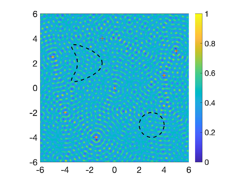
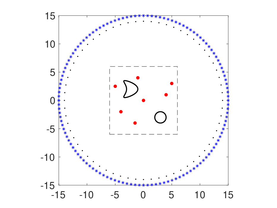
and a unit disk centered at (3,−3)(3,-3). We set k=18,σ=1k=18,\sigma=1 and δ=5%\delta=5\% in this example. The receivers and reference sources are located uniformly on the circle with radii 15 and 14, respectively. For the reconstruction, here a 200×200200\times 200 sampling grid over [−6,6]×[−6,6][-6,6]\times[-6,6] is utilized to image the sources and obstacles. The reconstructions are demonstrated in Figure 4. One could easily observe that the quality of obstacle recovery deteriorates greatly as the number of measurements decreases. At first glance, it seems from Figure 4(c)(d) that the reconstruction of sources is not significantly affected by the reduction of data. However, if we collect the coordinates of local maximizers over the sampling grid and compare them with the exact source points, then it can be immediately seen that the case of insufficient data would produce a mismatched reconstruction of one source point. This comparison is illustrated in Figure 5 where the exact target sources are marked by the small red “+” and the reconstructions are marked by the small black “∘\circ”. These results show that a diminution of the data could lead to incorrect reconstructions, hence the availability of adequate data is essential for the accuracy of recoveries.

Refer to caption
Refer to caption
Refer to caption
Refer to caption
Refer to caption
Refer to caption
Figure 4: Reconstruction of two obstacles and 7 sources. Left column: 256 receivers and 256 reference sources; Right column: 128 receivers and 64 reference sources; Top row: geometry settings of the model; Middle row: imaging of sources; Bottom row: imaging of obstacles.
Refer to caption
Refer to caption
Figure 5: A comparison of the source reconstruction. (a) 256 receivers and 256 reference sources; (b) 128 receivers and 64 reference sources.
Table 1: Reconstruction of source locations in Example 5.3.
Exact locations Reconstruction (more data) Reconstruction (less data)
Point 1 (0,0)(0,0) (0.0302,0.0302)(0.0302,0.0302) (0.0302,0.0302)(0.0302,0.0302)
Point 2 (−1.5,−4)(-1.5,-4) (−1.4774,−4.0101)(-1.4774,-4.0101) (−1.4774,−4.0101)(-1.4774,-4.0101)
Point 3 (5,3)(5,3) (4.9749,2.9849)(4.9749,2.9849) (4.9749,2.9849)(4.9749,2.9849)
Point 4 (−5,2.5)(-5,2.5) (−4.9749,2.5025)(-4.9749,2.5025) (−4.9749,2.5025)(-4.9749,2.5025)
Point 5 (−1,4)(-1,4) (−0.9950,4.0101)(-0.9950,4.0101) (4.0101,−1.4171)(4.0101,-1.4171)
Point 6 (−4,−2)(-4,-2) (−3.9497,−1.9598)(-3.9497,-1.9598) (−3.9497,−1.9598)(-3.9497,-1.9598)
Point 7 (4,1)(4,1) (4.0101,0.9950)(4.0101,0.9950) (4.0101,0.9950)(4.0101,0.9950)

Acknowledgments

D. Zhang and Y. Wu were supported by NSFC grant 12171200 and Y. Guo was supported by NSFC grant 11971133.

References

  • [1] Ammari H, Chow Y T and Zou J 2016 Phased and phaseless domain reconstructions in the inverse scattering problem via scattering coefficients SIAM J. Appl. Math. 76 1000–1030
  • [2] Athanasiadis C, Martin P, Spyropoulos A and Stratis I 2002 Scattering relations for point sources: Acoustic and electromagnetic waves J. Math. Phys 43 5683–5697
  • [3] Bao G, Liu Y and Triki F 2021 Recovering simultaneously a potential and a point source from Cauchy data, Minimax Theory and its Applications 6 227–238
  • [4] Chang Y and Guo Y 2022 Simultaneous recovery of an obstacle and its excitation sources from near-field scattering data Electron. Res. Arch. 30 1296–1321
  • [5] Chen Z and Huang G 2017 Phaseless imaging by reverse time migration: acoustic waves Numer. Math. Theor. Meth. Appl. 10 1–21
  • [6] Colton D and Kress R 2019 Inverse Acoustic and Electromagnetic Scattering Theory 4th ed. (Cham: Springer-Verlag)
  • [7] Dong H, Lai J and Li P 2020 An inverse acoustic-elastic interaction problem with phased or phaseless far-field data Inverse Problems 36 035014
  • [8] Dong H, Zhang D and Guo Y 2019 A reference ball based iterative algorithm for imaging acoustic obstacle from phaseless far-field data Inverse Problems and Imaging 13 177–195.
  • [9] Hu G, Kian Y and Zhao Y 2020 Uniqueness to some inverse source problems for the wave equation in unbounded domains, Acta Mathematicae Applicatae Sinica, English Series 36 134–150
  • [10] Ji X, Liu X and Zhang B 2019 Target reconstruction with a reference point scatterer using phaseless far field patterns, SIAM J. Imaging Sci., 12 372–391
  • [11] Ji X, Liu X and Zhang B 2019 Phaseless inverse source scattering problem: Phase retrieval, uniqueness and direct sampling methods, J. Comput. Phys. X 1 100003
  • [12] Klibanov M V and Romanov V G 2017 Uniqueness of a 3-D coefficient inverse scattering problem without the phase information Inverse Problems 33 095007
  • [13] Li J and Liu H 2015 Recovering a polyhedral obstacle by a few backscattering measurements J. Differential Equat. 259 2101–2120
  • [14] Li J, Liu H, Ma S 2019 Determining a random Schrödinger equation with unknown source and potential SIAM J. Math. Anal. 51 3465–3491
  • [15] Li J, Liu H, Ma S 2021 Determining a random Schrödinger operator: both potential and source are random Comm. Math. Phys. 381 527–556
  • [16] Li J, Liu H and Wang Y 2017 Recovering an electromagnetic obstacle by a few phaseless backscattering measurements Inverse Problems 33 035001
  • [17] Maretzke S and Hohage T, 2017 Stability estimates for linearized near-field phase retrieval in X-ray phase contrast imaging SIAM J. Appl. Math. 77 384–408
  • [18] McLean W 2000 Strongly Elliptic Systems and Boundary Integral Equations (Cambridge: Cambridge University)
  • [19] Novikov R G 2016 Explicit formulas and global uniqueness for phaseless inverse scattering in multidimensions J. Geom. Anal. 26 346–359.
  • [20] Romanov V. G. 2020 Phaseless inverse problems for Schrödinger, Helmholtz, and Maxwell Equations Comput. Math. Math. Phys. 60 1045–1062
  • [21] Sun F, Zhang D and Guo Y 2019 Uniqueness in phaseless inverse scattering problems with known superposition of incident point sources Inverse Problems 35 105007
  • [22] Xu X, Zhang B and Zhang H, 2020 Uniqueness in inverse acoustic and electromagnetic scattering with phaseless near-field data at a fixed frequency, Inverse Probl. Imaging 14 489–510.
  • [23] Zhang D, Guo Y, Sun F and Liu H 2020 Unique determinations in inverse scattering problems with phaseless near-field measurements, Inverse Probl. Imaging, 14 569–582
  • [24] Zhang D, Wang Y, Guo Y and Li J 2020 Uniqueness in inverse cavity scattering problems with phaseless near-field data Inverse Problems 36 025004
  • [25] Zhang D, Guo Y, Li J and Liu H 2018 Retrieval of acoustic sources from multi-frequency phaseless data Inverse Problems 34 094001
  • [26] Zhang D, Guo Y, Wang Y and Chang Y 2022 Co-inversion of a scattering cavity and its internal sources: uniqueness, decoupling and imaging arXiv: 2207.06133
  • [27] Zheng J, Cheng J, Li P and Lu S 2017 Periodic surface identification with phase or phaseless near-field data Inverse Problems 33 115004