跳到论文正文
W Papers独立论文阅读器 arXiv:2212.09322 论文正文 计算阅读时间 · 0%
引用这篇论文根据当前论文元数据生成,正式投稿前建议核对。


License: CC BY-NC-ND 4.0
arXiv:2212.09322v1 [math.NA] 19 Dec 2022

A singularly perturbed convection-diffusion parabolic problem with incompatible boundary/initial dataThanks: This research was partially supported by the Institute of Mathematics and Applications (IUMA), the project PID2019-105979GB-I00 and the Diputación General de Aragón (E24-17R).

J.L. Gracia Thanks: Department of Applied Mathematics, University of Zaragoza, Spain. email: jlgracia@unizar.es    E. O’Riordan Thanks: School of Mathematical Sciences, Dublin City University, Dublin 9, Ireland. email: eugene.oriordan@dcu.ie
August 11, 2026
Abstract

A singularly perturbed parabolic problem of convection-diffusion type with incompatible inflow boundary and initial conditions is examined. In the case of constant coefficients, a set of singular functions are identified which match certain incompatibilities in the data and also satisfy the associated homogenous differential equation. When the convective coefficient only depends on the time variable and the initial/boundary data is discontinuous, then a mixed analytical/numerical approach is taken. In the case of variable coefficients and the zero level of compatibility being satisfied (i.e. continuous boundary/initial data), a numerical method is constructed whose order of convergence is shown to depend on the next level of compatibility being satisfied by the data. Numerical results are presented to support the theoretical error bounds established for both of the approaches examined in the paper.

1 Introduction

Consider the following singularly perturbed parabolic problem: Find uu such that

L​u:=−ε​ux​x+a⁡(x,t)​ux+ut=f⁡(x,t),(x,t)∈G:=(0,1)×(0,T],\displaystyle Lu:=-\varepsilon u_{xx}+a(x,t)u_{x}+u_{t}=f(x,t),\quad(x,t)\in G:=(0,1)\times(0,T], (1a)
u⁡(0,t)=gL​(t),u⁡(1,t)=gR​(t),t>0,u⁡(x,0)=ϕ⁡(x),0≤x≤1;\displaystyle u(0,t)=g_{L}(t),\ u(1,t)=g_{R}(t),\ t>0,\quad u(x,0)=\phi(x),\quad 0\leq x\leq 1; (1b)
a⁡(x,t)≥α>0,(x,t)∈G¯;0<ε≤1.\displaystyle a(x,t)\geq\alpha>0,\ (x,t)\in\bar{G};\quad 0<\varepsilon\leq 1. (1c)
In the case of sufficiently smooth and compatible data, the solution of this problem will contain a boundary layer of width O⁡(ε)O(\varepsilon) near the outflow boundary x=1x=1. Below, we examine the issues that arise when the problem data is not sufficiently compatible at the inflow point (0,0)(0,0). If the boundary and initial conditions are incompatible (ϕ​(0)≠gL​(0)\phi(0)\neq g_{L}(0)), a strong [4] interior layer will appear for small values of the singular perturbation parameter. If ϕ​(0)=gL​(0)\phi(0)=g_{L}(0), but the data are still not sufficiently compatible at (0,0)(0,0) then a weak [4] interior layer appears in the solution. The path of any interior layer is located along the characteristic curve x=d⁡(t)x=d(t), where d⁡(t)d(t) is implicitly defined by
d′​(t)=a⁡(d⁡(t),t),d⁡(0)=0.d^{\prime}(t)=a(d(t),t),\quad d(0)=0.
To avoid the interior layer interacting with the outflow boundary, we assume that at the final time
d⁡(T)<1.d(T)<1. (1d)
See Remark 1 for necessary modifications when (1d) is not satisfied.

Let us recall the constraints on the data, a,f,ϕ,gLa,\,f,\,\phi,\,g_{L} and gRg_{R}, for the solution uu to be sufficiently regular so that classical numerical analysis is applicable; i.e., for u∈C4+γ​(G¯)u\in C^{4+\gamma}(\bar{G})11 1 As in [5], we define the space 𝒞0+γ​(D){\mathcal{C}}^{0+\gamma}(D), where D⊂𝐑2D\subset\mathbf{R}^{2} is an open set, as the set of all functions that are Hölder continuous of degree γ∈(0,1)\gamma\in(0,1) with respect to the metric ∥⋅∥,\|\cdot\|, where for all 𝐩i=(xi,ti),∈𝐑2,i=1,2;∥𝐩1−𝐩2∥2=(x1−x2)2+|t1−t2|{\bf p}_{i}=(x_{i},t_{i}),\in\mathbf{R}^{2},i=1,2;\ \|{\bf p}_{1}-{\bf p}_{2}\|^{2}=(x_{1}-x_{2})^{2}+|t_{1}-t_{2}|. For ff to be in 𝒞0+γ​(D){\mathcal{C}}^{0+\gamma}(D) the following semi-norm needs to be finite ⌈f⌉0+γ,D=sup𝐩1≠𝐩2,𝐩1,𝐩2∈D|f⁡(𝐩1)−f⁡(𝐩2)|‖𝐩1−𝐩2‖γ.\lceil f\rceil_{0+\gamma,D}=\sup_{{\bf p}_{1}\neq{\bf p}_{2},\ {\bf p}_{1},{\bf p}_{2}\in D}\frac{|f({\bf p}_{1})-f({\bf p}_{2})|}{\|{\bf p}_{1}-{\bf p}_{2}\|^{\gamma}}. The space 𝒞n+γ​(D){\mathcal{C}}^{n+\gamma}(D) is defined by 𝒞n+γ(D)={z:∂i+jz∂xi​∂tj∈𝒞0+γ(D), 0≤i+2j≤n},{\mathcal{C}}^{n+\gamma}(D)=\left\{z:\frac{\partial^{i+j}z}{\partial x^{i}\partial t^{j}}\in{\mathcal{C}}^{0+\gamma}(D),\ 0\leq i+2j\leq n\right\}, and ∥⋅∥n+γ,⌈⋅⌉n+γ\|\cdot\|_{n+\gamma},\ \lceil\cdot\rceil_{n+\gamma} are the associated norms and semi-norms. . From [9] we have the following result: If a,f∈C0+γ​(G¯),ϕ∈C2+γ​[0,1],gL,gR∈C1+γ/2​[0,T]a,f\in C^{0+\gamma}(\bar{G}),\,\phi\in C^{2+\gamma}[0,1],\,g_{L},g_{R}\in C^{1+\gamma/2}[0,T] and

A0=0​ with ​A0:=gL​(0)−ϕ⁡(0),\displaystyle A_{0}=0\text{ with }A_{0}:=g_{L}(0)-\phi(0), (2a)
A1=0​ with ​A1:=−ε​ϕ′′​(0)+a⁡(0,0)​ϕ′​(0)+gL′​(0)−f⁡(0,0),\displaystyle A_{1}=0\text{ with }A_{1}:=-\varepsilon\phi^{\prime\prime}(0)+a(0,0)\phi^{\prime}(0)+g_{L}^{\prime}(0)-f(0,0), (2b)
gR​(0)=ϕ⁡(1);−ε​ϕ′′​(1)+a⁡(1,0)​ϕ′​(1)+gR′​(0)=f⁡(1,0),\displaystyle g_{R}(0)=\phi(1);\quad-\varepsilon\phi^{\prime\prime}(1)+a(1,0)\phi^{\prime}(1)+g_{R}^{\prime}(0)=f(1,0), (2c)
then the solution of problem (1) satisfies u∈C2+γ​(G¯)u\in C^{2+\gamma}(\bar{G}). By differentiating with respect to the time variable the differential equation (1a) and applying the above conditions on the function ut​(x,t)u_{t}(x,t), we arrive at the following result: If a,f∈C2+γ​(G¯),ϕ∈C4+γ​[0,1],gl,gR∈C2+γ/2​[0,T]a,f\in C^{2+\gamma}(\bar{G}),\,\phi\in C^{4+\gamma}[0,1],\,g_{l},g_{R}\in C^{2+\gamma/2}[0,T] and in addition to the constraints (2a), (2b) and (2c) we have
A2=0​ with\displaystyle A_{2}=0\text{ with }
A2:=−ε2​ϕ(i​v)​(0)+2​ε​a​(0,0)​ϕ′′′​(0)−a2​(0,0)​ϕ′′​(0)+gL′′​(0−)\displaystyle A_{2}:=-\varepsilon^{2}\phi^{(iv)}(0)+2\varepsilon a(0,0)\phi^{\prime\prime\prime}(0)-a^{2}(0,0)\phi^{\prime\prime}(0)+g_{L}^{\prime\prime}(0^{-})
+ε⁡(ax​x​(0,0)​ϕ′​(0)+2​ax​(0,0)​ϕ′′​(0))+(at−a​ax)​(0,0)​ϕ′​(0)\displaystyle\hskip 8.5359pt+\varepsilon(a_{xx}(0,0)\phi^{\prime}(0)+2a_{x}(0,0)\phi^{\prime\prime}(0))+(a_{t}-aa_{x})(0,0)\phi^{\prime}(0)
−(ft+ε​fx​x−a​fx)​(0,0),\displaystyle\hskip 8.5359pt-(f_{t}+\varepsilon f_{xx}-af_{x})(0,0), (2d)
−ε2​ϕ(i​v)​(1)+2​ε​a​(1,0)​ϕ′′′​(1)−a2​(1,0)​ϕ′′​(1)+gR′′​(0−)\displaystyle-\varepsilon^{2}\phi^{(iv)}(1)+2\varepsilon a(1,0)\phi^{\prime\prime\prime}(1)-a^{2}(1,0)\phi^{\prime\prime}(1)+g_{R}^{\prime\prime}(0^{-})
+ε⁡(ax​x​(1,0)​ϕ′​(1)+2​ax​(1,0)​ϕ′′​(1))+(at−a​ax)​(1,0)​ϕ′​(1)\displaystyle\hskip 8.5359pt+\varepsilon(a_{xx}(1,0)\phi^{\prime}(1)+2a_{x}(1,0)\phi^{\prime\prime}(1))+(a_{t}-aa_{x})(1,0)\phi^{\prime}(1)
=(ft+ε​fx​x−a​fx)​(1,0),\displaystyle\hskip 8.5359pt=(f_{t}+\varepsilon f_{xx}-af_{x})(1,0), (2e)

then the solution of problem (1) satisfies u∈C4+γ​(G¯)u\in C^{4+\gamma}(\bar{G}).

In the case of constant coefficients and when (2a) is not satisfied, the discontinuous analytic solution in the quarter plane x,t>0x,t>0 is given, for example, in [15] and in [1] an asymptotic expansion is given in the domain G¯\bar{G}. In the case of a variable coefficient a⁡(t)a(t) and when (2a) is satisfied, a uniformly valid asymptotic expansion to the continuous solution of the problem posed on the quarter plane is presented in [16].

In this paper, we examine the convection-diffusion problem (1) where the compatibility conditions (2a), (2b) and (2d) at (0,0)(0,0) are not all imposed. To avoid additional regularity issues with the data we will assume that a,f∈C5+γ​(G¯),ϕ∈C7​[0,1],gL∈C5​[0,T],gR∈C3​[0,T]a,f\in C^{5+\gamma}(\bar{G}),\,\phi\in C^{7}[0,1],\,g_{L}\in C^{5}[0,T],g_{R}\in C^{3}[0,T] and that the compatibility conditions (2c) and (2e) at (1,0)(1,0) are all satisfied. We examine the problem where the initial and left boundary condition do not match, i.e., (2a) is not satisfied. In this case, we only examine problem (1) when the convection coefficient a⁡(x,t)a(x,t) depends solely on the time variable. Moreover, we first separate off a singular function that matches the incompatibility at the point (0,0)(0,0) and then use a numerical method to approximate the difference between the solution uu and this singular function.

We also examine the problem where the initial and boundary condition match, so that the zero level compatibility (2a) is satisfied; but the higher compatibility conditions (2b) and (2d) are not satisfied. As the solution is continuous, a numerical method can be applied directly to the problem. If (2a) is satisfied but the first level of compatibility (2b) is not satisfied, then the order of convergence of the standard numerical method constructed in §4 is shown to be 0.50.5. If the first level of compatibility (2a) and (2b) is satisfied, then that numerical method is essentially first order.

In [6] and [7], the parabolic problem (1) with compatible boundary/initial data is examined, but with a discontinuity in the initial condition ϕ⁡(x)\phi(x) at some internal point x=d, 0<d<1x=d,\,0<d<1. In this case, the interior layer function

0.5​erfc⁡(d⁡(t)−x2​ε​t), 0<d⁡(0)<1,erfc⁡(z):=2π​∫r=z∞e−r2​𝑑r,0.5\erfc\left(\frac{d(t)-x}{2\sqrt{\varepsilon t}}\right),\ 0<d(0)<1,\quad\erfc(z):=\frac{2}{\sqrt{\pi}}\int_{r=z}^{\infty}e^{-r^{2}}dr,

captures the nature of the singularity. In §2 a set of related functions Sn​(x,t),n≥0S_{n}(x,t),n\geq 0 are constructed to model the nature of any singularity in the solution related to a lack of compatibility between the initial and boundary condition at the point (0,0)(0,0). Parameter-explicit pointwise bounds on the partial derivatives of these functions are also established in §2. In §3, the solution uu of (1) is expanded in terms of these special functions Sn​(x,t)S_{n}(x,t) as follows:

u⁡(x,t)=∑i=01Ai​Si​(x,t)+∑i=23Bi​Si​(x,t)+v⁡(x,t)+w⁡(x,t),u(x,t)=\sum_{i=0}^{1}A_{i}S_{i}(x,t)+\sum_{i=2}^{3}B_{i}S_{i}(x,t)+v(x,t)+w(x,t),

where the amplitudes Ai,i=0,1;Bi,i=2,3A_{i},\,i=0,1;B_{i},\ i=2,3 are suitably chosen so that v,w∈C4+γ​(G¯)v,w\in C^{4+\gamma}(\bar{G}), where vv is the regular component and ww is the boundary layer component of the solution uu. With the aid of this expansion, a numerical method is constructed in §4 to generate a numerical approximation to u−A0​S0u-A_{0}S_{0} (including also the case A0=0A_{0}=0). The order of convergence of this method depends on whether A1A_{1} is zero or not. In §5, numerical results are presented for sample test problems to illustrate the performance of the method and to validate the orders of convergence established in the two main Theorems 3 and 4 in §4. Technical details associated with establishing bounds on the derivatives of the functions Sn​(x,t)S_{n}(x,t) are given in the appendix.

Notation: Throughout the paper, CC denotes a generic constant that is independent of the singular perturbation parameter ε\varepsilon and all the discretization parameters. The L∞L_{\infty} norm on the domain DD will be denoted by ∥⋅∥D\|\cdot\|_{D}. We also define the following interior layer function

Eγ​(x,t):=e−γ​(x−d⁡(t))24​ε​t,0<γ≤1.E_{\gamma}(x,t):=e^{-\frac{\gamma(x-d(t))^{2}}{4\varepsilon t}},\quad 0<\gamma\leq 1.

If γ=1\gamma=1, we simply write E1​(x,t)=E⁡(x,t)E_{1}(x,t)=E(x,t).

2 A set of singular functions with incompatiblities

We now define a set of singular functions Sn​(x,t)S_{n}(x,t), which will form a basis for the regularity expansion of the solution u⁡(x,t)u(x,t) of problem (1), which is constructed in Theorem 1 (for A0≠0A_{0}\neq 0 and a=a⁡(t)a=a(t)) and Theorem 2 (for A0=0A_{0}=0 and a=a⁡(x,t)a=a(x,t)). For all n≥0n\geq 0:

Sn​(x,t):=ψn+​(x,t)+(−1)n​ψn−​(x,t)an​(0,0),S_{n}(x,t):=\frac{\psi_{n}^{+}(x,t)+(-1)^{n}\psi^{-}_{n}(x,t)}{a^{n}(0,0)}, (3)

where the functions ψn±​(x,t),n≥−1\psi^{\pm}_{n}(x,t),n\geq-1 are defined by

ψn−​(x,t)\displaystyle\psi^{-}_{n}(x,t) :=(−1)n​2n−1​n!​(ε​t)n/2​erfcn⁡(χ−​(x,t)),\displaystyle:=(-1)^{n}2^{n-1}n!(\varepsilon t)^{n/2}\erfc_{n}(\chi^{-}(x,t)), (4a)
ψn+​(x,t)\displaystyle\psi^{+}_{n}(x,t) :=(−1)n​2n−1​n!​(ε​t)n/2​ex​d​(t)ε​t​erfcn⁡(χ+​(x,t)),\displaystyle:=(-1)^{n}2^{n-1}n!(\varepsilon t)^{n/2}e^{\frac{xd(t)}{\varepsilon t}}\erfc_{n}(\chi^{+}(x,t)), (4b)
χ±​(x,t)\displaystyle\chi^{\pm}(x,t) :=x±d⁡(t)2​ε​t,ψ−1±​(x,t):=−E⁡(x,t)2​ε​π​t,\displaystyle:=\frac{x\pm d(t)}{2\sqrt{\varepsilon t}},\quad\psi_{-1}^{\pm}(x,t):=-\frac{E(x,t)}{2\sqrt{\varepsilon\pi t}}, (4c)

and the iterated complementary error functions are

erfc−1⁡(x):=2π​e−x2,erfcn⁡(x):=∫s=x∞erfcn−1⁡(s)​𝑑s,n≥0.\erfc_{-1}(x):=\frac{2}{\sqrt{\pi}}e^{-x^{2}},\quad\erfc_{n}(x):=\int_{s=x}^{\infty}\erfc_{n-1}(s)\,ds,\quad n\geq 0.

Observe that the first function S0S_{0} is discontinuous and

S1∈C0+γ​(G¯),S2​n,S2​n+1∈C2​n+γ​(G¯),n≥1.S_{1}\in C^{0+\gamma}(\bar{G}),\qquad S_{2n},S_{2n+1}\in C^{2n+\gamma}(\bar{G}),\quad n\geq 1.

In the next lemma, we establish bounds on the derivatives of the first three functions Sn,n=0,1,2.S_{n},\,n=0,1,2. These bounds indicate both the strength of the singularity at t=0t=0 and how certain derivatives can depend on inverse powers of ε\varepsilon.

Lemma 1.

The function S0​(x,t)S_{0}(x,t) satisfies the bounds

|S0|≤C,|∂iS0∂ti|≤C[1t(1+tε)]iEγ(x,t),i=1,2,\displaystyle|S_{0}|\leq C,\quad\left|\frac{\partial^{i}S_{0}}{\partial t^{i}}\right|\leq C\left[\frac{1}{t}\left(1+\sqrt{\frac{t}{\varepsilon}}\right)\right]^{i}E_{\gamma}(x,t),\quad i=1,2, (5a)
|∂iS0∂xi|≤Cεi(εt+(εt)i/2)Eγ(x,t),i=1,2,3;\displaystyle\left|\frac{\partial^{i}S_{0}}{\partial x^{i}}\right|\leq\frac{C}{\varepsilon^{i}}\left(\frac{\varepsilon}{t}+\left(\frac{\varepsilon}{t}\right)^{i/2}\right)E_{\gamma}(x,t),\quad i=1,2,3; (5b)

the function S1​(x,t)S_{1}(x,t) satisfies

|S1|≤C,|∂S1∂t|≤C,|∂2S1∂t2|≤C​1t​(1+tε)​Eγ​(x,t)+C,\displaystyle|S_{1}|\leq C,\quad\left|\frac{\partial S_{1}}{\partial t}\right|\leq C,\ \left|\frac{\partial^{2}S_{1}}{\partial t^{2}}\right|\leq C\frac{1}{t}\left(1+\sqrt{\frac{t}{\varepsilon}}\right)E_{\gamma}(x,t)+C, (6a)
|∂S1∂x|≤C,|∂2S1∂x2|≤Cε​Eγ​(x,t)+C,|∂3S1∂x3|≤Cε​ε​t​Eγ​(x,t)+C;\displaystyle\left|\frac{\partial S_{1}}{\partial x}\right|\leq C,\ \left|\frac{\partial^{2}S_{1}}{\partial x^{2}}\right|\leq\frac{C}{\varepsilon}E_{\gamma}(x,t)+C,\ \left|\frac{\partial^{3}S_{1}}{\partial x^{3}}\right|\leq\frac{C}{\varepsilon\sqrt{\varepsilon t}}E_{\gamma}(x,t)+C; (6b)

and the function S2​(x,t)S_{2}(x,t) satisfies

|S2|≤C,|∂S2∂x|≤C,\displaystyle|S_{2}|\leq C,\quad\left|\frac{\partial S_{2}}{\partial x}\right|\leq C, (7a)
|∂S2∂t|≤C,|∂2S2∂t2|≤C⁡(1+εt)​(1+tε)​Eγ​(x,t)+C,\displaystyle\left|\frac{\partial S_{2}}{\partial t}\right|\leq C,\ \left|\frac{\partial^{2}S_{2}}{\partial t^{2}}\right|\leq C\left(1+\frac{\varepsilon}{t}\right)\left(1+\sqrt{\frac{t}{\varepsilon}}\right)E_{\gamma}(x,t)+C, (7b)
|∂2S2∂x2|≤C⁡(1+tε)​Eγ​(x,t),\displaystyle\left|\frac{\partial^{2}S_{2}}{\partial x^{2}}\right|\leq C\left(1+\sqrt{\frac{t}{\varepsilon}}\right)E_{\gamma}(x,t), (7c)
|∂3S2∂x3|≤Cε​(1+tε+εt)​Eγ​(x,t).\displaystyle\left|\frac{\partial^{3}S_{2}}{\partial x^{3}}\right|\leq\frac{C}{\varepsilon}\left(1+\sqrt{\frac{t}{\varepsilon}}+\sqrt{\frac{\varepsilon}{t}}\right)E_{\gamma}(x,t). (7d)
Proof.

In the appendix, bounds on the partial derivatives of the functions ψn±​(x,t)\psi^{\pm}_{n}(x,t) are established. These are used to prove the bounds on SnS_{n}. The bounds on S0S_{0} follow directly from (26) and (30). Using (23a) and the recurrence relation (24) we deduce the following

∂S1∂t\displaystyle\frac{\partial S_{1}}{\partial t} =a⁡(d⁡(t),t)a⁡(0,0)​S0+x​p⁡(t)​ψ1+ε​t2,p⁡(t):=t​a​(d⁡(t),t)−d⁡(t);\displaystyle=\frac{a(d(t),t)}{a(0,0)}S_{0}+x\frac{p(t)\psi^{+}_{1}}{\varepsilon t^{2}},\quad p(t):=ta(d(t),t)-d(t);
a2​(0,0)​∂S2∂t\displaystyle a^{2}(0,0)\frac{\partial S_{2}}{\partial t} =2​(ε​S0−a⁡(0,0)​a​(d⁡(t),t)​S1+d⁡(t)t​ψ1+)−p⁡(t)ε​t2​(d⁡(t)​ψ2+−ψ3+).\displaystyle=2(\varepsilon S_{0}-a(0,0)a(d(t),t)S_{1}+\frac{d(t)}{t}\psi^{+}_{1})-\frac{p(t)}{\varepsilon t^{2}}(d(t)\psi^{+}_{2}-\psi^{+}_{3}).

The bounds on the time derivatives of S1S_{1} and S2S_{2} follow. To deduce the bounds on the space derivatives of these components, we first note that from (24), we have

a⁡(0,0)​∂S1∂x\displaystyle a(0,0)\frac{\partial S_{1}}{\partial x} =ψ0+−ψ0−+d⁡(t)ε​t​ψ1+,\displaystyle=\psi^{+}_{0}-\psi^{-}_{0}+\frac{d(t)}{\varepsilon t}\psi_{1}^{+},
a⁡(0,0)​∂2S1∂x2\displaystyle a(0,0)\frac{\partial^{2}S_{1}}{\partial x^{2}} =d⁡(t)t​ε​(2​ψ0++d⁡(t)t​ε​ψ1+),\displaystyle=\frac{d(t)}{t\varepsilon}\left(2\psi^{+}_{0}+\frac{d(t)}{t\varepsilon}\psi^{+}_{1}\right),
a⁡(0,0)​∂3S1∂x3\displaystyle a(0,0)\frac{\partial^{3}S_{1}}{\partial x^{3}} =d⁡(t)t​ε​(2​∂ψ0+∂x+d⁡(t)t​ε​(ψ0++d⁡(t)t​ε​ψ1+)),\displaystyle=\frac{d(t)}{t\varepsilon}\left(2\frac{\partial\psi^{+}_{0}}{\partial x}+\frac{d(t)}{t\varepsilon}\left(\psi^{+}_{0}+\frac{d(t)}{t\varepsilon}\psi^{+}_{1}\right)\right),

and from (31) the bounds on the space derivatives of S1S_{1} follow. Next, we deduce bounds on the space derivatives of S2S_{2}. From the definitions in (4), the following bounds are obtained

|∂iψj−∂xi|≤C(ε​t)j−iEγ(x,t)+C,j=1,2;i=1,2,3,\left|\frac{\partial^{i}\psi^{-}_{j}}{\partial x^{i}}\right|\leq C(\sqrt{\varepsilon t})^{j-i}E_{\gamma}(x,t)+C,\quad j=1,2;\quad i=1,2,3,

and using the recurrence relation (24) we get the bounds

|∂ψ1+∂x|≤C​Eγ​(x,t),|∂2ψ1+∂x2|≤Cε​(1+εt)​Eγ​(x,t),\displaystyle\left|\frac{\partial\psi^{+}_{1}}{\partial x}\right|\leq CE_{\gamma}(x,t),\ \left|\frac{\partial^{2}\psi^{+}_{1}}{\partial x^{2}}\right|\leq\frac{C}{\varepsilon}\left(1+\sqrt{\frac{\varepsilon}{t}}\right)E_{\gamma}(x,t), (8a)
|∂3ψ1+∂x3|≤Cε​t​(1+tε)​Eγ​(x,t),\displaystyle\left|\frac{\partial^{3}\psi^{+}_{1}}{\partial x^{3}}\right|\leq\frac{C}{\varepsilon t}\left(1+\sqrt{\frac{t}{\varepsilon}}\right)E_{\gamma}(x,t), (8b)
|∂ψ2+∂x|≤C​ε​t​Eγ​(x,t),|∂2ψ2+∂x2|≤C⁡(1+tε)​Eγ​(x,t),\displaystyle\left|\frac{\partial\psi^{+}_{2}}{\partial x}\right|\leq C\sqrt{\varepsilon t}E_{\gamma}(x,t),\quad\left|\frac{\partial^{2}\psi^{+}_{2}}{\partial x^{2}}\right|\leq C\left(1+\sqrt{\frac{t}{\varepsilon}}\right)E_{\gamma}(x,t), (8c)
|∂3ψ2+∂x3|≤Cε​(1+tε+εt)​Eγ​(x,t).\displaystyle\left|\frac{\partial^{3}\psi^{+}_{2}}{\partial x^{3}}\right|\leq\frac{C}{\varepsilon}\left(1+\sqrt{\frac{t}{\varepsilon}}+\sqrt{\frac{\varepsilon}{t}}\right)E_{\gamma}(x,t). (8d)

The bounds on the space derivatives of S2S_{2} follow immediately from the bounds above on the space derivatives of the singular functions ψi−\psi^{-}_{i} and ψi+\psi_{i}^{+}.

∎

Observe that the strength of the singularity at (0,0)(0,0) in each of the functions SnS_{n} weakens as nn increases. Using the identities in (24), we can deduce bounds on the remaining functions Sn,n≥3S_{n},\,n\geq 3:

|∂Sn∂x|≤C,n≥2,|∂2Sn∂x2|≤C,n≥4,|∂3Sn∂x3|≤C,n≥6,\displaystyle\left|\frac{\partial S_{n}}{\partial x}\right|\leq C,\ n\geq 2,\quad\left|\frac{\partial^{2}S_{n}}{\partial x^{2}}\right|\leq C,\ n\geq 4,\quad\left|\frac{\partial^{3}S_{n}}{\partial x^{3}}\right|\leq C,\ n\geq 6, (9a)
|∂2S3∂x2|≤C⁡(1+t⁡(1+tε)​Eγ​(x,t)),\displaystyle\left|\frac{\partial^{2}S_{3}}{\partial x^{2}}\right|\leq C\left(1+t\left(1+\sqrt{\frac{t}{\varepsilon}}\right)E_{\gamma}(x,t)\right), (9b)
|∂3S3+n∂x3|≤C(1+tn(1+tε)3−nEγ(x,t)),n=0,1,2,\displaystyle\left|\frac{\partial^{3}S_{3+n}}{\partial x^{3}}\right|\leq C\left(1+t^{n}\left(1+\sqrt{\frac{t}{\varepsilon}}\right)^{3-n}E_{\gamma}(x,t)\right),\quad n=0,1,2, (9c)
|∂Sn∂t|≤C,n≥2,|∂2S3∂t2|≤C⁡(1+εt​Eγ​(x,t)),|∂2Sn∂t2|≤C,n≥4.\displaystyle\left|\frac{\partial S_{n}}{\partial t}\right|\leq C,\ n\geq 2,\ \left|\frac{\partial^{2}S_{3}}{\partial t^{2}}\right|\leq C\left(1+\sqrt{\frac{\varepsilon}{t}}E_{\gamma}(x,t)\right),\left|\frac{\partial^{2}S_{n}}{\partial t^{2}}\right|\leq C,\ n\geq 4. (9d)

3 The continuous problem

In the following result the asymptotic behaviour of the solution uu to problem (1) is given when the convective coefficient aa depends only on the time variable and uu is discontinuous at (0,0)(0,0).

Theorem 1.

Assume that a⁡(x,t)=a⁡(t),∀(x,t)∈G¯a(x,t)=a(t),\,\forall(x,t)\in\bar{G} and at​(0)=0a_{t}(0)=0. The solution uu of (1) can be expanded as follows

u⁡(x,t)=∑i=01Ai​Si​(x,t)+∑i=23Bi​Si​(x,t)+v⁡(x,t)+w⁡(x,t),u(x,t)=\sum_{i=0}^{1}A_{i}S_{i}(x,t)+\sum_{i=2}^{3}B_{i}S_{i}(x,t)+v(x,t)+w(x,t), (10a)
where the constants AiA_{i} are defined in (2a) and (2b). The constants B2,B3B_{2},B_{3} are defined such that for 0≤i+2​j≤40\leq i+2j\leq 4
|∂iv∂xi|\displaystyle\left|\frac{\partial^{i}v}{\partial x^{i}}\right| ≤C⁡(1+ε2−i),|∂jv∂tj|≤C;\displaystyle\leq C(1+\varepsilon^{2-i}),\quad\left|\frac{\partial^{j}v}{\partial t^{j}}\right|\leq C; (10b)
|∂i+jw∂xi​∂tj|\displaystyle\left|\frac{\partial^{i+j}w}{\partial x^{i}\partial t^{j}}\right| ≤Cε−i(1+ε1−j)e−α(1−x)/ε.\displaystyle\leq C\varepsilon^{-i}(1+\varepsilon^{1-j})e^{-\alpha(1-x)/\varepsilon}. (10c)
Proof.

With the assumptions a=a⁡(t),at​(0)=0a=a(t),\,a_{t}(0)=0 and noting (23d), we have

LSi=p(t)ψi+1+ε​t2,p(t)=t3P(t),|P(t)|≤CandLS0∈C2+γ(G¯).LS_{i}=p(t)\frac{\psi^{+}_{i+1}}{\varepsilon t^{2}},\ p(t)=t^{3}P(t),\ |P(t)|\leq C\quad\hbox{and}\quad LS_{0}\in C^{2+\gamma}(\bar{G}). (11)

We identify the remainder RR by

R:=u⁡(x,t)−∑i=01Ai​Si​(x,t),R⁡(0,t)=gL​(t)−CL​(t),R⁡(x,0)=ϕ⁡(x),R:=u(x,t)-\sum_{i=0}^{1}A_{i}S_{i}(x,t),\quad R(0,t)=g_{L}(t)-C_{L}(t),\ R(x,0)=\phi(x),

where

CL​(t):=∑i=01Ai​Si​(0,t)=∑i=01Ai​(d⁡(t)a⁡(0))i.C_{L}(t):=\sum_{i=0}^{1}A_{i}S_{i}(0,t)=\sum_{i=0}^{1}A_{i}\left(\frac{d(t)}{a(0)}\right)^{i}.

Then CL​(0)=A0,CL′​(0)=A1C_{L}(0)=A_{0},\ C_{L}^{\prime}(0)=A_{1} and the remainder function RR satisfies

L​R=f−p⁡(t)ε​t2​(A0​ψ1++A1a⁡(0)​ψ2+)∈C2+γ​(G¯).LR=f-\frac{p(t)}{\varepsilon t^{2}}\left(A_{0}\psi^{+}_{1}+\frac{A_{1}}{a(0)}\psi^{+}_{2}\right)\in C^{2+\gamma}(\bar{G}). (12)

Hence, R∈C2+γ​(G¯)R\in C^{2+\gamma}(\bar{G}) as the amplitudes Ai,i=0,1A_{i},i=0,1 have been chosen so that the compatibility conditions (2a) and (2b) are satisfied by the problem data defining RR.

The remainder RR is further decomposed as follows

R⁡(x,t)=∑n=25Bn​Sn​(x,t)+z⁡(x,t)+vS​(x,t)+w⁡(x,t),R(x,t)=\sum_{n=2}^{5}B_{n}S_{n}(x,t)+z(x,t)+v_{S}(x,t)+w(x,t),

with z,vS,w∈C4+γ​(G¯)z,v_{S},w\in C^{4+\gamma}(\bar{G}). The regular component vv of the remainder RR will be determined by v=∑n=45Bn​Sn​(x,t)+z+vSv=\sum_{n=4}^{5}B_{n}S_{n}(x,t)+z+v_{S} and the functions zz and vSv_{S} are required in our decomposition due to the weak singular right-hand side of the differential equation (12). The boundary layer function ww of RR will satisfy the problem L​w=0,w⁡(0,t)=w⁡(x,0)=0,w⁡(1,t)≠0Lw=0,w(0,t)=w(x,0)=0,w(1,t)\neq 0. All these functions and the constants BnB_{n} are specified below.

Consider the following function

z⁡(x,t):=ϕ⁡(x)+z0​(x,t)+ε​z1​(x,t)+ε2​Rz​(x,t);z(x,t):=\phi(x)+z_{0}(x,t)+\varepsilon z_{1}(x,t)+\varepsilon^{2}R_{z}(x,t);

where

L0​z0=f+ε​ϕ′′​(x)−a⁡(t)​ϕ′​(x), 0<x≤1,t>0,\displaystyle L_{0}z_{0}=f+\varepsilon\phi^{\prime\prime}(x)-a(t)\phi^{\prime}(x),\ 0<x\leq 1,\ t>0,
z0​(0,t)=gL​(t)−CL​(t)−ϕ⁡(0)−∑n=25Bn​Sn​(0,t),t>0,z0​(x,0)=0, 0≤x≤1,\displaystyle z_{0}(0,t)=g_{L}(t)-C_{L}(t)-\phi(0)-\sum_{n=2}^{5}B_{n}S_{n}(0,t),\ t>0,\ z_{0}(x,0)=0,\ 0\leq x\leq 1,
L0​z1=∂2z0∂x2, 0<x≤1,t>0,z1​(0,t)=0,t>0,z1​(x,0)=0, 0≤x≤1,\displaystyle L_{0}z_{1}=\frac{\partial^{2}z_{0}}{\partial x^{2}},\ 0<x\leq 1,\ t>0,\ z_{1}(0,t)=0,\ t>0,\ z_{1}(x,0)=0,\ 0\leq x\leq 1,
L​Rz=∂2z1∂x2,(x,t)∈G,Rz​(0,t)=Rz​(1,t)=0,t>0,Rz​(x,0)=0, 0≤x≤1,\displaystyle LR_{z}=\frac{\partial^{2}z_{1}}{\partial x^{2}},\ (x,t)\in G,\ R_{z}(0,t)=R_{z}(1,t)=0,\ t>0,\ R_{z}(x,0)=0,\ 0\leq x\leq 1,

with the reduced differential operator

L0:=∂∂t+a⁡(t)​∂∂x.L_{0}:=\frac{\partial}{\partial t}+a(t)\frac{\partial}{\partial x}.

From this construction, z⁡(1,t)=z0​(1,t)+ε​z1​(1,t)z(1,t)=z_{0}(1,t)+\varepsilon z_{1}(1,t) and

L​z=f,z⁡(0,t)=R⁡(0,t)−∑n=25Bn​Sn​(0,t),z⁡(x,0)=R⁡(x,0).\displaystyle Lz=f,\quad z(0,t)=R(0,t)-\sum_{n=2}^{5}B_{n}S_{n}(0,t),\ z(x,0)=R(x,0).

Note that the function z0z_{0} satisfies z0​(0+,0)=z0​(0,0+)z_{0}(0^{+},0)=z_{0}(0,0^{+}) and the first level compatibility condition

f⁡(0,0)+ε​ϕ′′​(0)−a⁡(0)​ϕ′​(0)=gL′​(0)−CL′​(0),f(0,0)+\varepsilon\phi^{\prime\prime}(0)-a(0)\phi^{\prime}(0)=g_{L}^{\prime}(0)-C_{L}^{\prime}(0),

is satisfied automatically. Hence, from [2] and [11], the function z0z_{0} belongs to the space22 2 The space 𝒞n,γ​(D){\mathcal{C}}^{n,\gamma}(D) is defined by 𝒞n,γ(D)={z:∂i+jz∂xi​∂tj∈𝒞0+γ(D), 0≤i+j≤n},{\mathcal{C}}^{n,\gamma}(D)=\left\{z:\frac{\partial^{i+j}z}{\partial x^{i}\partial t^{j}}\in{\mathcal{C}}^{0+\gamma}(D),\ 0\leq i+j\leq n\right\}, C1,γ​(G¯),C^{1,\gamma}(\bar{G}), due to the particular definition of z0z_{0}.

Now the parameters Bn,n=2,3,4,5B_{n},n=2,3,4,5 are chosen so that the necessary compatibility conditions on the reduced solution z0z_{0} are imposed in order that z0∈C5,γ​(G¯)z_{0}\in C^{5,\gamma}(\bar{G}). Then, z1∈C4,γ​(G¯)z_{1}\in C^{4,\gamma}(\bar{G}) and Rz∈C4+γ​(G¯)R_{z}\in C^{4+\gamma}(\bar{G}). Hence, z∈C4+γ​(G¯)z\in C^{4+\gamma}(\bar{G}) and

|∂i+jz∂xi​∂tj|≤C⁡(1+ε2−i),0≤i+2​j≤4.\left|\frac{\partial^{i+j}z}{\partial x^{i}\partial t^{j}}\right|\leq C\left(1+\varepsilon^{2-i}\right),\quad 0\leq i+2j\leq 4.

We next define the component vSv_{S} as the solution of the initial-boundary value problem

L​vS\displaystyle Lv_{S} =LR−Lz−∑n=25BnLSn=−∑n=01AnLSn−∑n=25BnLSn,(x,t)∈G,\displaystyle=LR-Lz-\sum_{n=2}^{5}B_{n}LS_{n}=-\sum_{n=0}^{1}A_{n}LS_{n}-\sum_{n=2}^{5}B_{n}LS_{n},\quad(x,t)\in G,
vS​(0,t)\displaystyle v_{S}(0,t) =vS​(1,t)=0,t>0,vS​(x,0)=0, 0≤x≤1.\displaystyle=v_{S}(1,t)=0,\,t>0,\quad v_{S}(x,0)=0,\,0\leq x\leq 1.

Observe that vS∈C4+γ​(G¯)v_{S}\in C^{4+\gamma}(\bar{G}) as

(L​vS)​(0,0)=(L​vS)x​(0,0)=(L​vS)x​x​(0,0)=(L​vS)t​(0,0)=0,(Lv_{S})(0,0)=(Lv_{S})_{x}(0,0)=(Lv_{S})_{xx}(0,0)=(Lv_{S})_{t}(0,0)=0,

and L​vS∈C2+γ​(G¯)Lv_{S}\in C^{2+\gamma}(\bar{G}). To deduce bounds on the derivatives of the component vSv_{S} consider the stretched variables

τ=tε,ζ=xε\tau=\frac{t}{\varepsilon},\ \zeta=\frac{x}{\varepsilon} (13)

and we denote g~​(ζ,τ):=g​(x,t)\tilde{g}(\zeta,\tau):=g(x,t) for any function gg. Then, we have

x+d⁡(t)2​ε​t=ζ+d~1​(τ)2​τ, with ​d~1​(τ):=1ε​∫s=0ε​τa⁡(s)​𝑑s=∫s=0τa~​(s)​𝑑s.\frac{x+d(t)}{2\sqrt{\varepsilon t}}=\frac{\zeta+\tilde{d}_{1}(\tau)}{2\sqrt{\tau}},\ \text{ with }\ \tilde{d}_{1}(\tau):=\frac{1}{\varepsilon}\int_{s=0}^{\varepsilon\tau}a(s)\ ds=\int_{s=0}^{\tau}\tilde{a}(s)\ ds.

Using (11), we have that

−∂2v~S∂ζ2+a~​(τ)​∂v~S∂ζ+∂v~S∂τ=−ε2​Φ~+​(ζ,τ),-\frac{\partial^{2}\tilde{v}_{S}}{\partial\zeta^{2}}+\tilde{a}(\tau)\frac{\partial\tilde{v}_{S}}{\partial\zeta}+\frac{\partial\tilde{v}_{S}}{\partial\tau}=-\varepsilon^{2}\tilde{\Phi}^{+}(\zeta,\tau),

where

Φ~+​(ζ,τ):=τ​P~​(τ)​(∑n=01An​ψ~n+1+ε+∑n=25Bn​ψ~n+1+ε).\tilde{\Phi}^{+}(\zeta,\tau):=\tau\tilde{P}(\tau)\left(\sum_{n=0}^{1}\frac{A_{n}\tilde{\psi}^{+}_{n+1}}{\varepsilon}+\sum_{n=2}^{5}\frac{B_{n}\tilde{\psi}^{+}_{n+1}}{\varepsilon}\right).

Then, from the definition (4) of the basic functions ψn−\psi^{-}_{n} and ψn+\psi^{+}_{n}, we have

|∂i+jΦ~+∂ζi​∂τj|≤C,0≤i+2​j≤2.\left|\frac{\partial^{i+j}\tilde{\Phi}^{+}}{\partial\zeta^{i}\partial\tau^{j}}\right|\leq C,\quad 0\leq i+2j\leq 2.

From [5] and [9], we have the following estimates for the partial derivatives of v~S\tilde{v}_{S}

|∂i+jv~S∂ζi​∂τj|≤C​ε2,0≤i+2​j≤4.\left|\frac{\partial^{i+j}\tilde{v}_{S}}{\partial\zeta^{i}\partial\tau^{j}}\right|\leq C\varepsilon^{2},\quad 0\leq i+2j\leq 4.

Returning to the original variables, we get that

|∂i+jvS∂xi​∂tj|≤C⁡(1+ε2−(i+j)),0≤i+2​j≤4.\left|\frac{\partial^{i+j}v_{S}}{\partial x^{i}\partial t^{j}}\right|\leq C\left(1+\varepsilon^{2-(i+j)}\right),\quad 0\leq i+2j\leq 4.

We can now define the regular component v∈C4+γ​(G¯)v\in C^{4+\gamma}(\bar{G}) to be

v⁡(x,t):=z⁡(x,t)+vS​(x,t)+∑n=45Bn​Sn​(x,t).v(x,t):=z(x,t)+v_{S}(x,t)+\sum_{n=4}^{5}B_{n}S_{n}(x,t).

Finally, consider the boundary layer component ww; it is the solution of

L​w\displaystyle Lw =0,(x,t)∈G,\displaystyle=0,\quad(x,t)\in G,
w⁡(0,t)\displaystyle w(0,t) =0,w⁡(1,t)=(R−v−∑n=23Bn​Sn)​(1,t),t>0,\displaystyle=0,\ w(1,t)=\left(R-v-\sum_{n=2}^{3}B_{n}S_{n}\right)(1,t),\ t>0,
w⁡(x,0)\displaystyle w(x,0) =0, 0≤x≤1.\displaystyle=0,\ 0\leq x\leq 1.

The bounds on ww are established as in [8, Theorem 1]. We note that we require the assumption (1d) to establish the bounds on the derivatives of the boundary layer function ww. This assumption guarantees that d⁡(T)<1d(T)<1 and then the interior and boundary layers do not interact with each other.

∎

In the next theorem, we consider the case where (2a) is satisfied and the solution is continuous. In this case we can relax the constraints on the coefficient a⁡(x,t)a(x,t) and allow this coefficient to vary in both space and time.

Theorem 2.

Assume that ax​(0,0)=0a_{x}(0,0)=0 and gL​(0)=ϕ​(0)g_{L}(0)=\phi(0). The solution uu of (1) can be expanded as follows:

u⁡(x,t)=A1​S1​(x,t)+∑i=23Bi​Si​(x,t)+v⁡(x,t)+w⁡(x,t),u(x,t)=A_{1}S_{1}(x,t)+\sum_{i=2}^{3}B_{i}S_{i}(x,t)+v(x,t)+w(x,t), (14a)
where A1A_{1} is defined in (2b) and for 0≤i+2​j≤40\leq i+2j\leq 4
|∂iv∂xi|\displaystyle\left|\frac{\partial^{i}v}{\partial x^{i}}\right| ≤C⁡(1+ε2−i),|∂jv∂tj|≤C,\displaystyle\leq C(1+\varepsilon^{2-i}),\quad\left|\frac{\partial^{j}v}{\partial t^{j}}\right|\leq C, (14b)
|∂i+jw∂xi​∂tj|\displaystyle\left|\frac{\partial^{i+j}w}{\partial x^{i}\partial t^{j}}\right| ≤Cε−i(1+ε1−j)e−α(1−x)/ε.\displaystyle\leq C\varepsilon^{-i}(1+\varepsilon^{1-j})e^{-\alpha(1-x)/\varepsilon}. (14c)
Proof.

Follow the argument in Theorem 2, but now we define the remainder to be R:=u⁡(x,t)−A1​S1​(x,t)R:=u(x,t)-A_{1}S_{1}(x,t) which satisfies

L​R=f−p⁡(t)ε​t2​A1a⁡(0,0)​ψ2+−(a⁡(x,t)−a⁡(d⁡(t),t))​A1​∂S1∂x.LR=f-\frac{p(t)}{\varepsilon t^{2}}\frac{A_{1}}{a(0,0)}\psi^{+}_{2}-(a(x,t)-a(d(t),t))A_{1}\frac{\partial S_{1}}{\partial x}. (15)

We examine the regularity of the function RR. Compare (15) with (12). As in Theorem 1, the term f−p⁡(t)ε​t2​A1a⁡(0,0)​ψ2+f-\frac{p(t)}{\varepsilon t^{2}}\frac{A_{1}}{a(0,0)}\psi^{+}_{2} in the right-hand side of (15) belongs to C2+γ​(G¯)C^{2+\gamma}(\bar{G}) since ψ2+​(x,t)∈C2+γ​(G¯)\psi^{+}_{2}(x,t)\in C^{2+\gamma}(\bar{G}). We now consider the other term (a⁡(x,t)−a⁡(d⁡(t),t))​A1​∂S1∂x(a(x,t)-a(d(t),t))A_{1}\frac{\partial S_{1}}{\partial x} of (15). Observe that, if ax​(0,0)=0a_{x}(0,0)=0 then

a⁡(x,t)−a⁡(d⁡(t),t)\displaystyle a(x,t)-a(d(t),t) =∫s=d⁡(t)xax​(s,t)​𝑑s\displaystyle=\int_{s=d(t)}^{x}a_{x}(s,t)\,ds
=∫s=d⁡(t)x∫r=0tax​t​(s,r)​𝑑r​𝑑s+∫s=d⁡(t)x∫r=0sax​x​(r,0)​𝑑r​𝑑s.\displaystyle=\int_{s=d(t)}^{x}\int_{r=0}^{t}a_{xt}(s,r)\,dr\,ds+\int_{s=d(t)}^{x}\int_{r=0}^{s}a_{xx}(r,0)\,dr\,ds.

Hence,

|a⁡(x,t)−a⁡(d⁡(t),t)|\displaystyle|a(x,t)-a(d(t),t)| ≤C​t​|x−d⁡(t)​|+C|​(x−d⁡(t))|​|(x+d⁡(t))|\displaystyle\leq Ct|x-d(t)|+C|(x-d(t))|\,|(x+d(t))|
≤C​t​|x−d⁡(t)|+C​(x−d⁡(t))2.\displaystyle\leq Ct|x-d(t)|+C(x-d(t))^{2}.

In addition, we have that

a⁡(0,0)​∂∂t​(∂S1∂x)\displaystyle a(0,0)\frac{\partial}{\partial t}\left(\frac{\partial S_{1}}{\partial x}\right) =∂∂t(ψ0+−ψ0)+∂∂t(d⁡(t)ε​tψ1+)and\displaystyle=\frac{\partial}{\partial t}\left(\psi^{+}_{0}-\psi_{0}\right)+\frac{\partial}{\partial t}\left(\frac{d(t)}{\varepsilon t}\psi^{+}_{1}\right)\quad\hbox{and}
∂∂t​(ψ0+−ψ0)\displaystyle\frac{\partial}{\partial t}\left(\psi^{+}_{0}-\ \psi_{0}\right) =d⁡(t)−2​t​a​(d⁡(t),t)2​t​ε​π​t​E​(x,t)+p⁡(t)​xε​t2​ψ0+,\displaystyle=\frac{d(t)-2ta(d(t),t)}{2t\sqrt{\varepsilon\pi t}}E(x,t)+\frac{p(t)x}{\varepsilon t^{2}}\psi^{+}_{0},
∂∂t​(d⁡(t)ε​t​ψ1+)\displaystyle\frac{\partial}{\partial t}\left(\frac{d(t)}{\varepsilon t}\psi^{+}_{1}\right) =ψ1+​∂∂t​(d⁡(t)ε​t)+d⁡(t)ε​t​∂ψ1+∂t.\displaystyle=\psi^{+}_{1}\frac{\partial}{\partial t}\Bigl(\frac{d(t)}{\varepsilon t}\Bigr)+\frac{d(t)}{\varepsilon t}\frac{\partial\psi^{+}_{1}}{\partial t}.

Recall (23c) and observe also that

(x−d⁡(t))​(x+d⁡(t))​1t​ψ0+∈C0+γ​(G¯).(x-d(t))(x+d(t))\frac{1}{t}\psi^{+}_{0}\in C^{0+\gamma}(\bar{G}).

Together, these imply that

(x−d⁡(t))​t​∂ψ1+∂t,(x−d⁡(t))2​∂ψ1+∂t∈C0+γ​(G¯).(x-d(t))t\frac{\partial\psi^{+}_{1}}{\partial t},\ (x-d(t))^{2}\frac{\partial\psi^{+}_{1}}{\partial t}\in C^{0+\gamma}(\bar{G}).

Therefore,

(x−d⁡(t))​t​∂2S1∂x​∂t,(x−d⁡(t))2​∂2S1∂x​∂t∈C0+γ​(G¯).(x-d(t))t\frac{\partial^{2}S_{1}}{\partial x\partial t},\,(x-d(t))^{2}\frac{\partial^{2}S_{1}}{\partial x\partial t}\in C^{0+\gamma}(\bar{G}).

Thus, it follows that L​R∈C2+γ​(G¯)LR\in C^{2+\gamma}(\bar{G}) if we assume that ax​(0,0)=0a_{x}(0,0)=0. Hence, R∈C2+γ​(G¯)R\in C^{2+\gamma}(\bar{G}). Furthermore, using the stretched variables τ\tau and ζ\zeta defined in  (13), we note that if

Φ1​(x,t):=1a⁡(0,0)​(a⁡(x,t)−a⁡(d⁡(t),t))​((ψ0+−ψ0−)+d⁡(t)ε​ψ1+),\Phi_{1}(x,t):=\frac{1}{a(0,0)}(a(x,t)-a(d(t),t))\left((\psi^{+}_{0}-\psi^{-}_{0})+\frac{d(t)}{\varepsilon}\psi^{+}_{1}\right),

then, as |a~​(ζ,τ)−a~​(d⁡(τ),τ)|≤C​ε2​(ζ+τ)2|\tilde{a}(\zeta,\tau)-\tilde{a}(d(\tau),\tau)|\leq C\varepsilon^{2}(\zeta+\tau)^{2}, it follows that

|Φ~1​(ζ,τ)|≤C​ε2​(ζ+τ)2​(|ψ~0+|+|ψ~0−|+τ​|ψ~1+|),|\tilde{\Phi}_{1}(\zeta,\tau)|\leq C\varepsilon^{2}(\zeta+\tau)^{2}\left(|\tilde{\psi}^{+}_{0}|+|\tilde{\psi}^{-}_{0}|+\tau|\tilde{\psi}^{+}_{1}|\right),

Use this expression and (31) to deduce bounds on the derivatives of the corresponding component vSv_{S} of the solution uu. The argument is then completed as in the proof of the previous theorem. ∎

In the next section, we describe a numerical method that will generate a numerical approximation to y=u−A0​S0y=u-A_{0}S_{0}. If A0=0A_{0}=0 (i.e., the zero level compatibility is satisfied), note that y=uy=u. The function yy satisfies the singularly perturbed problem

L​y=f−A0​L​S0,(x,t)∈G,\displaystyle Ly=f-A_{0}LS_{0},\quad(x,t)\in G, (16a)
y⁡(0,t)=gL​(t)−A0,y⁡(1,t)=gR​(t)−A0​S0​(1,0),t>0,\displaystyle y(0,t)=g_{L}(t)-A_{0},\ y(1,t)=g_{R}(t)-A_{0}S_{0}(1,0),\quad t>0, (16b)
y⁡(x,0)=ϕ⁡(x),0≤x≤1.\displaystyle y(x,0)=\phi(x),\quad 0\leq x\leq 1. (16c)

4 Numerical method

Let NN and M=O⁡(N)M=O(N) be two positive integers. We approximate problem (16) with a finite difference scheme on a mesh G¯N,M={xi}i=0N×{tj}j=0M\bar{G}^{N,M}=\{x_{i}\}^{N}_{i=0}\times\{t_{j}\}_{j=0}^{M}. We denote by ∂GN,M:=G¯N,M\G.\partial G^{N,M}:=\bar{G}^{N,M}\backslash G. The mesh G¯N,M\bar{G}^{N,M} incorporates a uniform mesh (tj:=k​jt_{j}:=kj with k=T/Mk=T/M) for the time variable and a piecewise-uniform mesh for the space variable with hi:=xi−xi−1h_{i}:=x_{i}-x_{i-1}. The piecewise uniform mesh {xi}i=0N\{x_{i}\}^{N}_{i=0} is a Shishkin mesh [3] which splits the interval [0,1][0,1] into the two subintervals

[0,1−σ]∪[1−σ,1],whereσ:=min⁡{0.5,εα​ln⁡N}.[0,1-\sigma]\cup[1-\sigma,1],\quad\hbox{where}\quad\sigma:=\min\left\{0.5,\frac{\varepsilon}{\alpha}\ln N\right\}.

The NN space mesh points are distributed in the ratio N/2:N/2N/2:N/2 across the two subintervals. The discrete problem33 3 We use the following notation for the finite difference approximations of the derivatives: Dt−​Y​(xi,tj):=Y⁡(xi,tj)−Y⁡(xi,tj−1)k,Dx−​Y​(xi,tj):=Y⁡(xi,tj)−Y⁡(xi−1,tj)hi,\displaystyle D^{-}_{t}Y(x_{i},t_{j}):=\displaystyle\frac{Y(x_{i},t_{j})-Y(x_{i},t_{j-1})}{k},\quad D^{-}_{x}Y(x_{i},t_{j}):=\displaystyle\frac{Y(x_{i},t_{j})-Y(x_{i-1},t_{j})}{h_{i}}, Dx+​Y​(xi,tj):=Y⁡(xi+1,tj)−Y⁡(xi,tj)hi+1,δx2​Y​(xi,tj):=2hi+hi+1​(Dx+​Y​(xi,tj)−Dx−​Y​(xi,tj)).\displaystyle D^{+}_{x}Y(x_{i},t_{j}):=\displaystyle\frac{Y(x_{i+1},t_{j})-Y(x_{i},t_{j})}{h_{i+1}},\ \delta^{2}_{x}Y(x_{i},t_{j}):=\displaystyle\frac{2}{h_{i}+h_{i+1}}(D_{x}^{+}Y(x_{i},t_{j})-D^{-}_{x}Y(x_{i},t_{j})). is: Find YY such that

LN,M​Y\displaystyle L^{N,M}Y :=−ε​δx2​Y+a​Dx−​Y+Dt−​Y=f−A0​L​S0,tj>0,\displaystyle:=-\varepsilon\delta^{2}_{x}Y+aD^{-}_{x}Y+D^{-}_{t}Y=f-A_{0}LS_{0},\quad t_{j}>0, (17a)
Y⁡(xi,0)\displaystyle Y(x_{i},0) =y⁡(xi,0), 0<xi<1,\displaystyle=y(x_{i},0),\ 0<x_{i}<1, (17b)
Y⁡(0,tj)\displaystyle Y(0,t_{j}) =y⁡(0,tj),Y⁡(1,tj)=y⁡(1,tj),tj≥0.\displaystyle=y(0,t_{j}),\quad Y(1,t_{j})=y(1,t_{j}),\ t_{j}\geq 0. (17c)

We form a global approximation Y¯\bar{Y} using simple bilinear interpolation:

Y¯​(x,t):=∑i=0,j=1N,MY⁡(xi,tj)​φi​(x)​ηj​(t),\bar{Y}(x,t):=\sum_{i=0,j=1}^{N,M}Y(x_{i},t_{j})\varphi_{i}(x)\eta_{j}(t),

where φi​(x)\varphi_{i}(x) is the standard hat function centered at x=xix=x_{i} and ηj​(t):=(t−tj−1)/k,t∈(tj−1,tj],ηj​(t):=0\eta_{j}(t):=(t-t_{j-1})/k,\,t\in(t_{j-1},t_{j}],\,\eta_{j}(t):=0 otherwise.

In the next theorem, a convergence result is given in the particular case of a=a⁡(t)a=a(t) and gL​(0)≠ϕ​(0)g_{L}(0)\neq\phi(0). In this case, the solution of problem (1) is decomposed as in Theorem 1 and after separating off the singular function S0S_{0}, the numerical method (17) is applied to approximate y=u−A0​S0y=u-A_{0}S_{0}.

Theorem 3.

Assume that a⁡(x,t)=a⁡(t),∀(x,t)∈G¯,at​(0)=0a(x,t)=a(t),\forall(x,t)\in\bar{G},a_{t}(0)=0.and M=O⁡(N)M=O(N). If YY is the solution of (17) and yy is the solution of (16), then

∥Y¯−y∥G¯≤C|A1|N−1/2+CN−1lnN.\displaystyle\|\bar{Y}-y\|_{\bar{G}}\leq C|A_{1}|N^{-1/2}+CN^{-1}\ln N.
Proof.

As in the case of the continuous problem, the discrete solution can be decomposed into the sum Y=A1​S1N+A2​S2N+V+WY=A_{1}S_{1}^{N}+A_{2}S_{2}^{N}+V+W, where

LN,M​V\displaystyle L^{N,M}V =L​v,(xi,tj)∈GN,M​ and ​V=v,(xi,tj)∈∂GN,M;\displaystyle=Lv,\ (x_{i},t_{j})\in{G^{N,M}}\hbox{ and }V=v,\ ({x_{i}},t_{j})\in{\partial G^{N,M};}
LN,M​W\displaystyle L^{N,M}W =0,(xi,tj)∈GN,M​ and ​W=w,(xi,tj)∈∂GN,M;\displaystyle=0,\ (x_{i},t_{j})\in{G^{N,M}}\hbox{ and }W=w,\ ({x_{i}},t_{j})\in{\partial G^{N,M};}
LN,M​SkN\displaystyle L^{N,M}S_{k}^{N} =LSk,(xi,tj)∈GN,M and SkN=Sk,(xi,tj)∈∂GN,M,k=1,2.\displaystyle=LS_{k},\ (x_{i},t_{j})\in{G^{N,M}}\hbox{ and }S_{k}^{N}=S_{k},\ ({x_{i}},t_{j})\in{\partial G^{N,M},}\ k=1,2.

Using the bounds on the derivatives (10c) of the component ww to obtain appropriate truncation error estimates, the discrete maximum principle with a suitable discrete barrier function and following the arguments in [12], we can establish the following bounds

|(w−W)​(xi,tj)|≤C​N−1​ln⁡N,(xi,tj)∈G¯N,M.|(w-W)(x_{i},t_{j})|\leq CN^{-1}\ln N,\quad(x_{i},t_{j})\in\bar{G}^{N,M}. (18)

The error due to the regular component vv can be bounded in a classical way [13] to deduce that

|(v−V)​(xi,tj)|≤C​N−1,(xi,tj)∈G¯N,M.|(v-V)(x_{i},t_{j})|\leq CN^{-1},\quad(x_{i},t_{j})\in\bar{G}^{N,M}. (19)

Let us now consider the two weakly singular functions S1,S2S_{1},S_{2} and their numerical approximations S1N,S2NS^{N}_{1},S_{2}^{N}. For both functions, the truncation error is denoted by

𝒯Sk;i,j:=LN,M​(Sk−SkN)​(xi,tj),{\cal T}_{S_{k};i,j}:=L^{N,M}(S_{k}-S^{N}_{k})(x_{i},t_{j}),

then

|𝒯Sk;i,j|\displaystyle|{\cal T}_{S_{k};i,j}| ≤C​ε​(hi+hi+1)​‖∂3Sk​(x,tj)∂x3‖(xi−1,xi+1)\displaystyle\leq C\varepsilon(h_{i}+h_{i+1})\left\|\frac{\partial^{3}S_{k}(x,t_{j})}{\partial x^{3}}\right\|_{(x_{i-1},x_{i+1})}
+C​min⁡{hi​‖∂2Sk​(x,tj)∂x2‖(xi−1,xi),‖∂Sk​(x,tj)∂x‖(xi−1,xi)}\displaystyle+C\min\left\{h_{i}\left\|\frac{\partial^{2}S_{k}(x,t_{j})}{\partial x^{2}}\right\|_{(x_{i-1},x_{i})},\left\|\frac{\partial S_{k}(x,t_{j})}{\partial x}\right\|_{(x_{i-1},x_{i})}\right\}
+C​min⁡{1k​∫w=tj−1tj∫r=wtj|∂2Sk​(xi,r)∂t2|​𝑑r​𝑑w,‖∂Sk​(xi,t)∂t‖(tj−1,tj)},\displaystyle+C\min\left\{\frac{1}{k}\int_{w=t_{j-1}}^{t_{j}}\int_{r=w}^{t_{j}}\left|\frac{\partial^{2}S_{k}(x_{i},r)}{\partial t^{2}}\right|dr\ dw,\left\|\frac{\partial S_{k}(x_{i},t)}{\partial t}\right\|_{(t_{j-1},t_{j})}\right\},

as

|Dt−​Sk​(xi,tj)|≤1k​∫r=tj−1tj|∂Sk​(xi,r)∂r​𝑑r|≤C​‖∂Sk​(xi,t)∂t‖(tj−1,tj).|D_{t}^{-}S_{k}(x_{i},t_{j})|\leq\frac{1}{k}\int_{r=t_{j-1}}^{t_{j}}\left|\frac{\partial S_{k}(x_{i},r)}{\partial r}\ dr\right|\leq C\left\|\frac{\partial S_{k}(x_{i},t)}{\partial t}\right\|_{(t_{j-1},t_{j})}.

Note also that at each time level,

(−ε​δx2+a​Dx−+1k​I)​(Sk−SkN)​(xi,tj)=𝒯Sk;i,j+1k​(Sk−SkN)​(xi,tj−1),tj>0.\left(-\varepsilon\delta^{2}_{x}+aD^{-}_{x}+\frac{1}{k}I\right)(S_{k}-S_{k}^{N})(x_{i},t_{j})={\cal T}_{S_{k};i,j}+\frac{1}{k}(S_{k}-S_{k}^{N})(x_{i},t_{j-1}),\ t_{j}>0.

In the case of the weaker singular function S2S_{2}, we use the bounds (7) so that the truncation error at the first time level t=t1t=t_{1} is

|𝒯S2;i,1|\displaystyle|{\cal T}_{S_{2};i,1}| ≤ε​‖∂2S2∂x2‖(xi−1,xi+1)+a​‖∂S2∂x‖(xi−1,xi)+‖∂S2∂t‖(t0,t1)\displaystyle\leq\varepsilon\left\|\frac{\partial^{2}S_{2}}{\partial x^{2}}\right\|_{(x_{i-1},x_{i+1})}+a\left\|\frac{\partial S_{2}}{\partial x}\right\|_{(x_{i-1},x_{i})}+\left\|\frac{\partial S_{2}}{\partial t}\right\|_{(t_{0},t_{1})}
≤C⁡(ε+ε​t1)​e−γ​(xi−a​t1)24​ε​T≤C.\displaystyle\leq C(\varepsilon+\sqrt{\varepsilon t_{1}})e^{-\gamma\frac{(x_{i}-at_{1})^{2}}{4\varepsilon T}}\leq C.

At the next time levels tn,n≥2t_{n},\,n\geq 2, we again use the bounds (7) to deduce the truncation error bounds

|𝒯S2;i,j|≤C​ε​(hi+hi+1)​‖∂3S2∂x3‖(xi−1,xi+1)+a​hi​‖∂2S2∂x2‖(xi−1,xi)+C​k​‖∂2S2∂t2‖(tj−1,tj)\displaystyle|{\cal T}_{S_{2};i,j}|\leq C\varepsilon(h_{i}+h_{i+1})\left\|\frac{\partial^{3}S_{2}}{\partial x^{3}}\right\|_{(x_{i-1},x_{i+1})}+ah_{i}\left\|\frac{\partial^{2}S_{2}}{\partial x^{2}}\right\|_{(x_{i-1},x_{i})}+Ck\left\|\frac{\partial^{2}S_{2}}{\partial t^{2}}\right\|_{(t_{j-1},t_{j})}
≤C​N−1​(1+εtj+tjε)​Eγ​(x,t)+C​M−1​(1+εtj−1+εtj−1+tjε)​Eγ​(x,t)\displaystyle\leq CN^{-1}\left(1+\sqrt{\frac{\varepsilon}{t_{j}}}+\sqrt{\frac{t_{j}}{\varepsilon}}\right)E_{\gamma}(x,t)+CM^{-1}\left(1+\sqrt{\frac{\varepsilon}{t_{j-1}}}+\frac{\varepsilon}{t_{j-1}}+\sqrt{\frac{t_{j}}{\varepsilon}}\right)E_{\gamma}(x,t)
≤C⁡(M−1ε+M−1/2j−1+εj−1)​Eγ​(x,t),j≥2,\displaystyle\leq C\left(\frac{M^{-1}}{\sqrt{\varepsilon}}+\frac{M^{-1/2}}{\sqrt{j-1}}+\frac{\varepsilon}{j-1}\right)E_{\gamma}(x,t),\quad j\geq 2,

as M=C​NM=CN. Then, we deduce the error bound

|(S2−S2N)​(xi,tj)|≤C​M−1​∑n=1j|𝒯S2;i,n|≤C​M−1+C​M−1​∑n=2j|𝒯S2;i,n|\displaystyle\left|(S_{2}-S_{2}^{N})(x_{i},t_{j})\right|\leq CM^{-1}\sum_{n=1}^{j}|{\cal T}_{S_{2};i,n}|\leq CM^{-1}+CM^{-1}\sum_{n=2}^{j}|{\cal T}_{S_{2};i,n}|
≤CM−1+CM−1∑n=2jM−1εEγ(x,t)+CM−3/2∑n=2j1n−1+CM−1ε∑n=2j1n−1\displaystyle\leq CM^{-1}+CM^{-1}\sum_{n=2}^{j}\frac{M^{-1}}{\sqrt{\varepsilon}}E_{\gamma}(x,t)+CM^{-3/2}\sum_{n=2}^{j}\frac{1}{\sqrt{n-1}}+CM^{-1}\varepsilon\sum_{n=2}^{j}\frac{1}{n-1}
≤CM−1+CM−3/2∫s=1jd​ss+CM−1ε∫s=1jd​ss\displaystyle\leq CM^{-1}+CM^{-3/2}\int_{s=1}^{j}\frac{ds}{\sqrt{s}}+CM^{-1}\varepsilon\int_{s=1}^{j}\frac{ds}{s}
≤C​M−1+C​M−1​ε​ln⁡M\displaystyle\leq CM^{-1}+CM^{-1}\varepsilon\ln M
≤C​M−1.\displaystyle\leq CM^{-1}.

Finally, we consider the error due to the singular component S1S_{1}. The argument splits into the two cases of ε≤C​M−1\varepsilon\leq CM^{-1} and ε≥C​M−1\varepsilon\geq CM^{-1}. If M​ε≥CM\varepsilon\geq C, from (6) we obtain the following truncation errors bounds at the first time level t=t1t=t_{1}

|𝒯S1;i,1|≤ε​‖∂2S1∂x2‖(xi−1,xi+1)+a​‖∂S1∂x‖(xi−1,xi)+‖∂S1∂t‖(t0,t1)≤C.|{\cal T}_{S_{1};i,1}|\leq\varepsilon\left\|\frac{\partial^{2}S_{1}}{\partial x^{2}}\right\|_{(x_{i-1},x_{i+1})}+a\left\|\frac{\partial S_{1}}{\partial x}\right\|_{(x_{i-1},x_{i})}+\left\|\frac{\partial S_{1}}{\partial t}\right\|_{(t_{0},t_{1})}\leq C.

At the next time levels tn,n≥2t_{n},\,n\geq 2, use again (6) to deduce the truncation error bounds

|𝒯S1;i,j|\displaystyle|{\cal T}_{S_{1};i,j}| ≤C​ε​(hi+hi+1)​‖∂3S1∂x3‖(xi−1,xi+1)+a​hi​‖∂2S1∂x2‖(xi−1,xi)+C​k​‖∂2S1∂t2‖(tj−1,tj)\displaystyle\leq C\varepsilon(h_{i}+h_{i+1})\left\|\frac{\partial^{3}S_{1}}{\partial x^{3}}\right\|_{(x_{i-1},x_{i+1})}+ah_{i}\left\|\frac{\partial^{2}S_{1}}{\partial x^{2}}\right\|_{(x_{i-1},x_{i})}+Ck\left\|\frac{\partial^{2}S_{1}}{\partial t^{2}}\right\|_{(t_{j-1},t_{j})}
≤C⁡(N−1ε+N−1+M−1ε​tj−1+M−1tj−1)​Eγ​(x,t)+C​N−1\displaystyle\leq C\left(\frac{N^{-1}}{\varepsilon}+\frac{N^{-1}+M^{-1}}{\sqrt{\varepsilon t_{j-1}}}+\frac{M^{-1}}{t_{j-1}}\right)E_{\gamma}(x,t)+CN^{-1}
≤C⁡(M−1ε+M−1/2ε⁡(j−1)+1j−1)​Eγ​(x,t)+C​N−1,j≥2,\displaystyle\leq C\left(\frac{M^{-1}}{\varepsilon}+\frac{M^{-1/2}}{\sqrt{\varepsilon(j-1)}}+\frac{1}{j-1}\right)E_{\gamma}(x,t)+CN^{-1},\quad j\geq 2,

as M=C​NM=CN. Then,

|(S1−S1N)​(xi,tj)|≤C​M−1​∑n=1j|𝒯S1;i,n|≤C​M−1+C​M−1​∑n=2j|𝒯S1;i,n|\displaystyle\left|(S_{1}-S_{1}^{N})(x_{i},t_{j})\right|\leq CM^{-1}\sum_{n=1}^{j}|{\cal T}_{S_{1};i,n}|\leq CM^{-1}+CM^{-1}\sum_{n=2}^{j}|{\cal T}_{S_{1};i,n}|
≤C​M−1+C​M−1ε​∑n=2jM−1ε​Eγ​(x,t)+C​M−3/2ε​∑n=2j1n−1+C​M−1​∑n=2j1n−1\displaystyle\leq CM^{-1}+C\frac{M^{-1}}{\sqrt{\varepsilon}}\sum_{n=2}^{j}\frac{M^{-1}}{\sqrt{\varepsilon}}E_{\gamma}(x,t)+C\frac{M^{-3/2}}{\sqrt{\varepsilon}}\sum_{n=2}^{j}\frac{1}{\sqrt{n-1}}+CM^{-1}\sum_{n=2}^{j}\frac{1}{n-1}
≤C​M−1ε+C​M−3/2ε​∫s=1jd​ss+C​M−1​∫s=1jd​ss,\displaystyle\leq C\frac{M^{-1}}{\sqrt{\varepsilon}}+C\frac{M^{-3/2}}{\sqrt{\varepsilon}}\int_{s=1}^{j}\frac{ds}{\sqrt{s}}+CM^{-1}\int_{s=1}^{j}\frac{ds}{s},
≤CM−1/2+CM−1lnM\displaystyle\leq CM^{-1/2}+CM^{-1}\ln M
≤CM−1/2.\displaystyle\leq CM^{-1/2}. (20)

In the other case of M​ε≤CM\varepsilon\leq C, from (8a) we first note the following bounds

|∂ψ1+∂x|+|∂2ψ1+∂x2|≤Cε​Eγ​(x,t),\left|\frac{\partial\psi^{+}_{1}}{\partial x}\right|+\left|\frac{\partial^{2}\psi^{+}_{1}}{\partial x^{2}}\right|\leq\frac{C}{\varepsilon}E_{\gamma}(x,t),

and from (25b) and (31)

|∂ψ1+∂t|≤|L​ψ1+|+ε​|∂2ψ1+∂x2|+a⁡(t)​|∂ψ1+∂x|≤C​Eγ​(x,t),\left|\frac{\partial\psi^{+}_{1}}{\partial t}\right|\leq|L\psi^{+}_{1}|+\varepsilon\left|\frac{\partial^{2}\psi^{+}_{1}}{\partial x^{2}}\right|+a(t)\left|\frac{\partial\psi^{+}_{1}}{\partial x}\right|\leq CE_{\gamma}(x,t),

which should be compared to (6). Also, a⁡(0)​L​S1=L​ψ1+a(0)LS_{1}=L\psi^{+}_{1}. Hence,

|𝒯S1;i,j|\displaystyle|{\cal T}_{S_{1};i,j}| ≤C​ε​‖∂2ψ1+∂x2‖(xi−1,xi+1)+C​‖∂ψ1+∂x‖(xi−1,xi)+C​‖∂ψ1+∂t‖(tj−1,tj)\displaystyle\leq C\varepsilon\left\|\frac{\partial^{2}\psi^{+}_{1}}{\partial x^{2}}\right\|_{(x_{i-1},x_{i+1})}+C\left\|\frac{\partial\psi^{+}_{1}}{\partial x}\right\|_{(x_{i-1},x_{i})}+C\left\|\frac{\partial\psi^{+}_{1}}{\partial t}\right\|_{(t_{j-1},t_{j})}
≤C​Eγ​(x,t).\displaystyle\leq CE_{\gamma}(x,t).

We now have

|(S1−S1N)​(xi,tj)|\displaystyle\left|(S_{1}-S_{1}^{N})(x_{i},t_{j})\right| ≤C​M−1​∑n=1j|𝒯S1;i,n|≤C​ε​∑n=1jM−1ε​Eγ​(x,t)\displaystyle\leq CM^{-1}\sum_{n=1}^{j}|{\cal T}_{S_{1};i,n}|\leq C\sqrt{\varepsilon}\sum_{n=1}^{j}\frac{M^{-1}}{\sqrt{\varepsilon}}E_{\gamma}(x,t)
≤C​ε​∑n=1jM−1ε​e−γ​(xi−a​tj)24​ε​T≤C​ε\displaystyle\leq C\sqrt{\varepsilon}\sum_{n=1}^{j}\frac{M^{-1}}{\sqrt{\varepsilon}}e^{-\gamma\frac{(x_{i}-at_{j})^{2}}{4\varepsilon T}}\leq C\sqrt{\varepsilon}
≤CM−1/2,\displaystyle\leq CM^{-1/2}, (21)

where we have used that ∫r=−∞∞1p​e−r2p​𝑑r=π\int_{r=-\infty}^{\infty}\frac{1}{p}e^{-\frac{r^{2}}{p}}dr=\sqrt{\pi}. From (20) and (21), we deduce

|(S1−S1N)(xi,tj)|≤CM−1/2.\left|(S_{1}-S_{1}^{N})(x_{i},t_{j})\right|\leq CM^{-1/2}.

Combining all of the bounds above, we deduce the nodal error bound

∥(Y−y)(xi,tj)∥G¯N,M≤C|A1|N−1/2+CN−1lnN.\displaystyle\|(Y-y)(x_{i},t_{j})\|_{\bar{G}^{N,M}}\leq C|A_{1}|N^{-1/2}+CN^{-1}\ln N.

Use the arguments in [6] to extend this nodal error bound to the global error bound.

∎

Remark 1.

If the convective coefficient a⁡(t)a(t) only depends on the time variable and the constraint (1d) is not imposed on the final time TT, then the interior layer will interact with the boundary layer (see [1, 6]) in an O⁡(ε)O(\sqrt{\varepsilon}) neighbourhood of the point (1,T∗)(1,T_{*}), where d⁡(T∗)=1d(T_{*})=1. To retain the parameter uniform error bound (as stated in Theorem 3), an additional piecewise uniform Shishkin mesh in time should be used either side of t=T∗t=T_{*}. See [6] for details of the mesh and the associated proof of uniform convergence. Minor modifications to the proof of the error bound are required to deal with the presence of additional terms involving ψi+​(1,t),i=0,1,2,3,4.\psi^{+}_{i}(1,t),i=0,1,2,3,4. Example 3 in the numerical section deals with this case of the interior layer and boundary layer interacting.

In the final theorem, we consider the case of gL​(0)=ϕ​(0)g_{L}(0)=\phi(0), where the solution of (1) is continuous. In this case the solution of problem (1) with a=a⁡(x,t)a=a(x,t) can be decomposed as in Theorem 2 and the numerical method (17) is applied directly to the problem without separating off the singular function S0S_{0}. The proof of Theorem 3 is also valid for the following result.

Theorem 4.

Assume that ax​(0,0)=0a_{x}(0,0)=0, gL​(0)=ϕ​(0)g_{L}(0)=\phi(0) and M=O⁡(N)M=O(N). If YY is the solution of (17) and uu is the solution of (1), then

∥Y¯−u∥G¯≤C|A1|N−1/2+CN−1lnN.\displaystyle\|\bar{Y}-u\|_{\bar{G}}\leq C|A_{1}|N^{-1/2}+CN^{-1}\ln N.

5 Numerical experiments

The solution of all the test examples presented below is unknown and the global orders of convergence are estimated using the two-mesh method [3, Chapter 8]. In this particular section, the computed solutions with (17) on the Shishkin meshes G¯N,M\bar{G}^{N,M} and G¯2​N,2​M\bar{G}^{2N,2M} are denoted, respectively, by YN,MY^{N,M} and Y2​N,2​MY^{2N,2M}. Let Y¯N,M\bar{Y}^{N,M} be the bilinear interpolation of the discrete solution YN,MY^{N,M} on the mesh G¯N,M\bar{G}^{N,M}. Then, compute the maximum two-mesh global differences

DεN,M:=‖Y¯N,M−Y¯2​N,2​M‖G¯N,M∪G¯2​N,2​MD^{N,M}_{\varepsilon}:=\|\bar{Y}^{N,M}-\bar{Y}^{2N,2M}\|_{\bar{G}^{N,M}\cup\bar{G}^{2N,2M}}

and use these values to estimate the orders of global convergence PεN,MP^{N,M}_{\varepsilon}

PεN,M:=log2⁡(DεN,MDε2​N,2​M).P^{N,M}_{\varepsilon}:=\log_{2}\left(\frac{D^{N,M}_{\varepsilon}}{D^{2N,2M}_{\varepsilon}}\right).

The uniform two-mesh global differences DN,MD^{N,M} and the uniform orders of global convergence PN,MP^{N,M} are calculated by

DN,M:=maxε∈S⁡DεN,M,PN,M:=log2⁡(DN,MD2​N,2​M),D^{N,M}:=\max_{\varepsilon\in S}D^{N,M}_{\varepsilon},\quad P^{N,M}:=\log_{2}\left(\frac{D^{N,M}}{D^{2N,2M}}\right),

where S={20,2−1,…,2−30}S=\{2^{0},2^{-1},\ldots,2^{-30}\}. In all of the tables below we display the maximum and uniform two-mesh global differences and the corresponding orders of convergence for N=16,32,…,1024N=16,32,\ldots,1024 and N=MN=M. For the sake of brevity, we display the results in the tables for a smaller representative set of values of ε\varepsilon. Note that in the first three examples, the convective coefficient a⁡(t)a(t) does not depend on the spatial variable.

Example 1.

We consider the following initial-boundary value problem

ut−ε​ux​x+(1−t2)​ux=2​t​x,(x,t)∈(0,1)×(0,0.5],\displaystyle u_{t}-\varepsilon u_{xx}+(1-t^{2})u_{x}=2tx,\quad(x,t)\in(0,1)\times(0,0.5],
u⁡(x,0)=0,x∈(0,1),\displaystyle u(x,0)=0,\quad x\in(0,1),
u⁡(0,t)=1+t,u⁡(1,t)=0,t∈[0,0.5].\displaystyle u(0,t)=1+t,\ u(1,t)=0,\quad t\in[0,0.5].

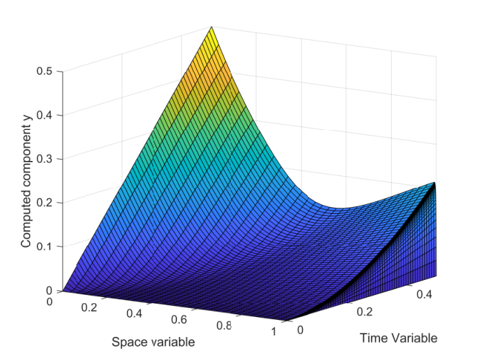
Note that a′​(0)=0a^{\prime}(0)=0 and A1=1≠0A_{1}=1\neq 0 in this example. In Figure 1 the computed component YY with the scheme (17) for ε=2−10\varepsilon=2^{-10} and N=M=64N=M=64 is shown. The approximation UU to the solution of Example 1 also appears in that figure; the interior layer emanating from the point (0,0)(0,0) and the boundary layer in the outflow boundary are observed. The numerical results are in Table 1 and they indicate that the numerical method (17) converges uniformly and globally with order O(N−1/2)O(N^{-1/2}) in agreement with Theorem 3.

Refer to caption
(a) Computed component YY
Refer to caption
(b) Numerical approximation UU
Figure 1: Example 1 with ε=2−10\varepsilon=2^{-10}: Computed component YY with the scheme (17) for N=M=64N=M=64 and the numerical approximation UU.
Table 1: Maximum two-mesh global differences and orders of convergence for Example 1
N=M=16 N=M=32 N=M=64 N=M=128 N=M=256 N=M=512 N=M=1024
ε=20\varepsilon=2^{0} 2.593E-03 1.306E-03 6.567E-04 3.285E-04 1.643E-04 8.212E-05 4.106E-05
0.989 0.992 1.000 1.000 1.000 1.000
ε=2−6\varepsilon=2^{-6} 3.004E-02 1.768E-02 1.014E-02 5.522E-03 2.888E-03 1.467E-03 7.321E-04
0.764 0.802 0.877 0.935 0.977 1.003
ε=2−12\varepsilon=2^{-12} 3.547E-02 2.356E-02 1.598E-02 1.103E-02 7.581E-03 5.175E-03 3.442E-03
0.590 0.560 0.535 0.541 0.551 0.588
ε=2−18\varepsilon=2^{-18} 3.551E-02 2.363E-02 1.609E-02 1.118E-02 7.818E-03 5.502E-03 3.877E-03
0.588 0.554 0.526 0.516 0.507 0.505
ε=2−24\varepsilon=2^{-24} 3.551E-02 2.363E-02 1.609E-02 1.118E-02 7.820E-03 5.505E-03 3.882E-03
0.588 0.554 0.525 0.516 0.506 0.504
ε=2−30\varepsilon=2^{-30} 3.551E-02 2.363E-02 1.609E-02 1.118E-02 7.820E-03 5.506E-03 3.882E-03
0.588 0.554 0.525 0.516 0.506 0.504
DN,MD^{N,M} 3.551E-02 2.363E-02 1.609E-02 1.118E-02 7.820E-03 5.506E-03 3.882E-03
PN,MP^{N,M} 0.588 0.554 0.525 0.516 0.506 0.504
Example 2.

Consider the example

ut−ε​ux​x+(1−t2)​ux=2​t​x,(x,t)∈(0,1)×(0,0.5],\displaystyle u_{t}-\varepsilon u_{xx}+(1-t^{2})u_{x}=2tx,\quad(x,t)\in(0,1)\times(0,0.5],
u⁡(x,0)=x3,x∈(0,1),\displaystyle u(x,0)=x^{3},\quad x\in(0,1),
u⁡(0,t)=1+t2,u⁡(1,t)=1,t∈[0,0.5].\displaystyle u(0,t)=1+t^{2},\ u(1,t)=1,\quad t\in[0,0.5].

In this example the data problem satisfy that a′​(0)=0a^{\prime}(0)=0 but A1=0A_{1}=0. The numerical results obtained for Example 2 with the numerical method (17) are given in Table 2 and they indicate that the method converges with almost first order as stated in Theorem 3.

Table 2: Maximum two-mesh global differences and orders of convergence for Example 2
N=M=16 N=M=32 N=M=64 N=M=128 N=M=256 N=M=512 N=M=1024
ε=20\varepsilon=2^{0} 6.959E-03 3.209E-03 1.541E-03 7.536E-04 3.725E-04 1.852E-04 9.233E-05
1.117 1.058 1.032 1.016 1.008 1.004
ε=2−6\varepsilon=2^{-6} 5.202E-02 2.956E-02 1.666E-02 9.232E-03 5.067E-03 2.751E-03 1.484E-03
0.816 0.827 0.852 0.865 0.881 0.891
ε=2−12\varepsilon=2^{-12} 6.938E-02 3.622E-02 2.037E-02 1.125E-02 6.138E-03 3.329E-03 1.792E-03
0.938 0.830 0.856 0.875 0.883 0.894
ε=2−18\varepsilon=2^{-18} 6.968E-02 3.634E-02 2.044E-02 1.130E-02 6.161E-03 3.342E-03 1.799E-03
0.939 0.830 0.855 0.875 0.882 0.894
ε=2−24\varepsilon=2^{-24} 6.969E-02 3.634E-02 2.044E-02 1.130E-02 6.162E-03 3.343E-03 1.799E-03
0.939 0.830 0.855 0.875 0.882 0.894
ε=2−30\varepsilon=2^{-30} 6.969E-02 3.634E-02 2.044E-02 1.130E-02 6.163E-03 3.340E-03 1.802E-03
0.939 0.830 0.855 0.874 0.884 0.890
DN,MD^{N,M} 6.969E-02 3.634E-02 2.044E-02 1.130E-02 6.163E-03 3.343E-03 1.802E-03
PN,MP^{N,M} 0.939 0.830 0.855 0.874 0.883 0.891
Example 3.

Consider the example

ut−ε​ux​x+(1+3​t2−2​t)​ux=4​x​(1−x),(x,t)∈(0,1)×(0,1.5],\displaystyle u_{t}-\varepsilon u_{xx}+(1+3t^{2}-2t)u_{x}=4x(1-x),\quad(x,t)\in(0,1)\times(0,1.5],
u⁡(x,0)=x3,x∈(0,1),\displaystyle u(x,0)=x^{3},\quad x\in(0,1),
u⁡(0,t)=1+0.25​t2,u⁡(1,t)=1,t∈[0,1.5].\displaystyle u(0,t)=1+0.25t^{2},\ u(1,t)=1,\quad t\in[0,1.5].

Note that a′​(0)≠0,A1=0a^{\prime}(0)\neq 0,A_{1}=0 and (1d) is not satisfied; then the interior and boundary layers interact with each other. This effect is observed in Figure 2 where the approximations to the component yy and the solution uu are shown. The numerical results obtained with the scheme (17) combined with a modification to the mesh in time [6, (19)] (see also Remark 1) are given in Table 3. These results suggest that the method converges globally and uniformly with almost first order.

Refer to caption
(a) Computed component YY
Refer to caption
(b) Numerical approximation UU
Figure 2: Example 3 with ε=2−10\varepsilon=2^{-10}: Computed component YY with the scheme (17) for N=M=64N=M=64 and the numerical approximation UU.
Table 3: Maximum two-mesh global differences and orders of convergence for Example 3
N=M=16 N=M=32 N=M=64 N=M=128 N=M=256 N=M=512 N=M=1024
ε=20\varepsilon=2^{0} 7.807E-02 3.389E-02 1.726E-02 8.507E-03 4.241E-03 2.117E-03 1.057E-03
1.204 0.973 1.021 1.004 1.002 1.002
ε=2−6\varepsilon=2^{-6} 1.042E-01 8.151E-02 5.318E-02 2.894E-02 1.705E-02 1.018E-02 5.732E-03
0.355 0.616 0.878 0.764 0.744 0.828
ε=2−12\varepsilon=2^{-12} 1.029E-01 8.090E-02 5.303E-02 2.889E-02 1.702E-02 1.017E-02 5.728E-03
0.347 0.609 0.876 0.763 0.743 0.828
ε=2−18\varepsilon=2^{-18} 1.025E-01 8.057E-02 5.295E-02 2.887E-02 1.747E-02 1.052E-02 5.982E-03
0.347 0.606 0.875 0.725 0.732 0.814
ε=2−24\varepsilon=2^{-24} 1.025E-01 8.052E-02 5.293E-02 2.886E-02 1.804E-02 1.094E-02 6.275E-03
0.348 0.605 0.875 0.678 0.721 0.802
ε=2−30\varepsilon=2^{-30} 1.025E-01 8.052E-02 5.293E-02 2.884E-02 1.813E-02 1.100E-02 6.326E-03
0.348 0.605 0.876 0.670 0.721 0.798
DN,MD^{N,M} 1.062E-01 8.509E-02 5.623E-02 2.897E-02 1.813E-02 1.100E-02 6.326E-03
PN,MP^{N,M} 0.319 0.598 0.957 0.676 0.721 0.798
Example 4.

Consider the example

ut−ε​ux​x+(1+x2)​ux=4​x​(1−x),(x,t)∈(0,1)×(0,0.5],\displaystyle u_{t}-\varepsilon u_{xx}+(1+x^{2})u_{x}=4x(1-x),\quad(x,t)\in(0,1)\times(0,0.5],
u⁡(x,0)=0,x∈(0,1),\displaystyle u(x,0)=0,\quad x\in(0,1),
u⁡(0,t)=u⁡(1,t)=t2,t∈[0,0.5].\displaystyle u(0,t)=u(1,t)=t^{2},\ \quad t\in[0,0.5].

Note that ax​(0,0)=0a_{x}(0,0)=0 and A0=A1=0A_{0}=A_{1}=0. The numerical results obtained with the scheme (17) are given in Table 4 and they indicate that the method converges with almost first order as stated in Theorem 4.

Table 4: Maximum two-mesh global differences and orders of convergence for Example 4
N=M=16 N=M=32 N=M=64 N=M=128 N=M=256 N=M=512 N=M=1024
ε=20\varepsilon=2^{0} 2.960E-03 1.515E-03 7.615E-04 3.819E-04 1.912E-04 9.567E-05 4.785E-05
0.967 0.992 0.996 0.998 0.999 1.000
ε=2−6\varepsilon=2^{-6} 2.590E-02 1.643E-02 9.829E-03 5.503E-03 3.026E-03 1.634E-03 8.757E-04
0.656 0.742 0.837 0.863 0.889 0.900
ε=2−12\varepsilon=2^{-12} 3.115E-02 2.004E-02 1.201E-02 6.698E-03 3.677E-03 1.992E-03 1.070E-03
0.636 0.739 0.843 0.865 0.884 0.897
ε=2−18\varepsilon=2^{-18} 3.126E-02 2.011E-02 1.205E-02 6.718E-03 3.689E-03 1.999E-03 1.073E-03
0.637 0.739 0.843 0.865 0.884 0.897
ε=2−24\varepsilon=2^{-24} 3.126E-02 2.011E-02 1.205E-02 6.719E-03 3.689E-03 1.999E-03 1.073E-03
0.637 0.739 0.843 0.865 0.884 0.897
ε=2−30\varepsilon=2^{-30} 3.126E-02 2.011E-02 1.205E-02 6.718E-03 3.690E-03 1.998E-03 1.075E-03
0.637 0.739 0.843 0.865 0.885 0.894
DN,MD^{N,M} 3.126E-02 2.011E-02 1.205E-02 6.719E-03 3.690E-03 1.999E-03 1.075E-03
PN,MP^{N,M} 0.637 0.739 0.843 0.865 0.884 0.895
Example 5.

Consider the example

ut−ε​ux​x+(1+x)​ux=4​x​(1−x),(x,t)∈(0,1)×(0,0.5],\displaystyle u_{t}-\varepsilon u_{xx}+(1+x)u_{x}=4x(1-x),\quad(x,t)\in(0,1)\times(0,0.5],
u⁡(x,0)=0,x∈(0,1),\displaystyle u(x,0)=0,\quad x\in(0,1),
u⁡(0,t)=t;u⁡(1,t)=t2,t∈[0,0.5].\displaystyle u(0,t)=t;\ u(1,t)=t^{2},\ \quad t\in[0,0.5].

Note that ax​(0,0)≠0a_{x}(0,0)\neq 0 and A0=0,A1≠0A_{0}=0,A_{1}\neq 0. The numerical results obtained with the scheme (17) are given in Table 5. They suggest that the method converges globally and uniformly with order O(N−1/2)O(N^{-1/2}), but the theoretical justification of these results remains open, as the proof in Theorem 4 requires ax​(0,0)=0a_{x}(0,0)=0.

Table 5: Maximum two-mesh global differences and orders of convergence for Example 5
N=M=16 N=M=32 N=M=64 N=M=128 N=M=256 N=M=512 N=M=1024
ε=20\varepsilon=2^{0} 1.426E-03 8.292E-04 4.557E-04 2.388E-04 1.222E-04 6.173E-05 3.099E-05
0.782 0.863 0.932 0.967 0.985 0.994
ε=2−6\varepsilon=2^{-6} 2.563E-02 1.562E-02 9.145E-03 5.113E-03 2.896E-03 1.600E-03 8.695E-04
0.714 0.772 0.839 0.820 0.856 0.879
ε=2−12\varepsilon=2^{-12} 3.099E-02 2.117E-02 1.437E-02 9.917E-03 6.914E-03 4.794E-03 3.258E-03
0.550 0.559 0.535 0.520 0.528 0.557
ε=2−18\varepsilon=2^{-18} 3.108E-02 2.128E-02 1.449E-02 1.007E-02 7.115E-03 5.061E-03 3.603E-03
0.547 0.554 0.525 0.501 0.492 0.490
ε=2−24\varepsilon=2^{-24} 3.108E-02 2.128E-02 1.449E-02 1.007E-02 7.119E-03 5.065E-03 3.609E-03
0.547 0.554 0.525 0.501 0.491 0.489
ε=2−30\varepsilon=2^{-30} 3.108E-02 2.128E-02 1.449E-02 1.007E-02 7.119E-03 5.065E-03 3.609E-03
0.547 0.554 0.525 0.501 0.491 0.489
DN,MD^{N,M} 3.108E-02 2.128E-02 1.449E-02 1.007E-02 7.119E-03 5.065E-03 3.609E-03
PN,MP^{N,M} 0.547 0.554 0.525 0.501 0.491 0.489
Remark 2.

In the numerical experiments performed, we have considered (27) when evaluating ψ0+\psi_{0}^{+} and θ:=d⁡(tj)​xi/(tj​ε)\theta:=d(t_{j})x_{i}/(t_{j}\varepsilon) is a large number with (xi,tj)∈GN,M(x_{i},t_{j})\in G^{N,M} to prevent overflow problems. If θ≥300\theta\geq 300, the value of the Mill’s ratio HH in Examples 1, 2 and 3 has been computed by using that

H⁡(r)∼1r​π​(1+∑m=1∞(−1)m​1.3​…​(2​m−1)(2​r2)m), as ​r→∞.H(r)\sim\frac{1}{r\sqrt{\pi}}\left(1+\sum_{m=1}^{\infty}(-1)^{m}\frac{1.3\ldots(2m-1)}{(2r^{2})^{m}}\right),\text{ as }r\to\infty.

This series has been approximated by the nn-th partial sum and the maximum two-mesh global differences in Tables 1,  2 and  3 have been obtained with n=5.n=5. Similar results have been obtained if larger values of nn are considered.

References

  • [1] Y. Amirat and A. Münch, Asymptotic analysis of an advection-diffusion equation involving interacting boundary and internal layers, Math. Methods Appl. Sci., v. 43 (11), (2020), 6823–6860.
  • [2] L. Bobisud, Second order linear parabolic equations with a small parameter, Arch. Rat. Mech,. Anal., v. 27, (1968), 385–397.
  • [3] P.A. Farrell, A.F. Hegarty, J.J.H. Miller, E. O’Riordan and G.I. Shishkin, Robust computational techniques for boundary layers, CRC Press, 2000.
  • [4] P. A. Farrell, A. F. Hegarty, J. J. H. Miller, E. O’ Riordan and G. I. Shishkin, Singularly perturbed convection diffusion problems with boundary and weak interior layers, J. Comput. Appl. Math., 2004, v. 166, n. 1, 133–151.
  • [5] A. Friedman, Partial differential equations of parabolic type, Prentice-Hall, Englewood Cliffs, N.J., 1964.
  • [6] J.L. Gracia and E. O’Riordan, Numerical approximations to a singularly perturbed convection-diffusion problem with a discontinuous initial condition, Numer. Algorithms, vol. 88 (4), 1851–1873, (2021).
  • [7] J.L. Gracia and E. O’Riordan, Parameter-uniform approximations for a singularly perturbed convection-diffusion problem with a discontinuous initial condition, Appl. Numer. Math., vol. 162, 106–123, (2021).
  • [8] J.L. Gracia and E. O’Riordan, Numerical approximation of solution derivatives of singularly perturbed parabolic problems of convection–diffusion type, Math. Comput., vol. 85, 2016, 581–599.
  • [9] O.A. Ladyzhenskaya, V.A. Solonnikov and N.N. Ural’tseva, Linear and quasilinear equations of parabolic type, Transactions of Mathematical Monographs, 23, American Mathematical Society, 1968.
  • [10] F.G. Lether, An elementary approximation for exp(x2x^{2})erfc(xx), J. Guant. Spectrosc. Radiant. Transfer, v. 43 (6), (1990), 511–513.
  • [11] T. Linß  and M. Stynes, Asymptotic analysis and Shishkin-type decomposition for an elliptic convection-diffusion problem. J. Math. Anal. Appl. 261 (2) 604–632, 2001.
  • [12] J.J.H. Miller, E. O’Riordan and G.I. Shishkin and L.P. Shishkina, Fitted mesh methods for problems with parabolic boundary layers, Mathematical Proceedings of the Royal Irish Academy, v. 98A, (1998), 173–190.
  • [13] J.J.H. Miller, E. O’Riordan and G.I. Shishkin, Fitted Numerical Methods for Singular Perturbation Problems, World-Scientific, Singapore (Revised edition), 2012.
  • [14] NIST Digital Library of Mathematical Functions. http://dlmf.nist.gov/, Release 1.1.6 of 2022–06–30. F. W. J. Olver, A. B. Olde Daalhuis, D. W. Lozier, B. I. Schneider, R. F. Boisvert, C. W. Clark, B. R. Miller, B. V. Saunders, H. S. Cohl, and M. A. McClain, eds.
  • [15] E. Pérez Sinusia, Asymptotic approximations for singularly perturbed convection-diffusion problems with discontinuous boundary data, Ph. D. thesis, Univeridad Publica de Navarra, Pamplona, Spain, (2005).
  • [16] S. D. Shih, On a class of singularly perturbed parabolic equations, ZAMM Z. Angew. Math. Mech., v. 81 (5), (2001), 337–345.

6 Appendix: Bounds on the partial derivatives of the functions ψi±​(x,t)\psi^{\pm}_{i}(x,t).

The functions ψi±​(x,t)\psi^{\pm}_{i}(x,t) are defined by means of the iterated integrals of the complementary error function. Define

erfc−1⁡(x):=2π​e−x2,erfcn⁡(x):=∫s=x∞erfcn−1⁡(s)​𝑑s,n≥0.\erfc_{-1}(x):=\frac{2}{\sqrt{\pi}}e^{-x^{2}},\quad\erfc_{n}(x):=\int_{s=x}^{\infty}\erfc_{n-1}(s)\,ds,\quad n\geq 0.

Note that erfc0⁡(x)=erfc⁡(x)\erfc_{0}(x)=\erfc(x) 44 4 The first three iterated integrals of the complementary error function are erfc1⁡(x)\displaystyle\erfc_{1}(x) =e−x2π−x​erfc⁡(x)=e−x2​(1π−x​ex2​erfc⁡(x)),\displaystyle=\frac{e^{-x^{2}}}{\sqrt{\pi}}-x\erfc(x)=e^{-x^{2}}\left(\frac{1}{\sqrt{\pi}}-xe^{x^{2}}\erfc(x)\right), erfc2⁡(x)\displaystyle\erfc_{2}(x) =14​((1+2​x2)​erfc⁡(x)−2​x​e−x2π),\displaystyle=\frac{1}{4}\left((1+2x^{2})\erfc(x)-\frac{2xe^{-x^{2}}}{\sqrt{\pi}}\right), erfc3⁡(x)\displaystyle\erfc_{3}(x) =16​((1+x2)​e−x2π−(3​x+2​x3)2​erfc⁡(x)).\displaystyle=\frac{1}{6}\left(\frac{(1+x^{2})e^{-x^{2}}}{\sqrt{\pi}}-\frac{(3x+2x^{3})}{2}\erfc(x)\right). and

erfcn⁡(x)=2π​∫s=x∞(s−x)nn!​e−s2​𝑑s.\erfc_{n}(x)=\frac{2}{\sqrt{\pi}}\int_{s=x}^{\infty}\frac{(s-x)^{n}}{n!}e^{-s^{2}}ds.

In addition, we have the following identities [14]

n​erfcn⁡(x)+x​erfcn−1⁡(x)\displaystyle n\erfc_{n}(x)+x\erfc_{n-1}(x) =12​erfcn−2⁡(x);n≥1;\displaystyle=\frac{1}{2}\erfc_{n-2}(x);\quad n\geq 1; (22a)
(−1)n​erfcn⁡(x)+erfcn⁡(−x)\displaystyle(-1)^{n}\erfc_{n}(x)+\erfc_{n}(-x) =i−n2n−1​n!​Hn​(i​x);n≥0,\displaystyle=\frac{i^{-n}}{2^{n-1}n!}H_{n}(ix);\quad n\geq 0, (22b)

where i2=−1i^{2}=-1 and HnH_{n} is the Hermite polynomial of degree nn. Recall the definitions in (4) and note that

ψ1±​(x,t)\displaystyle\psi^{\pm}_{1}(x,t) =(x±d⁡(t))​ψ0±​(x,t)+2​ε​t​ψ−1±​(x,t),\displaystyle=(x\pm d(t))\psi_{0}^{\pm}(x,t)+2\varepsilon t\psi_{-1}^{\pm}(x,t),\ (23a)
2​t​∂ψ1−∂t\displaystyle 2t\frac{\partial\psi^{-}_{1}}{\partial t} =ψ1−−(2​t​a​(d⁡(t),t)+(x−d⁡(t)))​ψ0−,\displaystyle=\psi^{-}_{1}-\bigl(2ta(d(t),t)+(x-d(t))\bigr)\psi^{-}_{0}, (23b)
2​t​∂ψ1+∂t\displaystyle 2t\frac{\partial\psi_{1}^{+}}{\partial t} =(1+2​x​p​(t)ε​t)​ψ1++(2​t​a​(d⁡(t),t)−(x+d⁡(t)))​ψ0+,\displaystyle=\left(1+\frac{2xp(t)}{\varepsilon t}\right)\psi_{1}^{+}+\bigl(2ta(d(t),t)-(x+d(t))\bigr)\psi_{0}^{+}, (23c)
where
OPENp⁡(t):=t​a​(d⁡(t),t)−d⁡(t)=∫s=0ta⁡(d⁡(t),t)−a⁡(d⁡(s),s))​𝑑s.p(t):=ta(d(t),t)-d(t)=\int_{s=0}^{t}a(d(t),t)-a(d(s),s))\ ds. (23d)

Observe that p⁡(t)≡0p(t)\equiv 0, when a⁡(x,t)=aa(x,t)=a is a constant.

Some recurrence relations are given below which are useful when bounding the derivatives of the functions ψn±​(x,t)\psi^{\pm}_{n}(x,t).

For all n≥1n\geq 1
∂ψn−∂x=n​ψn−1−,∂ψn+∂x=n​ψn−1++d⁡(t)ε​t​ψn+,\frac{\partial\psi^{-}_{n}}{\partial x}=n\psi^{-}_{n-1},\quad\frac{\partial\psi^{+}_{n}}{\partial x}=n\psi^{+}_{n-1}+\frac{d(t)}{\varepsilon t}\psi_{n}^{+}, (24a)
and for all n≥2n\geq 2 (using (22a)) we have
ψn±​(x,t)\displaystyle\psi^{\pm}_{n}(x,t) =(x±d⁡(t))​ψn−1±​(x,t)+2​(n−1)​ε​t​ψn−2±​(x,t),\displaystyle=(x\pm d(t))\psi_{n-1}^{\pm}(x,t)+2(n-1)\varepsilon t\psi_{n-2}^{\pm}(x,t), (24b)
∂ψn−∂t\displaystyle\frac{\partial\psi^{-}_{n}}{\partial t} =ε​n​(n−1)​ψn−2−−a⁡(d⁡(t),t)​n​ψn−1−,\displaystyle=\varepsilon n(n-1)\psi^{-}_{n-2}-a(d(t),t)n\psi^{-}_{n-1},
∂ψn+∂t\displaystyle\frac{\partial\psi^{+}_{n}}{\partial t} =ε​n​(n−1)​ψn−2++(2​d⁡(t)t−a⁡(d⁡(t),t))​n​ψn−1+\displaystyle=\varepsilon n(n-1)\psi^{+}_{n-2}+\left(2\frac{d(t)}{t}-a(d(t),t)\right)n\psi^{+}_{n-1}
−p⁡(t)ε​t2​(d⁡(t)​ψn+−ψn+1+).\displaystyle-\frac{p(t)}{\varepsilon t^{2}}(d(t)\psi^{+}_{n}-\psi^{+}_{n+1}).

In the case of constant coefficients one has L​ψn−=L​ψn+=0L\psi^{-}_{n}=L\psi^{+}_{n}=0, but for variable a⁡(x,t)a(x,t), by using (22a) we have that for all n≥0n\geq 0

L​ψn−\displaystyle L\psi^{-}_{n} =(a⁡(d⁡(t),t)−a⁡(x,t))​∂ψn−∂x,\displaystyle=(a(d(t),t)-a(x,t))\frac{\partial\psi^{-}_{n}}{\partial x}, (25a)
L​ψn+\displaystyle L\psi^{+}_{n} =(a⁡(d⁡(t),t)−a⁡(x,t))​∂ψn+∂x+p⁡(t)​ψn+1+ε​t2.\displaystyle=(a(d(t),t)-a(x,t))\frac{\partial\psi^{+}_{n}}{\partial x}+p(t)\frac{\psi^{+}_{n+1}}{\varepsilon t^{2}}. (25b)

Using the inequality erfc⁡(z)≤C​e−z2≤C​eγ2/4​e−γ​z,∀z≥0\erfc(z)\leq Ce^{-z^{2}}\leq Ce^{\gamma^{2}/4}e^{-\gamma z},\forall z\geq 0 it follows (see [6] and [7]) that

|∂j∂tj​ψ0−​(x,t)|,|∂j∂tj​E​(x,t)|≤C​(1t+1ε​t)j​Eγ​(x,t);j=1,2,\displaystyle\left|\frac{\partial^{j}}{\partial t^{j}}\psi^{-}_{0}(x,t)\right|,\left|\frac{\partial^{j}}{\partial t^{j}}E(x,t)\right|\leq C\left(\frac{1}{t}+\frac{1}{\sqrt{\varepsilon t}}\right)^{j}E_{\gamma}(x,t);\quad j=1,2, (26a)
|ψ0−​(x,t)|≤Cand|ψ0−​(x,t)|≤C​E​(x,t),ifx≥d⁡(t),\displaystyle\left|\psi^{-}_{0}(x,t)\right|\leq C\quad\hbox{and}\quad|\psi^{-}_{0}(x,t)|\leq CE(x,t),\quad\hbox{if}\quad x\geq d(t), (26b)
|∂i∂xi​ψ0−​(x,t)|,|∂i∂xi​E​(x,t)|≤C​(1ε​t)i​Eγ​(x,t),1≤i≤4.\displaystyle\left|\frac{\partial^{i}}{\partial x^{i}}\psi^{-}_{0}(x,t)\right|,\left|\frac{\partial^{i}}{\partial x^{i}}E(x,t)\right|\leq C\left(\frac{1}{\sqrt{\varepsilon t}}\right)^{i}E_{\gamma}(x,t),\quad 1\leq i\leq 4. (26c)

The following remark is used to prove bounds on the derivatives of the singular function ψ0+\psi^{+}_{0} and to compute the numerical results presented in Section §5 (see Remark 2).

Remark 3.

The function ψ0+\psi^{+}_{0} can be written as

ψ0+​(x,t)=12​ed⁡(t)​xt​ε​erfc⁡(x+d⁡(t)2​ε​t)=12​E​(x,t)​H​(x+d⁡(t)2​ε​t),\psi^{+}_{0}(x,t)=\frac{1}{2}e^{\frac{d(t)x}{t\varepsilon}}\erfc\left(\frac{x+d(t)}{2\sqrt{\varepsilon t}}\right)=\frac{1}{2}E(x,t)\,H\left(\frac{x+d(t)}{2\sqrt{\varepsilon t}}\right), (27)

where HH is the Mill’s ratio and it is defined by H⁡(x):=ex2​erfc⁡(x).H(x):=e^{x^{2}}\erfc(x). From [10], we have the inequality

1π−1π​x+1+x2π≤H⁡(x)≤12π​x+1+(π−2)2​x2π.\frac{1}{\frac{\pi-1}{\sqrt{\pi}}x+\sqrt{1+\frac{x^{2}}{\pi}}}\leq H(x)\leq\frac{1}{\frac{2}{\sqrt{\pi}}x+\sqrt{1+\frac{(\pi-2)^{2}x^{2}}{\pi}}}. (28)

Hence, for all x>0x>0

(1−π​x​H​(x))≤min⁡{12​x2,1π​x},\left(1-\sqrt{\pi}xH(x)\right)\leq\min\left\{\frac{1}{2x^{2}},\frac{1}{\sqrt{\pi}x}\right\},

and

ed⁡(t)​xt​ε​erfc1⁡(x+d⁡(t)2​ε​t)=E⁡(x,t)π​(1−π​(x+d⁡(t)2​ε​t)​H​(x+d⁡(t)2​ε​t)).e^{\frac{d(t)x}{t\varepsilon}}\erfc_{1}\left(\frac{x+d(t)}{2\sqrt{\varepsilon t}}\right)=\frac{E(x,t)}{\sqrt{\pi}}\left(1-\sqrt{\pi}\left(\frac{x+d(t)}{2\sqrt{\varepsilon t}}\right)H\left(\frac{x+d(t)}{2\sqrt{\varepsilon t}}\right)\right).

Hence,

1ε​t​(ed⁡(t)​xt​ε​erfc1⁡(x+d⁡(t)2​ε​t))≤C​E⁡(x,t)x+d⁡(t)​min⁡{1,ε​tx+d⁡(t)}.\frac{1}{\sqrt{\varepsilon t}}\left(e^{\frac{d(t)x}{t\varepsilon}}\erfc_{1}\left(\frac{x+d(t)}{2\sqrt{\varepsilon t}}\right)\right)\leq C\frac{E(x,t)}{x+d(t)}\min\left\{1,\frac{\sqrt{\varepsilon t}}{x+d(t)}\right\}. (29)

In the next lemma bounds on the derivatives of the function ψ0+\psi^{+}_{0} are deduced.

Lemma 2.

For the singular function ψ0+\psi^{+}_{0}, we have the following bounds

|ψ0+​(x,t)|\displaystyle|\psi^{+}_{0}(x,t)| ≤C​min⁡{1,ε​tx+d⁡(t)}​E​(x,t),\displaystyle\leq C\min\left\{1,\frac{\sqrt{\varepsilon t}}{x+d(t)}\right\}E(x,t), (30a)
|∂∂t​ψ0+​(x,t)|\displaystyle\left|\frac{\partial}{\partial t}\psi^{+}_{0}(x,t)\right| ≤Ct​Eγ​(x,t),\displaystyle\leq\frac{C}{t}E_{\gamma}(x,t), (30b)
|∂2∂t2​ψ0+​(x,t)|\displaystyle\left|\frac{\partial^{2}}{\partial t^{2}}\psi^{+}_{0}(x,t)\right| ≤Ct2​(1+tε)​Eγ​(x,t),\displaystyle\leq\frac{C}{t^{2}}\left(1+\sqrt{\frac{t}{\varepsilon}}\right)E_{\gamma}(x,t), (30c)
|∂∂x​ψ0+​(x,t)|\displaystyle\left|\frac{\partial}{\partial x}\psi^{+}_{0}(x,t)\right| ≤Cx+d⁡(t)​Eγ​(x,t),\displaystyle\leq\frac{C}{x+d(t)}E_{\gamma}(x,t), (30d)
|∂2∂x2​ψ0+​(x,t)|\displaystyle\left|\frac{\partial^{2}}{\partial x^{2}}\psi^{+}_{0}(x,t)\right| ≤Cε​t​Eγ​(x,t),\displaystyle\leq\frac{C}{\varepsilon t}E_{\gamma}(x,t), (30e)
|∂3∂x3​ψ0+​(x,t)|\displaystyle\left|\frac{\partial^{3}}{\partial x^{3}}\psi^{+}_{0}(x,t)\right| ≤Cε2​t​(1+εt)​Eγ​(x,t).\displaystyle\leq\frac{C}{\varepsilon^{2}t}\left(1+\sqrt{\frac{\varepsilon}{t}}\right)E_{\gamma}(x,t). (30f)
Proof.

Note first that

p⁡(t)=t​a​(d⁡(t),t)−d⁡(t)=∫s=0t∫r=d⁡(s)d⁡(t)ax​(r,t)​𝑑r​𝑑s+∫s=0t∫r=stat​(d⁡(s),r)​𝑑r​𝑑s.\displaystyle p(t)=ta(d(t),t)-d(t)=\int_{s=0}^{t}\int_{r=d(s)}^{d(t)}a_{x}(r,t)dr\,ds+\int_{s=0}^{t}\int_{r=s}^{t}a_{t}(d(s),r)dr\,ds.

Hence, |p⁡(t)|≤C​t2.|p(t)|\leq Ct^{2}.55 5 In the particular case of ∇a​(0,0)=(0,0)\nabla a(0,0)=(0,0), one has |p⁡(t)|≤C​t3|p(t)|\leq Ct^{3}. To prove (30a), we use that |H⁡(r)|≤C|H(r)|\leq C and r​H​(r)≤CrH(r)\leq C for all r≥0r\geq 0, where HH is defined in Remark 3. Then,

(x+d⁡(t))​ψ0+​(x,t)≤C​ε​t​E​(x,t)andψ0+​(x,t)≤C​E​(x,t).(x+d(t))\psi^{+}_{0}(x,t)\leq C\sqrt{\varepsilon t}E(x,t)\quad\hbox{and}\quad\psi^{+}_{0}(x,t)\leq CE(x,t).

Using (29), (30a) and the identity (24b) we easily establish the following bounds

|ψi+(x,t)|≤C(ε​t)imin{1,εt}E(x,t),i=1,2.\,|\psi^{+}_{i}(x,t)|\leq C(\sqrt{\varepsilon t})^{i}\min\left\{1,\sqrt{\frac{\varepsilon}{t}}\right\}E(x,t),\quad i=1,2. (31)

To prove (30b), observe that

(x+d⁡(t))​∂ψ0+​(x,t)∂t=x​p​(t)t​((x+d⁡(t))t​ε​ψ0+​(x,t)−E⁡(x,t)ε​π​t)\displaystyle(x+d(t))\frac{\partial\psi^{+}_{0}(x,t)}{\partial t}=\frac{xp(t)}{t}\left(\frac{(x+d(t))}{t\varepsilon}\psi^{+}_{0}(x,t)-\frac{E(x,t)}{\sqrt{\varepsilon\pi t}}\right)
+(4​x​p​(t)+(x+d⁡(t))​((x+d⁡(t)−2​t​a​(t)))​E⁡(x,t)4​t​ε​π​tCLOSE\displaystyle\hskip 28.45274pt+\left(4xp(t)+(x+d(t))((x+d(t)-2ta(t))\right)\frac{E(x,t)}{4t\sqrt{\varepsilon\pi t}}
=x​p​(t)ε​t2​ψ1+​(x,t)+(x−d⁡(t))2​E⁡(x,t)4​t​ε​π​t+a⁡(d⁡(t),t)​(x−d⁡(t))​E⁡(x,t)2​ε​π​t,\displaystyle\hskip 28.45274pt=\frac{xp(t)}{\varepsilon t^{2}}\psi^{+}_{1}(x,t)+(x-d(t))^{2}\frac{E(x,t)}{4t\sqrt{\varepsilon\pi t}}+a(d(t),t)(x-d(t))\frac{E(x,t)}{2\sqrt{\varepsilon\pi t}},

and use (29) and |p⁡(t)|≤C​t2|p(t)|\leq Ct^{2}. Next, we prove (30c). We have that

(x+d⁡(t))​∂2ψ0+​(x,t)∂t2\displaystyle(x+d(t))\frac{\partial^{2}\psi^{+}_{0}(x,t)}{\partial t^{2}} =∂∂t​(x​p​(t)ε​t2​ψ1+​(x,t)+(x+d⁡(t)+2​p​(t))​(x−d⁡(t))​E​(x,t)4​t​ε​π​t)\displaystyle=\frac{\partial}{\partial t}\Bigl(\frac{xp(t)}{\varepsilon t^{2}}\psi^{+}_{1}(x,t)+(x+d(t)+2p(t))\frac{(x-d(t))E(x,t)}{4t\sqrt{\varepsilon\pi t}}\Bigr)
−a⁡(d⁡(t),t)​∂ψ0+​(x,t)∂t\displaystyle-a(d(t),t)\frac{\partial\psi^{+}_{0}(x,t)}{\partial t}
and |∂∂t​(p⁡(t)t2)|≤C+C​‖∇a​(0,0)‖t≤Ct,\displaystyle\left|\frac{\partial}{\partial t}\left(\frac{p(t)}{t^{2}}\right)\right|\leq C+C\frac{\|\nabla a(0,0)\|}{t}\leq\frac{C}{t},
|(x−d⁡(t))2​ε​t​∂E⁡(x,t)∂t|≤Ct​(1+tε)​Eγ​(x,t),\displaystyle\left|\frac{(x-d(t))}{2\sqrt{\varepsilon t}}\frac{\partial E(x,t)}{\partial t}\right|\leq\frac{C}{t}\left(1+\sqrt{\frac{t}{\varepsilon}}\right)E_{\gamma}(x,t),
|ψ1+​(x,t)ε​t|≤Ct​min⁡{1,tε}​Eγ​(x,t),\displaystyle\left|\frac{\psi^{+}_{1}(x,t)}{\varepsilon t}\right|\leq\frac{C}{t}\min\left\{1,\sqrt{\frac{t}{\varepsilon}}\right\}E_{\gamma}(x,t),
∂ψ1+​(x,t)∂t=(12​t+x​p​(t)ε​t2)​ψ1+​(x,t)+2​p​(t)−(x−d⁡(t))2​t​ψ0+​(x,t).\displaystyle\frac{\partial\psi_{1}^{+}(x,t)}{\partial t}=\left(\frac{1}{2t}+\frac{xp(t)}{\varepsilon t^{2}}\right)\psi_{1}^{+}(x,t)+\frac{2p(t)-(x-d(t))}{2t}\psi_{0}^{+}(x,t).

Collecting all of these bounds yields (30c). From

(x+d⁡(t))​∂∂x​ψ0+​(x,t)=d⁡(t)​(x+d⁡(t)t​ε​ψ0+​(x,t)−E⁡(x,t)ε​π​t)−(x−d⁡(t))​E​(x,t)2​ε​π​t,(x+d(t))\frac{\partial}{\partial x}\psi^{+}_{0}(x,t)=d(t)\left(\frac{x+d(t)}{t\varepsilon}\psi^{+}_{0}(x,t)-\frac{E(x,t)}{\sqrt{\varepsilon\pi t}}\right)-\frac{(x-d(t))E(x,t)}{2\sqrt{\varepsilon\pi t}},

and (29), we have  (30d). Note also that for i=2,3i=2,3

∂i∂xi​ψ0+​(x,t)=d⁡(t)t​ε​∂i−1∂xi−1​ψ0+​(x,t)−12​ε​π​t​∂i−1∂xi−1​E​(x,t),\frac{\partial^{i}}{\partial x^{i}}\psi^{+}_{0}(x,t)=\frac{d(t)}{t\varepsilon}\frac{\partial^{i-1}}{\partial x^{i-1}}\psi^{+}_{0}(x,t)-\frac{1}{2\sqrt{\varepsilon\pi t}}\frac{\partial^{i-1}}{\partial x^{i-1}}E(x,t),

from which (30e) and (30f) follows. ∎