Equation of state of hard-disk fluids under single-file confinement

We consider a system of $N$ hard disks of unit diameter confined in a long channel of length $L\gg 1$ and width $w=1+\epsilon$, with $0\leq\epsilon\leq\epsilon_{\mathrm{max}}$, where $\epsilon_{\mathrm{max}}=\sqrt{3}/2\simeq 0.866$ in order to ensure the single-file condition and preclude second nearest-neighbor interactions, as depicted in Fig. 1(a). As illustrated in Fig. 1(b), if the transverse separation between two disks at contact is $s$, their longitudinal separation is

The number of disks per unit area is $\rho=N/Lw$. However, in the Q1D configuration of the system, it is convenient to characterize the number density through the number of particles per unit length, $\lambda\equiv N/L=\rho w$. Its close-packing value (given an excess pore width $\epsilon$) is $\lambda_{\mathrm{cp}}(\epsilon)=1/a(\epsilon)$, as inferred from Fig. 1(b), at which the particles occupy the maximum available space, resulting in the pressure diverging at that value. This divergence will be discussed in depth in Sec. II.4. We note that $\lambda_{\text{cp}}(\epsilon_{\mathrm{max}})=2$.

Due to the anisotropy of the original 2D system, the transverse pressure ($P_{\perp}$) is different from the longitudinal one ($P_{\|})$. We, then, define the (reduced) Q1D pressure as $p\equiv P_{\|}w$, where, henceforth, we take $k_{B}T=1$ as unit energy ($k_{B}$ and $T$ being the Boltzmann constant and the absolute temperature, respectively).

The exact solution to the Q1D system can be obtained via the transfer-matrix method. In the thermodynamic limit of large $N$, the excess Gibbs free energy per particle, $g^{\text{ex}}(p)$, may be written asKofke and Post 1993

where $\ell(p)$ is the maximum eigenvalue corresponding to the problem

and $\phi(y)$ is the associated eigenfunction. Here and henceforth, all integrations over the $y$-variable will be understood to run along the interval $-\epsilon/2\leq y\leq\epsilon/2$ (where the origin $y=0$ is taken at the centerline) and the integration limits will be omitted. Under the normalization condition

$\phi^{2}(y)$ represents the probability density along the transverse direction $y$ within this framework. Multiplying both sides of Eq. (3) by $\phi(y_{1})$ and integrating over $y_{1}$, we obtain

where the normalization condition, Eq. (4), has been used.

Of course, both $\ell$ and $\phi(y)$ are functions of $p$. Differentiating both sides of Eq. (5) with respect to $p$, one obtains

On account of Eq. (3), the second term on the right-hand side of Eq. (II.2) can be rewritten as $2\ell\int\mathrm{d}y_{1}\,\phi(y_{1})\partial_{p}\phi(y_{1})=\ell\partial_{p}\int\mathrm{d}y_{1}\,\phi^{2}(y_{1})=0$. Thus, $\partial_{p}\ell$ is only given by the first term on the right-hand side of Eq. (II.2).

The compressibility factor $Z\equiv p/\lambda$ can be obtained from the Gibbs free energy by the thermodynamic relation $Z=1+p\partial_{p}g^{\text{ex}}(p)=1-(p/\ell)\partial_{p}\ell$. Making use of Eq. (II.2), one obtains

Taking into account Eq. (5), Eq. (7) can be rewritten as

It should be noted that, in contrast to the form (7), the eigenfunction $\phi(y)$ in the form (8) does not need to be normalized. While both forms are fully equivalent inasmuch as the exact $\ell$ and $\phi(y)$ are used, they differ in the case of approximations.

It is interesting to remark that the solution shown here can also be obtained by a mapping of the original Q1D system onto a 1D non-additive mixture of hard rods, as outlined in Appendix A.

It should be noted also that in the limit $\epsilon\to 0$ (at finite $p$), one obtains $\phi(y)\to\epsilon^{-1/2}\Theta(\frac{\epsilon}{2}-|y|)$, $\ell\to e^{-p}\epsilon$, $g^{\text{ex}}(p)\to p$, and $Z\to 1+p$ from Eqs. (3), (2), and (7), respectively, thus recovering the equation of state of the Tonks gas,Tonks 1936 as expected.

Virial expansions are one of the most common methods to describe fluids under low-density (or, equivalently, low-pressure) conditions.Hansen and McDonald 2013; Santos 2016 In general, access to the exact virial coefficients of a given system, at least the lower-order ones, is fundamental to improve the knowledge of the system and also to test the accuracy of approximate methods.

The virial coefficients $\{B_{n}\}$ are defined from the expansion of the compressibility factor in powers of density,

Analogously, one can introduce the expansion of $g^{\text{ex}}$ and $Z$ in powers of pressure,

where

and so on. The second virial coefficient has an analytical expression, namely,Kamenetskiy, Mon, and Percus 2004; Mon 2018

To the best of our knowledge, the correct third and fourth virial coefficients have not been evaluated yet. Here, we derive them from the exact transfer-matrix solution, Eq. (7), without assuming the direct application of the standard diagrammatic method.Mon 2014; Mon 2015; Mon 2020

Let us introduce the expansion in powers of $p$ of both the eigenvalue and the eigenfunction in Eq. (3) as

Inserting the expansion of $\ell$ into Eq. (2) and comparing with Eq. (10a), we obtain

where we have used $\ell_{0}=\epsilon$ and $\ell_{1}=-\epsilon B_{2}$ (see Appendix B). Alternatively, the expansion of $\phi(y)$ provides the expansion of the integral

Since $I=-\partial_{p}\ell$ [see Eq. (II.2)], one has

By inserting the series expansions of Eq. (13) into both the normalization condition, Eq. (4), and the eigenvalue equation, Eq. (3), and equating the coefficients with the same powers of $p$ on both sides of the equation, one can, in principle, obtain as many terms as desired. Appendix B shows the calculation of $\{\phi_{0},\phi_{1},\phi_{2}\}$ and $\{\ell_{0},\ell_{1},\ell_{2}\}$. In addition, $\ell_{3}$ can be obtained from $I_{2}$. Substitution of $\ell_{2}$ and $\ell_{3}$ into Eq. (14), yields

where $W_{2}$ and $W_{3}$ are given by Eqs. (B) and (B), requiring to numerically carry out a simple and double integration, respectively.

The exact expressions derived here for $B_{3}^{\prime}$ and $B_{4}^{\prime}$ turn out to differ from those (hereafter referred to as $B_{3,\text{irr}}^{\prime}$ and $B_{4,\text{irr}}^{\prime}$) obtained via the integration of standard irreducible diagrams.Mon 2014; Mon 2015; Mon 2020 In particular, the leading terms in the expansions in powers of $\epsilon$ of the latter coefficients are $B_{3,\text{irr}}^{\prime}=-\frac{\epsilon^{4}}{144}+\mathcal{O}(\epsilon^{6})$ and $B_{4,\text{irr}}^{\prime}=-\frac{\epsilon^{6}}{160}+\mathcal{O}(\epsilon^{8})$, which contrast with the leading terms in Eq. (17).

The origin of the discrepancy between the exact virial coefficients obtained here from the transfer-matrix solution, Eq. (7), and those derived from the standard diagrammatic schemeMon 2014; Mon 2015; Mon 2020 lies on the implicit assumption of a cancellation of the so-called reducible diagrams in the latter method. This cancellation is inherently associated with the factorization property of the reducible diagrams into products of irreducible ones,Santos 2016 as a consequence of the translational invariance of the position of any particle. While this factorization property holds in bulk fluids, it fails under confinement, due to the breakdown of the translational invariance along the confined directions.

Let us take the coefficient $B_{3}$ as the simplest example. By assuming cancellation of the reducible diagrams, one would have a single irreducible diagram, namely,Mon 2020

On the other hand, the actual result is

Here, the diagrams have its usual meaning,Santos 2016 except that they are supposed to be divided by $L\epsilon^{n}$, $n$ being the number of particles represented in the diagram. In a bulk fluid, $\Delta B_{3}=0$, due to the factorization property of the reducible diagrams mentioned before. However, in our confined system, one has

so that $\Delta B_{3}=4(B_{2}^{2}-W_{2})\neq 0$. As a by-product, from Eq. (17), we obtain

This is equivalent to but much more compact than the expression derived in Ref. Mon 2020.

It is worth mentioning that this issue regarding the correction needed to the irreducible-diagram representation of the virial coefficients arises also when dealing with flexible molecules.Caracciolo, Mognetti, and Pelissetto 2006

The performance of the virial series truncated after the fourth coefficient can be inspected by comparison with the exact equation of state.Kofke and Post 1993; Pergamenshchik 2020 The conventional truncated series from Eq. (9) would be $Z\to Z_{\text{tr}}(\lambda)\equiv 1+B_{2}\lambda+B_{3}\lambda^{2}+B_{4}\lambda^{3}$. Alternatively, with the same amount of information, one can truncate the series at the level of Eq. (10b) to obtain $Z\to Z_{\text{tr}}^{\prime}(p)\equiv 1+B_{2}p+B_{3}^{\prime}p^{2}+B_{4}^{\prime}p^{3}$, where the density dependence of the compressibility factor is defined in parametric form ($p$ being the parameter) by the pair $Z=Z_{\text{tr}}^{\prime}(p)$ and $\lambda=p/Z_{\text{tr}}^{\prime}(p)$. As Fig. 2 shows, the truncated series $Z_{\text{tr}}(\lambda)$ is reliable only for $\lambda\lesssim 0.4$, whereas the truncated series $Z_{\text{tr}}^{\prime}(p)$ is very accurate even at $\lambda\approx 1$, especially for small pore widths. This is not surprising given the fact that the exact equation of state for hard rods is $Z=1+B_{2}p$ (with $B_{2}=1$).Tonks 1936 On the other hand, neither $Z_{\text{tr}}(\lambda)$ nor $Z_{\text{tr}}^{\prime}(p)$ capture the divergence of pressure in the limit $\lambda\to\lambda_{\text{cp}}$ discussed in Sec. II.4.

Before turning to the high-pressure limit in Sec. II.4, let us draw two relevant points from the analysis in this section. First, if for a given confined fluid with an unknown exact solution one needs to resort to the virial coefficients (either analytically or numerically), then the standard irreducible diagrams do not provide the right answer. Instead, one would need to go back to the derivation stepsSantos 2016 and include the reducible diagrams as well, which fail to cancel if the translational invariance is broken down. Second, if the first few virial coefficients are known and a truncated equation of state is employed as an approximation, the recommendation is to employ the pressure representation,Maestre et al. 2011 Eq. (10b), rather than the density representation, Eq. (9).

Solving numerically the eigenvalue problem in Eq. (3) becomes increasingly more difficult as pressure grows and the system approaches the close-packing limit. It is, therefore, of interest to study analytically the limit $p\to\infty$ (or, equivalently, $\lambda\to\lambda_{\text{cp}}$) in order to understand the full behavior of the system.

In this high-pressure limit, particles accumulate more and more near the walls, which means that $\phi(y)$ becomes non-zero only in two symmetric layers near $y=\pm\frac{\epsilon}{2}$. As a consequence, the eigenfunction $\phi(y)$ and the eigenvalue $\ell$ for high values of $p$ adopt the forms (see Appendix C for details)

In Eq. (22a), the normalization constant is

It should be noted that, for high $p$, $\phi_{\pm}(y)$ is practically nonzero only inside a region of width of the order of $a(\epsilon)/\epsilon p$, adjacent to the wall at $y=\pm\frac{\epsilon}{2}$.

As proved in Appendix C, the high-pressure compressibility factor becomes

Table 1 shows that exact and MC simulation dataMon 2020 confirm the validity of Eq. (24) as pressure increases. Recalling that $\lambda_{\text{cp}}=1/a(\epsilon)$, Eq. (24) can be recast as

Equation (25) embodies two important features of the high-pressure asymptotic behavior of the compressibility factor. First, $Z$ presents a simple pole at $\lambda=\lambda_{\text{cp}}$, as expected. Second, the residue of the pole is not $1$ (as happens in the hard-rod Tonks gas,Tonks 1936) but $2$. These two features are made quite apparent in Fig. 3, where the exact normalized compressibility factor $(1-\lambda/\lambda_{\text{cp}})Z$ is plotted as a function of the scaled density $\lambda/\lambda_{\text{cp}}$ for several values of $\epsilon$. It can be observed that the normalized quantity $(1-\lambda/\lambda_{\text{cp}})Z$ starts growing with density, then reaches a peak at a certain value $\lambda_{\text{peak}}$, and subsequently decays toward its asymptotic value $2$. We have checked that $\lambda_{\text{peak}}$ is slightly higher than $1$ for any $\epsilon$, namely, $\lambda_{\text{peak}}\simeq 1+\frac{1}{10}\epsilon^{2}$. Thus, in the region of small pore width, one has $1-\lambda/\lambda_{\text{cp}}\approx\frac{2}{5}\epsilon^{2}$. It is then obvious that the limiting value $(1-\lambda/\lambda_{\text{cp}})Z\to 2$ requires linear densities closer and closer to $\lambda_{\text{cp}}$ as $\epsilon$ decreases. In fact, in the Tonks gas, $\lambda_{\text{cp}}=1$ and $Z=1/(1-\lambda)$ for any density. This shows that the limits $p\to\infty$ and $\epsilon\to 0$ do not commute and that a significant difference between 1D and Q1D systems exists, one of the additional key differences being the existence of a transverse pressure in the latter systems.Pergamenshchik 2020

Under low-pressure (and, therefore, low-density) conditions, particles barely interact with one another and are then allowed to move almost freely around the available space. This setup yields a nearly uniform density profile along the transverse direction. In the limit $p\rightarrow 0$, this density profile is exactly constant, as shown in Appendix B.

Based on this behavior, we construct here the UPA by taking $\phi(y)=\text{const}$ not only for $p\to 0$ but for any value of $p$. As we will see, despite its crudeness, the UPA can provide reasonable results, except for very high pressures and/or wide pores. Under this approximation, Eq. (8) yields

Then, by setting $s=y_{1}-y_{2}$ and using the mathematical identity

Eq. (26) can be simplified as

Expanding in powers of $p$ in both the numerator and the denominator of Eq. (28), it is not difficult to obtain the virial coefficients in this UPA. As expected, the second virial coefficient $B_{2}$ is recovered, while the higher-order virial coefficients are approximate. In particular,

In the opposite high-pressure limit, an analysis similar to that described in Appendix C yields $Z_{\text{UPA}}\to 3+a(\epsilon)p$, which implies

Thus, the UPA predicts the right pole at $\lambda=\lambda_{\text{cp}}$ but overestimates the residue by $50\%$.

On a different vein, the EPA is constructed by taking $\phi(y)$ in the same functional form as in the limit $p\to\infty$, Eq. (22a), except that now $p$ is assumed to be arbitrary. It should be noted that in the EPA, the transverse density decays exponentially near the walls at $y=\pm\frac{\epsilon}{2}$, hence the name of the approximation. Within this approximation, the compressibility factor becomes

where we have used the symmetry property $\phi_{-}(y)=\phi_{+}(-y)$.

Even though the EPA is inspired by the exact high-pressure behavior, Eq. (31) makes sense even for low $p$. In fact, since $\lim_{p\to 0}\phi_{\pm}(y)=1$, both the EPA and the UPA yield the exact second virial coefficient. Expanding the numerator and the denominator of Eq. (31) in powers of $p$, and after some algebra, one finds

where

In Eq. (33), the function $\psi_{1}(y)$ is defined by Eq. (41a)

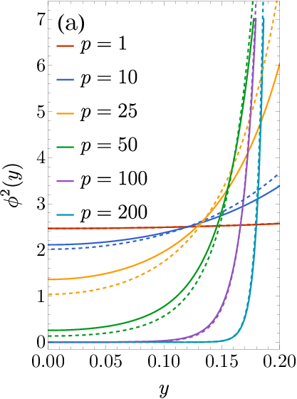
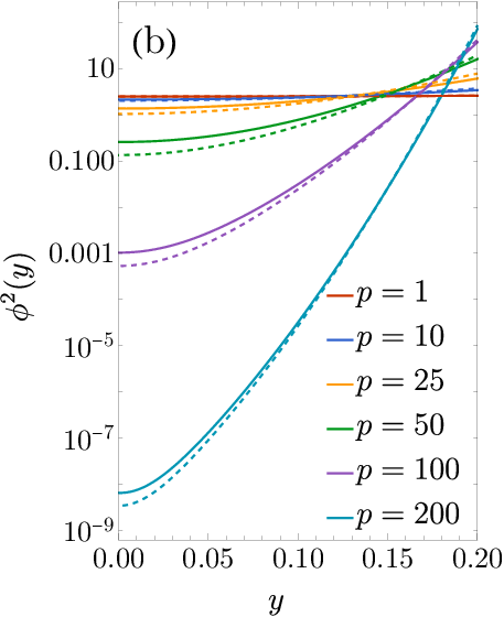
Figure 4 shows a comparison between the exact (numerical) transverse density profile coming from Eq. (3) and the EPA analytical profile, Eq. (22a), for $\epsilon=0.4$ and some representative values of $p$. It should be noted that here the normalization constant $\mathcal{N}$ is not given by Eq. (23) but is instead obtained by requiring fulfillment of Eq. (4). Although this normalization constant is not needed in Eq. (31), it is used in Fig. 4.

We observe that, even though the EPA was based on the exact high-pressure limit behavior, a good agreement with the numerical solution is reached for all pressure ranges, including the low-pressure regime, where the solution $\phi\approx\text{const}$ is recovered. In fact, we find that the worst agreement is centered around the medium pressure regime. Similar results can also be found for other values of the width parameter $\epsilon$.

Figure 5 compares the exact and approximate values of $B_{3}^{\prime}/\epsilon^{4}$ and $B_{4}^{\prime}/\epsilon^{6}$. As can be observed, the EPA predictions are more accurate than the UPA ones. On the other hand, since $B_{3}^{\prime}$ and $B_{4}^{\prime}$ are rather small, the conventional virial coefficients $B_{3}$ and $B_{4}$ are dominated by $B_{2}^{2}$ and $B_{2}^{3}$, respectively [see Eq. (11)]. Thus, the impact on $B_{3}$ and $B_{4}$ of the deviations observed in Fig. 5 is very small. At the maximum excess width, $\epsilon_{\max}=\sqrt{3}/2\simeq 0.866$, we have observed that the relative deviations in $B_{3}$ are approximately $0.3\%$ (UPA) and $-0.03\%$ (EPA), while, in the case of $B_{4}$, they are approximately $-0.5\%$ (UPA) and $0.04\%$ (EPA).

The equation of state involves performing the integrals in Eq. (8) once the density profiles (either exact or approximate) are known.

Figure 6 depicts the comparison between the two proposed approximations and the results coming from both the numerical evaluation of the exact solution for the Q1D fluid and independently calculated MC simulations for the original confined 2D system.Mon 2020 It shows a good agreement with the UPA under low-pressure and/or narrow-pore conditions, and a very good agreement with the EPA for practically all ranges of pressure and pore sizes. In the case of the EPA, the results disagree visibly from the exact solution only within a small region of medium pressures for large values of the pore size. It is interesting to note that the compressibility factor, especially with an excess pore width $\epsilon=0.80$, presents two inflection points, a feature captured even by the UPA. Although the system lacks a true phase transition, those two inflection points can be seen as precursors of the phase transition in genuine 2D systems.Bernard and Krauth 2011; Godfrey and Moore 2014

Even though the transfer-matrix solution and our approximations were developed only for nearest-neighbor interactions (single-file condition), which precludes an excess width of the channel larger than $\epsilon_{\mathrm{max}}=\sqrt{3}/2$, it is also of interest to study how well the theoretical treatments behave when this limit is exceeded.Kofke and Post 1993 In that case, the function $a(s)$ defined by Eq. (1) must be supplemented as $a(s)=0$ if $s>1$.Kofke and Post 1993 A comparison with MC simulation dataKofke and Post 1993 for $\epsilon=1$ and $1.118$ is shown in Fig. 7. We observe that, as density or pressure increases, none of the three methods is accurate. Paradoxically, however, the UPA performs a reasonable job and is perhaps the most reliable approximation in the case $\epsilon=1.118$.

In the transfer-matrix formalism, as well as in our approximations, the final computation of $Z$ must be performed numerically (see Appendix D). It is then worth studying the different execution times (the so-called wall timesWikipedia 2022a) in order to assess the cost of using the exact solution against any of the two approximations proposed in this paper.

Figure 8 shows the UPA-to-exact and EPA-to-exact wall time ratios. We clearly see that both approximations are much faster than the exact evaluation for all ranges of pressure and pore sizes, and that this wall time advantage increases with the increasing pressure and pore width. For the EPA, this is especially relevant in the case of large pore sizes and high pressures, where the performance of the EPA is excellent (see Fig. 6). In the case of the UPA, the gain in wall time is still very remarkable even for small pore sizes and small or moderate pressures, where both the exact solution and the UPA practically yield the same results (see again Fig. 6).

The authors have no conflicts to disclose.

Ana M. Montero: Formal analysis (equal); Investigation (equal); Methodology (equal); Software (lead); Writing – original draft (lead). Andrés Santos: Conceptualization (lead); Formal analysis (equal); Funding acquisition (lead); Investigation (equal); Methodology (equal); Supervision (lead); Writing – original draft (supporting); Writing – review & editing (lead).

References

- Kyakuno et al. (2011) H. Kyakuno, K. Matsuda, H. Yahiro, Y. Inami, T. Fukuoka, Y. Miyata, K. Yanagi, Y. Maniwa, H. Kataura, T. Saito, M. Yumura, and S. Iijima, “Confined water inside single-walled carbon nanotubes: Global phase diagram and effect of finite length,” J. Chem. Phys. 134, 244501 (2011).
- Majumder, Chopra, and Hinds (2011) M. Majumder, N. Chopra, and B. J. Hinds, “Mass transport through carbon nanotube membranes in three different regimes: Ionic diffusion and gas and liquid flow,” ACS Nano 5, 3867–3877 (2011).
- Boda et al. (2008) D. Boda, W. Nonner, D. Henderson, B. Eisenberg, and D. Gillespie, “Volume exclusion in calcium selective channels,” Biophys. J. 94, 3486–3496 (2008).
- Poncet et al. (2021) A. Poncet, A. Grabsch, P. Illien, and O. Bénichou, “Generalized correlation profiles in single-file systems,” Phys. Rev. Lett. 127, 220601 (2021).
- Horner and Pohl (2018) A. Horner and P. Pohl, “Single-file transport of water through membrane channels,” Faraday Discuss. 209, 9–33 (2018).
- Barker (1962) J. Barker, “Statistical mechanics of almost one-dimensional systems,” Aust. J. Phys., 15, 127–134 (1962).
- Barker (1964) J. Barker, “Statistical mechanics of almost one-dimensional systems. II,” Aust. J. Phys., 17, 259–268 (1964).
- Wojciechowski, Pierański, and Małecki (1982) K. W. Wojciechowski, P. Pierański, and J. Małecki, “A hard-disk system in a narrow box. I. Thermodynamic properties,” J. Chem. Phys. 76, 6170–6175 (1982).
- Post and Kofke (1992) A. J. Post and D. A. Kofke, “Fluids confined to narrow pores: A low-dimensional approach,” Phys. Rev. A 45, 939–952 (1992).
- Kofke and Post (1993) D. A. Kofke and A. J. Post, “Hard particles in narrow pores. Transfer-matrix solution and the periodic narrow box,” J. Chem. Phys. 98, 4853–4861 (1993).
- Percus (2002) J. K. Percus, “Density functional theory of single-file classical fluids,” Mol. Phys. 100, 2417–2422 (2002).
- Kamenetskiy, Mon, and Percus (2004) I. E. Kamenetskiy, K. K. Mon, and J. K. Percus, “Equation of state for hard-sphere fluid in restricted geometry,” J. Chem. Phys. 121, 7355–7361 (2004).
- Forster, Mukamel, and Posch (2004) C. Forster, D. Mukamel, and H. A. Posch, “Hard disks in narrow channels,” Phys. Rev. E 69, 066124 (2004).
- (14) S. Varga, G. Balló, and P. Gurin, “Structural properties of hard disks in a narrow tube,” J. Stat. Mech. 2011, P11006.
- Gurin and Varga (2013) P. Gurin and S. Varga, “Pair correlation functions of two- and three-dimensional hard-core fluids confined into narrow pores: Exact results from transfer-matrix method,” J. Chem. Phys. 139, 244708 (2013).
- Godfrey and Moore (2014) M. J. Godfrey and M. A. Moore, “Static and dynamical properties of a hard-disk fluid confined to a narrow channel,” Phys. Rev. E 89, 032111 (2014).
- Godfrey and Moore (2015) M. J. Godfrey and M. A. Moore, “Understanding the ideal glass transition: Lessons from an equilibrium study of hard disks in a channel,” Phys. Rev. E 91, 022120 (2015).
- Hu, Fu, and Charbonneau (2018) Y. Hu, L. Fu, and P. Charbonneau, “Correlation lengths in quasi-one-dimensional systems via transfer matrices,” Mol. Phys. 116, 3345–3354 (2018).
- Mon (2014) K. K. Mon, “Third and fourth virial coefficients for hard disks in narrow channels,” J. Chem. Phys. 140, 244504 (2014).
- Mon (2015) K. K. Mon, “Erratum: ‘Third and fourth virial coefficients for hard disks in narrow channels’ [J. Chem. Phys. 140, 244504 (2014)],” J. Chem. Phys. 142, 019901 (2015).
- Mon (2020) K. K. Mon, “Analytical evaluation of third and fourth virial coefficients for hard disk fluids in narrow channels and equation of state,” Physica A 556, 124833 (2020).
- Huerta et al. (2020) A. Huerta, T. Bryk, V. M. Pergamenshchik, and A. Trokhymchuk, “Kosterlitz-Thouless-type caging-uncaging transition in a quasi-one-dimensional hard disk system,” Phys. Rev. Res. 2, 033351 (2020).
- Pergamenshchik (2020) V. M. Pergamenshchik, “Analytical canonical partition function of a quasi-one-dimensional system of hard disks,” J. Chem. Phys. 153, 144111 (2020).
- Pergamenshchik, Bryk, and Trokhymchuk (2022) V. M. Pergamenshchik, T. M. Bryk, and A. Trokhymchuk, “Correlation functions and ordering in a quasi-one dimensional system of hard disks from the exact canonical partition function,” arXiv:2206.05980 (2022), 10.48550/arXiv.2206.05980.
- Jung and Franosch (2022) G. Jung and T. Franosch, “Structural properties of liquids in extreme confinement,” Phys. Rev. E 106, 014614 (2022).
- Krapivsky, Mallick, and Sadhu (2014) P. L. Krapivsky, K. Mallick, and T. Sadhu, “Large deviations in single-file diffusion,” Phys. Rev. Lett. 113, 078101 (2014).
- Robinson, Godfrey, and Moore (2016) J. F. Robinson, M. J. Godfrey, and M. A. Moore, “Glasslike behavior of a hard-disk fluid confined to a narrow channel,” Phys. Rev. E 93, 032101 (2016).
- Taloni et al. (2017) A. Taloni, O. Flomenbom, R. Castañeda-Priego, and F. Marchesoni, “Single file dynamics in soft materials,” Soft Matter 13, 1096–1106 (2017).
- Wittmann, Löwen, and Brader (2021) R. Wittmann, H. Löwen, and J. M. Brader, “Order-preserving dynamics in one dimension – single-file diffusion and caging from the perspective of dynamical density functional theory,” Mol. Phys. 119, e1867250 (2021).
- Lapolla and Godec (2020) A. Lapolla and A. Godec, “Single-file diffusion in a bi-stable potential: Signatures of memory in the barrier-crossing of a tagged-particle,” J. Chem. Phys. 153, 194104 (2020).
- Huerta et al. (2021) A. Huerta, T. Bryk, V. M. Pergamenshchik, and A. Trokhymchuk, “Collective dynamics in quasi-one-dimensional hard disk system,” Front. Phys. 9, 636052 (2021).
- Rana and Sadhu (2023) J. Rana and T. Sadhu, “Large deviations of a tracer position in the dense and the dilute limits of a single-file diffusion,” Phys. Rev. E 107, L012101 (2023).
- Mayo et al. (2022) M. Mayo, J. J. Brey, M. I. García de Soria, and P. Maynar, “Kinetic theory of a confined quasi-one-dimensional gas of hard disks,” Physica A 597, 127237 (2022).
- (34) P. Rizkallah, A. Grabsch, P. Illien, and O. Bénichou, “Duality relations in single-file diffusion,” J. Stat. Mech. 2023, 013202.
- Maynar, García de Soria, and Brey (2022) P. Maynar, M. I. García de Soria, and J. J. Brey, “Dynamics of an inelastic tagged particle under strong confinement,” Phys. Fluids 34, 123321 (2022).
- Zhang, Godfrey, and Moore (2020) Y. Zhang, M. J. Godfrey, and M. A. Moore, “Marginally jammed states of hard disks in a one-dimensional channel,” Phys. Rev. E 102, 042614 (2020).
- Ikeda (2020) H. Ikeda, “Jamming below upper critical dimension,” Phys. Rev. Lett. 125, 038001 (2020).
- Liu and Müller (2020) D. Liu and G. Müller, “Jammed disks of two sizes in a narrow channel,” in Traffic and Granular Flow 2019, edited by I. Zuriguel, A. Garcimartin, and R. Cruz (Springer International Publishing, Cham, 2020) pp. 389–395.
- Liu and Müller (2022) D. Liu and G. Müller, “Jammed disks of two sizes and weights in a channel: Alternating sequences,” Phys. Rev. E 105, 024904 (2022).
- Tonks (1936) L. Tonks, “The complete equation of state of one, two and three-dimensional gases of hard elastic spheres,” Phys. Rev. 50, 955–963 (1936).
- Hansen and McDonald (2013) J.-P. Hansen and I. R. McDonald, Theory of Simple Liquids, 4th ed. (Academic Press, London, 2013).
- Santos (2016) A. Santos, A Concise Course on the Theory of Classical Liquids. Basics and Selected Topics, Lecture Notes in Physics, Vol. 923 (Springer, New York, 2016).
- Mon (2018) K. K. Mon, “Virial series expansion and Monte Carlo studies of equation of state for hard spheres in narrow cylindrical pores,” Phys. Rev. E 97, 052114 (2018).
- Caracciolo, Mognetti, and Pelissetto (2006) S. Caracciolo, B. M. Mognetti, and A. Pelissetto, “Virial coefficients and osmotic pressure in polymer solutions in good-solvent conditions,” J. Chem Phys. 125, 094903 (2006).
- Maestre et al. (2011) M. A. G. Maestre, A. Santos, M. Robles, and M. López de Haro, “On the relation between virial coefficients and the close-packing of hard disks and hard spheres,” J. Chem. Phys. 134, 084502 (2011).
- Bernard and Krauth (2011) E. P. Bernard and W. Krauth, “Two-step melting in two dimensions: First-order liquid-hexatic transition,” Phys. Rev. Lett. 107, 155704 (2011).
- Wikipedia (2022a) Wikipedia, “Elapsed real time,” https://en.wikipedia.org/wiki/Elapsed_real_time (2022a).
- Montero (2023) A. M. Montero, “SingleFileHardDisks,” https://github.com/amonterouex/SingleFileHardDisks (2023).
- Wikipedia (2022b) Wikipedia, “Gauss–Kronrod quadrature formula,” https://en.wikipedia.org/wiki/Gauss-Kronrod_quadrature_formula (2022b).