Convergence Analysis for Training Stochastic Neural Networks via Stochastic Gradient Descent
Abstract
In this paper, we carry out numerical analysis to prove convergence of a novel sample-wise back-propagation method for training a class of stochastic neural networks (SNNs). The structure of the SNN is formulated as discretization of a stochastic differential equation (SDE). A stochastic optimal control framework is introduced to model the training procedure, and a sample-wise approximation scheme for the adjoint backward SDE is applied to improve the efficiency of the stochastic optimal control solver, which is equivalent to the back-propagation for training the SNN. The convergence analysis is derived with and without convexity assumption for optimization of the SNN parameters. Especially, our analysis indicates that the number of SNN training steps should be proportional to the square of the number of layers in the convex optimization case. Numerical experiments are carried out to validate the analysis results, and the performance of the sample-wise back-propagation method for training SNNs is examined by benchmark machine learning examples.
Keywords. Probabilistic learning, stochastic neural networks, convergence analysis, backward stochastic differential equations, stochastic gradient descent
1 Introduction
Deep neural network (DNN) based machine learning techniques are positioned to fundamentally change many sectors of society by offering decision making capabilities, which match and often exceed that of human experts [20, 39, 34, 35, 36, 33, 1]. Despite of dramatic success that DNNs achieved, a closer examination reveals inherent challenges of applying such approaches broadly to science and engineering. A major challenge is that DNN models are sensitive to noises in data. A recent study [10] shows that effectiveness of different DNN models are affected by inaccurate data in the datasets, and science and engineering solutions typically need to be able to quantify the uncertainty of DNN outputs and to provide effective operating ranges and risks.
One successful effort to address the challenge of uncertainty quantification for DNN is probabilistic learning, which aims to incorporate randomness to DNN models and produce random output. Then, one can use the statistical behaviors of DNN’s random output to study the uncertainty of data. The state-of-the-art probabilistic learning approach is the Bayesian neural network (BNN) [16, 17, 24, 30, 31, 38, 40, 41], which treats parameters in a DNN as random variables and approximates their distributions through Bayesian inference. Instead of searching for the optimal parameters by deterministic optimization, the BNN utilizes Bayesian optimization to derive parameter distributions. As a result, the estimated random parameters generate random output, which characterizes the target model’s uncertainty. Although the BNN approach provides a principled conceptual framework to quantify the uncertainty in probabilistic machine learning, carrying out Bayesian optimization to estimate a massive number of parameters in the BNN often renders the exact inference of parameter posteriors intractable. Moreover, the large size of the parameter set leads to uninterpretable parameter priors. Some of the existing Non-Bayesian methods, such as [15, 25], are simple to implement but either ad hoc or computationally prohibitive.
In this work, we consider a type of stochastic neural networks that models uncertainty in some of the well known DNN structures (e.g., residual neural networks, convolutional neural networks) through discretized stochastic (ordinary) differential equations (SDEs). Recently, an ordinary differential equation (ODE) interpretation for DNNs (named Neural-ODE) has been introduced and studied [11, 12, 13, 18, 19]. The central idea of the Neural-ODE is to formulate the evolution of potentially huge hidden layers in the DNN as a discretized ODE system. To characterize the randomness caused by the uncertainty of models and noises of data, we add an additive Brownian motion noise to the ODE to count for the model uncertainty of the DNN. This changes the ODE to an SDE, and the deterministic DNN becomes a stochastic neural network (SNN) [23, 28, 37]. In the SNN model, the drift parameters serve as the prediction of the network, and the stochastic diffusion governs the randomness of network output, which serves to quantify the uncertainty of deep learning. In comparison with the BNN, which needs to calibrate tremendous amount of random parameters through Bayesian inference, the SNN only uses one noise term (i.e., the diffusion term) to control the amount of uncertainty at each layer. Apparently, the computational cost for evaluating the diffusion coefficient is much lower than high-dimensional Bayesian inference for a large number of unknown random parameters. On the other hand, for an SNN with multiple hidden layers, by stacking (controlled) diffusion terms together through the multi-layer structure, we would still be able to characterize sufficient probabilistic behavior of the neural network.
The bottleneck of the SNN is constructing an efficient numerical solver for the back-propagation. This process propagates the total loss back into the neural network and updates the parameters accordingly to minimize the loss. It is the essence of neural network training. For Neural-ODE, back-propagation is equivalent to solving the adjoint of the ODE, which is a backward ODE. Since its structure is no different from that of a forward ODE, back-propagation can be achieved by means of a deterministic adjoint ODE solver [11]. For SNNs, the back-propagation is equivalent to solving the adjoint of the SDE, which is a backward SDE. Because of the martingale nature of the backward SDE [14], one must create a separate backward SDE solver which is completely different from and far more computationally intensive than forward SDE solvers. Thus the back-propagation by completely solving the backward SDE has been deemed unfeasible [37]. Several alternatives have been proposed [23, 28, 37]. But they either fail to consider the Ito’s nature of stochastic differentiation or lack scalability. Thus these training frameworks have been deemed inefficient [27]. In a recent study [2], we formulated the training procedure for SNN as a stochastic optimal control problem, and introduced a sample-wise scheme for solving the backward SDE corresponding to the forward propagation of the SNN and constructed a novel back-propagation solver. A central idea of our method is to treat the random samples of the backward SDE as “pseudo data”, and only solve the backward SDE partially on randomly selected pseudo data. In this way, only a tiny fraction of the computing cost of solving the entire backward SDE is required to complete one training iteration. Therefore, our novel sample-wise back-propagation method for SNNs will be a feasible tool for the uncertainty quantification of deep learning. Although the sample-wise back-propagation procedure does not produce accurate numerical solutions for backward SDEs, we want to point out that the solutions of the adjoint equation are only used to construct the gradient process for gradient descent optimization, and obtaining complete numerical solutions for backward SDEs is not necessary in the back-propagation procedure.
The contribution of this work has a theoretical aspect and a numerical implementation aspect. Our theoretical contribution will focus on deriving convergence analysis for the sample-wise back-propagation algorithm. Different from classic convergence results for stochastic gradient descent (SGD) based optimization, the main challenge in the convergence analysis for our sample-wise back-propagation solver is that the gradient process is formulated by (discrete) approximated solutions for the adjoint backward SDE, and classic numerical methods for solving backward SDEs require obtaining complete numerical approximations for the solutions in the entire state space [43]. However, a sample-wise approximation (or an approximation on mini-batch) for the solution does not carry enough information to deduce convergence of the numerical solver with standard techniques for backward SDEs. Our strategy to address this issue is to introduce an augmented -algebra that contains the uncertainty information in both the SNN model and the training data. After proving some basic properties for the sample-wise approximators, we can derive that the stochastic approximation for the gradient conditioning on the augmented -algebra is an unbiased estimator. This result would help us obtain our main convergence theorems without usage of general convergence of numerical solvers for backward SDEs. In this paper, we first assume that the optimization problem for searching the optimal SNN parameters (or equivalently the optimal control) is convex, which is a classic assumption in most existing numerical analysis results for stochastic optimal control problems. Our analysis under the convexity assumption shows that the sample-wise back-propagation algorithm will result in two (mean square) error terms: The first error term gives half-order convergence with respect to the depth of neural networks; the second error term is a quotient of the depth of SNN and the number of training steps. While the half-order convergence with respect to the depth indicates convergence of the discrete SNN model in approximating the continuous SDE formulation of probabilistic learning, the quotient error term can provide inherent relation between the depth of a neural network and the number of iterations needed in the training procedure. Although several analysis outcomes have been derived to study convergence of training with respect to SGD iterations, very limited research is conducted to explore the inherent connection between the depth of a neural network and the number of training iterations that is needed. Moreover, since the convexity assumption may not hold in many practical machine learning applications, we will also derive a convergence theorem without assuming the optimization problem is convex. Specifically, we will show that for an SNN with a fixed depth, our proposed sample-wise back-propagation algorithm will converge with respect to training steps.
In addition to the effort on deriving theoretical analysis results, in this paper we shall carry out various numerical experiments to examine the performance of our sample-wise back-propagation method, and we will adopt well established DNN structures to the SNN model when solving practical machine learning problems. Specifically, besides demonstration examples of synthetic mathematical problems, which are designed to showcase the baseline performance and convergence behavior of our algorithm, we will also solve the benchmark classification problem with MNIST handwritten dataset and Fashion-MNIST dataset. To enhance the learning capability of SNNs to accomplish the classification task, convolution blocks are incorporated into the SNN model in the numerical implementation. Other DNN structures can be adopted in a similar way to solve machine learning problems in different scenarios. Through our numerical experiments, we will validate the theoretical results that we derived in this paper, and we will present the stability/robustness advantage of SNN (as a probabilistic learning method) compared with the conventional deterministic convolution neural network.
The rest of this paper is organized as follows: In Section 2, we formulate the training procedure for SNNs as a stochastic optimal control problem and briefly introduce our sample-wise back-propagation method. The main convergence theorems and their proofs will be provided in Section 3. In Section 4, we will validate our analysis results and examine the performance of SNNs through several numerical experiments.
2 A sample-wise back-propagation method for stochastic neural networks
In this section, we introduce our sample-wise back-propagation method for training stochastic neural networks. We first formulate the training procedure for the continuous formulation of a stochastic neural network as a stochastic optimal control problem. Then we solve this stochastic optimal control problem via a stochastic gradient descent algorithm.
2.1 Stochastic optimal control formulation for SNN
We consider the following dynamical system for a stochastic version of deep neural network (DNN):
| (2.1) |
where is a vector that contains neurons at the -th layer in a DNN, is an activation function, denotes the set of DNN parameters at the -th layer, is a positive constant that stabilizes the DNN, is a standard -dimensional Gaussian random variable that brings uncertainty to the neural network, and is a coefficient function that determines the size of uncertainty in the DNN. Since the uncertainty of the DNN is incorporated by the Gaussian random variables, we assume that parameters are deterministic. The initial state of the dynamical system (2.1) represents the input layer, and is the output layer, which will be compared with data. We call the noise perturbed DNN model (2.1) a stochastic neural network (SNN) in this paper.
If we choose a positive constant (as a terminal time) and let or with , the dynamics of SNN (2.1) becomes the stochastic differential equation (SDE) which, in the integral form, is given by
| (2.2) |
where is a standard Brownian motion corresponding to the i.i.d. Gaussian random variable sequence in (2.1), is an Itô integral. is now corresponding to the output layer. Let be the random variable that generates the training data to be compared with and define a loss function corresponding to a loss error norm . The goal of the training procedure for deep learning is to determine the optimal parameter to minimize the loss function.
In this paper, we shall treat the training procedure for deep learning as a stochastic optimal control problem and the parameter in (2.2) as a control process. To this end, we define the cost functional as
| (2.3) |
where the integral represents the running cost in a control problem. In this way, the loss function becomes the terminal cost in the stochastic optimal control problem. Note that the stochastic process is the “state process” for the stochastic optimal control problem which depends on the control . The goal of deep learning is to solve the stochastic optimal control problem, i.e., find the optimal control such that
| (2.4) |
where is a -dimensional admissible control set.
In order to determine the optimal control, one can derive the following gradient process [29, 42]:
| (2.5) |
where , and are partial derivatives with respect to the control . In this paper, we use the notation to denote the gradient of the cost with respect to the control process , and the control at time , i.e., , in indicates that we are considering the gradient process at time . Here the stochastic processes and in (2.5) are the adapted solutions of the following backward SDE:
| (2.6) |
where , are partial derivatives with respect to the state , is the adjoint process of the state SDE , and is the martingale representation of with respect to . An important property of solutions of the backward SDE is that values of and depend on , and , where .
Then, one can carry out gradient descent optimization to determine the optimal control by using the gradient introduced in (2.5) as follows:
| (2.7) |
where is an initial guess for the optimal control, is the step-size of gradient descent in the -th iteration step, and is a projection operator onto the admissible control set .
Numerical implementation of the gradient descent optimization scheme (2.7) requires numerical approximations for solutions , and of the backward SDE (2.6). In the following subsection, we shall first introduce numerical schemes to approximate and , and then utilize stochastic approximation to efficiently carry out a stochastic gradient descent procedure to determine the optimal control.
2.2 Numerical schemes for backward SDEs and stochastic gradient descent optimization
We solve the backward SDE (2.6) over a uniform temporal partition . Denote by the stepsize of the partition. On each subinterval , , the backward SDE satisfies
| (2.8) |
We introduce the following Euler-Maruyama scheme to approximate the forward SDE (2.2) on interval :
| (2.9) |
where , and denotes the approximation errors of deterministic and stochastic integrals.
To approximate solution , we take conditional expectation on both sides of (2.8) and approximate the deterministic integral by using the right-point formula to get
| (2.10) |
where is the approximation error, and we denote since is measurable. Note that the stochastic integral is eliminated under expectation.
To get an approximation for , we multiply on both sides of (2.8) and then take conditional expectation to get
We use the left-point formula to approximate both the deterministic and the stochastic integral in the above equation and obtain
| (2.11) |
where is the approximation error.
By dropping the approximation error terms , and in (2.9), (2.10) and (2.11), respectively, we get the following numerical schemes to solve the backward SDE (2.6) (see [43, 44, 3, 4, 5, 6, 7, 8] for more details):
| (2.12) |
| (2.13) | ||||
where , and are numerical approximations for , and , respectively. The reason that we can remove the conditional expectation for and on the left hand side of Eq. (2.13) is due to that fact that and are adapted to . Then, we replace , and in (2.5) with our numerical solutions and obtain a piece-wise approximation for over the interval as follows:
| (2.14) |
To calculate the gradient through scheme (2.14), we need to evaluate the expectation (with respect to the state process ). In addition, the approximate solutions and are under the conditional expectation . The conventional approach for simulating expectations is the Monte Carlo method. However, when using stochastic optimal control to formulate the training procedure of the SNN, the dimension of the state is equivalent to the number of neurons. Hence it requires very large number of Monte Carlo samples to approximate expectations, and the computational cost for calculating the gradient in each gradient descent iteration step is very high. Moreover, note that and depend on , which is typically represented by a set of pre-chosen points in the state space. Therefore, interpolation methods are needed to calculate and at random state points in order to implement the Monte Carlo simulation. This is a very challenging task due to “curse of dimensionality”.
To address the above challenges, we apply the stochastic approximation method to approximate expectations in the approximation scheme (2.14) for the gradient . Specifically, at the -th iteration step with an estimated optimal control , we simulate the state process by choosing a sample and get
| (2.15) |
Instead of using the average of a large number of Monte Carlo samples, we approximate the expectations in schemes (2.13) with the single-realization of the simulate sample path and obtain the following sample-wise solution for and :
| (2.16) |
where and are approximations for and , respectively. Although schemes (2.16) do not produce numerical solutions for and in the entire state space, the solutions and of the backward SDE (2.6) only appear in the gradient process, and complete numerical solutions for and in the entire state space are not necessary in the gradient descent optimization procedure for the optimal control. In this way, the justification for application of stochastic approximation in stochastic gradient descent can be used to explain the design of the sample-wise approximation scheme (2.16). Therefore, we approximate the gradient by the following scheme
| (2.17) |
and we carry out stochastic gradient descent (SGD) optimization to search for the optimal control as follows:
| (2.18) |
where with a piece-wise constant approximation set for the control process.
The above schemes (2.15) - (2.18) provide an SGD algorithm for solving the stochastic optimal control problem, and it also constitutes a sample-wise back-propagation framework for training the SNN. It’s worthy to mention that in machine learning practice, the above sample-wise back-propagation scheme is often implemented by using a mini-batch of samples instead of a single-realization of sample to represent the state variable. For convenience of presentation, we shall use the single sample representation in the rest of this paper. The numerical implementation and analysis for the mini-batch case can be derived following a similar strategy.
3 Convergence Analysis
In this section, we conduct the convergence analysis for the SGD algorithm (2.15) - (2.18), and we have the following standard assumptions for backward SDEs and the stochastic optimal control problem [44, 42]:
Assumption 3.1.
- (a)
Both and belong to .
- (b)
, , , , , , are uniformly bounded and Lipschitz in and .
- (c)
satisfies the uniform elliptic condition.
- (d)
The initial condition .
- (e)
The loss function is and positive, and has at most linear growth at infinity.
- (f)
.
We define the standard inner product of by and the standard norm by . Without confusion, we use the same notation to denote the inner product of two piece-wise constant representations , of , : . Also, we use to denote the Euclidean norm or Frobenius norm.
Our analysis in this paper will focus on the convergence with respect to the temporal partition . Convergence regarding the number of neurons, i.e., the dimension of the state in SDE (2.2), may bring out more complicated discussions on spatial dimension approximation and representability of neural networks, which is out of scope of this paper. Specifically, we will derive convergence theorems under two scenarios. First, we assume that the cost functional for the optimal control is convex and prove a half-order convergence rate for our algorithm. In the second situation, we consider the case without convexity assumption and provide a convergence result for our sample-wise back-propagation method.
3.1 Preliminaries
The foundation of the convergence analysis is based on the fact that the sample-wise solutions and introduced in (2.16) are equivalent to the classic numerical solutions and introduced in (2.13) under conditional expectation . Specifically, we have the following proposition.
Proposition 3.2.
For given estimated control , let and be the numerical solutions defined in (2.13) driven by . Then following identities hold:
| (3.1) |
and therefore we have and .
Proof.
Note that the random variable in scheme (2.15) has the same distribution of appeared in (2.12). Hence, the random variable is equivalent to under expectation. More generally, for any function of the random sample path , we have .
To obtain the desired results in the proposition, we first consider the case (i.e. take one step back from the terminal time), and we have
Following the same argument, we also have
Since and , where is the approximated solution introduced in (2.12) with the given control , the above equation becomes
| (3.2) |
Then, by repeatedly applying the equality (3.2) and the tower property, we obtain the desired result (3.1). ∎
To proceed, we let be an augmented -algebra generated by the Gaussian random variables , which we use to generate state sample path in the sample-wise scheme (2.15), and the data sample , which is generated by the training data variable . Based on the above proposition, we see that the stochastic approximation that we introduced in (2.17) is an unbiased estimator for the gradient given , i.e. . From scheme (2.18), we observe that the estimated optimal control is measurable, and we denote in the rest of this paper for convenience of presentation. Therefore, similar to the argument in the proof for Proposition 3.2, we have
In the following lemma, we provide the boundedness property of the sample-wise solution and the linear growth property for with for any approximate control .
Lemma 3.3.
Under Assumptions (a)-(e), for any , we have
for some positive constant .
Proof.
We square both sides of the scheme for defined in (2.16) and then take expectation to get
where we have used the Young’s inequality. Then, by the discrete Gronwall inequality, we have
Due to the Assumption 3.1 (e) for the loss function , we have that as desired.
Next, we square both sides of the scheme for and take expectation. Based the boundedness for , we have that
which is the desired boundedness for . ∎
In addition, we have the following classic boundedness property for solutions of backward SDEs (see Theorem 4.2.1 in [43]):
| (3.3) |
which will provide the following boundedness result
| (3.4) |
for the analytic solutions and driven by a control , where the constant is independent of . Following the above estimates, one can also show that under Assumption 3.1 (a)-(e).
Note that the boundedness of the sample-wise solution in the estimate in Lemma 3.3 is not as strong as the true solution due to the loss of regularity caused by the sample-wise representation of expectation introduced in (2.16).
The next proposition is about the convergence of the numerical solutions to backward SDEs introduced in (2.13) also holds:
Proposition 3.4.
Under Assumption 3.1, for small enough step-size , there exists independent of such that
| (3.5) |
Proof.
The inequality (3.5) is a standard extension of the regularity property, and the proof of the theorem can be derived following the proof for Theorem 5.3.3 in [43]. The fact that does not depend on is due to the uniform boundedness and the Lipschitz assumptions of , and .
∎
The boundedness property of solutions of backward SDEs gives us the boundedness of . Also, the convergence result (3.5) gives the boundedness of , which makes bounded, i.e.
| (3.6) |
As a consequence of the above discussions, we have the following lemma.
Lemma 3.5.
Under Assumption 3.1, for any piece-wise constant estimated control , the following estimation holds
| (3.7) |
Proof.
Due to Lemma 3.3 and the boundedness assumptions for , and , we have that
| (3.8) |
Then, we can obtain
where is a generic constant that is independent from . Hence we can get the desired result of the lemma from the above analysis. ∎
3.2 Convergence analysis: strongly convex cost functional
Here, we assume that the cost functional defined in (2.3) is strongly convex in the following sense: there exists some constant such that for any control terms ,
| (3.9) |
By the Assumption 3.1, we have the following smoothness result for with a positive constant :
or equivalently,
| (3.10) |
Before stating the main convergence theorem, we need an estimate about the error between the true gradient and the piece-wisely approximated gradient .
Lemma 3.6.
Assume that Assumption 3.1 holds and , . Then there exists a constant such that
| (3.11) |
Proof.
Denote
We have that
∎
Let be the optimal control for the stochastic optimal control problem (2.4) found in the subset of the admissible control set . Then, we have the following estimate.
Lemma 3.7.
The following inequality holds:
| (3.12) |
Proof.
Let be the projection of onto , i.e. . Due to the boundedness of , we have
Since the solutions of the backward SDEs are bounded, is also bounded. Thus
Hence
By the strong convex assumption, we have
Since , the above inequality leads to
| (3.13) |
The desired result of the lemma is obtained by the above estimate and the convexity assumption (3.10). ∎
Since , as a direct consequence of (3.12), we have
| (3.14) |
Now we are ready to prove the main convergence results of our algorithm under the convexity assumption. First we estimate the error between the exact solution of the optimal control and the optimal control in the piece-wise constant subset of the admissible set .
Theorem 3.8.
Proof.
Recall that is the optimal control found in the control set . Hence
| (3.16) |
Then, we subtract (3.16) from the SGD optimization scheme (2.18) to get
By taking conditional expectation to the above equation and then applying the Young’s inequality, we obtain
| (3.17) | ||||
From the convexity assumption (3.9) and Lemma 3.6, we can deduce by using the Young’s inequality with and the fact that is measurable to get
| (3.18) | ||||
Moreover, from Lemma 3.5, Lemma 3.6 and the convexity assumption (3.10), we have
| (3.19) | ||||
where we use to denote a generic constant independent of , and controls.
Let . We can find and such that
and we have that when is large enough, for . By picking in (3.20), we have
Next, we take expectation to both sides of the above estimate and apply it recursively from to to get
Since and , the above estimate gives us
∎
Note that the estimate (3.15) provides the convergence between the estimated control and the optimal control found in the subspace . The next theorem, which is the main result of this section, gives the convergence between and the exact optimal control .
Theorem 3.9.
Assume that all the assumptions hold in Theorem 3.8 and assume the optimal control is bounded. Then, for large enough , we have the following convergence result:
| (3.21) |
3.3 Convergence analysis for the non-convex optimization case
Now, we study the convergence of our algorithm without the convexity assumption. In this work, we introduce the running cost in the stochastic optimal control problem to the loss in machine learning, and the running cost term performs as a regularizer to stabilize the SNN in our analysis.
In addition to the boundedness assumptions in Assumption 3.1, we assume that the running cost only depends on control , and we let , which is uniformly bounded from below by , i.e.
| (3.22) |
where is a constant that satisfies Lemma 3.6. We also assume the learning rate satisfies
| (3.23) |
To proceed, we denote as the cost function corresponding to the fully calculated approximate gradient , i.e.,
Note that for any , ,
| (3.24) | ||||
Then, we can show that is bounded from below based on the boundedness assumption for the running cost , i.e.,
where is the solution of the state equation (2.2) driven by the control . We choose in the above estimate. Then, it follows from Lemma 3.6 that
which indicates that is bounded from below.
Our aim is to show that for a given depth , a.s.. To this end, we first state two propositions that can be derived following the same proofs as in Theorem 5.3.1 and Theorem 5.3.3 of [43].
Proposition 3.10.
Proposition 3.11.
Assume that Assumption 3.1 hold and let and for numerical solutions and with controls . We have the following estimate
With the above propositions, we can derive the following lemma:
Lemma 3.12.
Let . Under Assumption 3.1, there exists a positive constant such that
Proof.
Since , we can write and . Then, it follows from Proposition 3.10, Proposition 3.11 and Assumption 3.1 that
∎
We also need the following lemma.
Lemma 3.13.
Proof.
From the definition of and (3.24), we have that
Applying Lemma 3.12 to the right hand side of the above equation, we get
Hence we can rewrite the above inequality to get the following estimate
| (3.26) |
Next, we take the conditional expectation on both sides of (3.26). Similar to the argument in proving Proposition 3.2, we have
which, together with the estimate estimate (3.8), gives us
as desired. ∎
The following lemma gives the final preparation for the main theorem of this subsection.
Lemma 3.14.
Proof.
We first show that
| (3.28) |
If (3.28) is not true, there exists constants and such that for all , . As a result, we have from our assumption in (3.23) that
which contradicts the assumption (3.27) in this lemma.
On the other hand, we suppose that
| (3.29) |
Then, we can find two sequences of stopping times and defined inductively as follows: given , let
Hence, we have
Therefore, , . By (3.8) in the proof of Lemma 3.5, we have
By triangle inequality, the above estimate gives
Then, by Lemma 3.12 we obtain
| (3.30) |
By definition of stopping times and , we have
However, letting in the above inequality will result a contradiction due to (3.30).
Therefore, we have , . Together with (3.28), we obtain the desired convergence result in the lemma. ∎
Now, we introduce our main convergence theorem that shows our sample-wise back-propagation method convergences in training a -layer SNN.
Theorem 3.15.
Proof.
Let . We proceed to prove , which is the condition (3.27) in Lemma 3.14 that will give the desired result of this theorem.
Define
where is a constant that satisfies (3.25) in Lemma 3.13. Then, we apply (3.25) to get
| (3.31) |
Since is bounded from below as we discussed above, is also bounded from below. Moreover, we know from (3.31) that is a super-martingale bounded from below. Therefore, by martingale convergence theorem, we obtain
Then, we apply (3.31) to get
Then, the desired result of this theorem holds by using the conclusion in Lemma 3.14. ∎
4 Numerical experiments
In this section, we use three numerical examples to validate our theoretical results and demonstrate the performance of SNN (as a probabilistic learning method) trained by our sample-wise back-propagation algorithm. In Example 1, we solve a linear-quadratic stochastic optimal control problem, which satisfies the convexity assumption, and the analytical expression of the optimal control can be found in this example. We want to use this classic stochastic optimal control example to examine the convergence rate that we provided in Theorem 3.9. In Example 2, we present the performance of our sample-wise back-propagation method in training SNNs to learn random noise perturbed functions, and we will show the convergence trend of our algorithm in this function approximation example. We will first use a smaller scale SNN to learn a one-dimensional (1D) function, and then let SNN learn an 8D function. In the third example, we use our SNN method to solve the benchmark classification problem by using the MNIST handwritten dataset and the Fashion-MNIST dataset. We want to use this example to show that our method works well for classic machine learning tasks, and it also has the robustness advantage compared with the conventional deterministic convolution neural network. The CPU that we use to run the numerical experiments in this section is an M1 Pro Chip with 3.2GHz and 16 GB memory.
4.1 Example 1
In this example, we consider the following state process on the temporal interval :
| (4.1) |
where and are 8D state and control. The vector function is defined by
where . The cost functional is defined by
| (4.2) |
where is the Euclidean norm in , and is defined by
where . For , in the above are defined as . Since the stochastic optimal control problem (4.1)-(4.2) is a linear-quadratic problem, we can find the analytic expression for the optimal control as
In this example, we let , , and . In the first experiment, we let with iteration steps for each . In the convergence analysis (3.21) proved in Theorem 3.9, we can see that when choosing , the approximation error has half-order convergence rate. To validate this result, we solve the stochastic optimal control problem (4.1)-(4.2) repeatedly times and plot the root mean square errors (RMSEs) in Figure 1 (a).


The blue dots give the RMSEs corresponding to (presented by on the -axis), and the red straight line shows the slope of half-order convergence. From this figure, we can see that our algorithm does provide half-order convergence rate in this example when the relation is satisfied.
In Figure 1 (b), we further investigate the convergence with respect to , and we let be a fixed partition number. The blue dots show the RMSEs corresponding to different values (presented by on the -axis), and the red straight line indicates the slope of half-order convergence. From this figure, we can see that the convergence rate of our algorithm is well-aligned with the half-order slope while the number of iterations is relatively small. However, when values become larger, the accuracy of our algorithm does not always improve accordingly. This verifies the existence of the term in the analysis (3.21), which becomes the bottleneck in convergence with large iteration number . In other words, a fixed partition number limits the convergence of algorithm no matter how many iteration steps we implement in the optimization procedure.
4.2 Example 2
In this example, we use the SNN model (2.1) to learn random noise perturbed functions by using discrete function values as data and demonstrate the performance of our method in both function approximation and uncertainty quantification. We let and choose the activation function in the SNN as a bounded combination of sigmoid functions, which is defined as follows:
where is a sigmoid function, are taking values on the interval , which is a set of weights for different sigmoid functions, is the weight matrix for state of neurons, and is a bias vector.
Case 1: 1D function approximation
In this experiment, we approximate a 1D function: , , and we collect altogether noise perturbed function values, i.e. input-output pairs , as our data set.
In this experiment, we train an layer - neuron SNN and run iteration steps in the training procedure. The CPU time for this training procedure is seconds.


Then, we use the trained SNN to estimate the function. The approximated function is presented in Fig. 2 (a) by showing the mean of SNN outputs (the blue crosses) on a uniform mesh over , and the corresponding confidence band (the red dashed lines) is also presented in this figure. We can see that the SNN estimates are well-aligned with the true function mean values (the red dots), and the estimated confidence band is very close to the true function’s uncertainty band (the green lines). Note that in our analysis, we require boundedness and differentiability for the activation function in the SNN. To show that violation of boundedness and differentiability may result poor performance of SNN, we repeat the above experiment by replacing sigmoid function with a ReLu function. It is well known that ReLu is a very important activation function in deep learning, and it is a typical activation function that is not bounded and is not differentiable everywhere. In this experiment, we also train a layer - neuron SNN as we did to obtain Figure 2 (a), and the result is presented in Figure 2 (b). We can see from this figure that without boundedness and differentiability for the activation function, the SNN fails in this experiment. Since both experiments are carried out under the same environment except that the activation function is chosen as sigmoid (subplot (a)) and ReLu (subplot (b)). This verifies the necessity of boundedness and differentiability assumption in our algorithm.
Case 2: 8D function approximation
In the second experiment, we approximate the following noise perturbed 8D function:
The training data are collected on spatial mesh points in the hyper cube . Since this is a high dimensional function, we use a SNN with layer and put neurons in each layer. The number of optimization iterations that we carry out to train the SNN is , and the CPU time for this training procedure is seconds. It’s worthy to mention that each data sample contains only limited amount of information about the perturbation noise, and significant amount of computational effort in this 8-dimensional approximation example would contribute to finding the confidence band of the function, which is also the main challenge in uncertainty quantification for deep learning.


In Figure 3, we compare the real marginal surface of function (presented in mean values) with our estimated surface by using the trained SNN. In Figure 3 (a), we present the exact - marginal surface of function , and Figure 3 (b) shows the SNN learned - marginal surface; In Figure 3 (c), we present the exact - marginal surface of function , and Figure 3 (d) shows the SNN learned - marginal surface. From this figure, we can see that by training the SNN steps with our sample-wise back-propagation algorithm, it can give very good approximation for the original function.

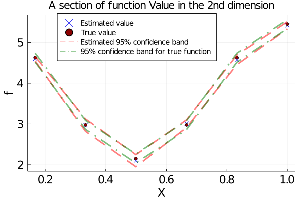
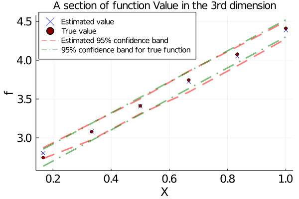
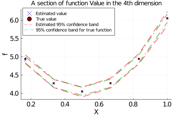
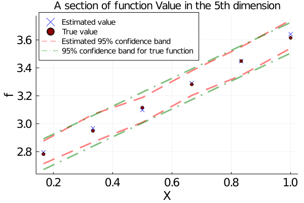
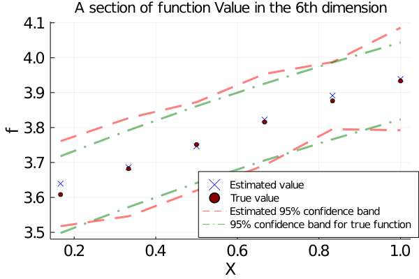
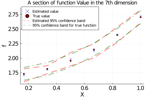
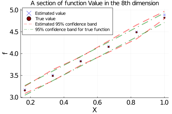
To show more details of the SNN’s performance in function approximation, we present section views of each direction in Figure 4, where the exact function mean values are plotted by red dots, the SNN estimated function mean values are plotted by blue crosses, the true uncertainty bands are presented by green dashed lines, and the SNN estimated confidence bands are presented by red dashed lines. From this figure, we can see that the trained SNN can accurately approximate the function’s mean values, as well as the uncertainty caused by the random variable .

To validate the convergence of our algorithm, we train SNNs with , and present the accuracy of function approximation and uncertainty quantification with different numbers of training steps in Figure 5 and Figure 6.

We can see from those figures that the SNN can achieve higher accuracy in estimating both function values and uncertainty bands by using more layers. For a fixed SNN depth, we can see clear convergence trend when implementing more iteration steps. However, an accuracy barrier appears in each experiment due to the fixed SNN depth, which typically result limited representation capability by using neural network models.
4.3 Example 3
In this example, we present the performance of our SNN algorithm in solving benchmark machine learning problems. Specifically, we solve the image classification problem with the MNIST handwritten digit dataset and the Fashion-MNIST dataset. In each dataset, we have 60000 training data samples and 10000 testing data samples. To enhance the learning capability of SNN to accomplish the classification task, we incorporate convolution blocks into the drift term in the SNN framework. Other DNN structures can be adopted in different machine learning scenarios. Also, instead of using a single-realization of sample to represent the state variable (as we did in the above synthetic examples), we use a mini-batch of samples to approximate expectations in our SNN algorithm. Detailed formulation of the SNN structure and our specific numerical implementation can be found on github at https://github.com/Huisun317/SNN.
In Figure 7, we present the training accuracy and testing accuracy of our SNN algorithm in solving the classification problem over the MINST handwritten dataset with different batch sizes,


and in Figure 8, we present the training accuracy and testing accuracy of our SNN algorithm in solving the classification problem over the Fashion-MINST dataset with different batch sizes.


We can see from those figures that our SNN algorithm can generate accurate classification results fairly fast (with various batch sizes) in both training and testing for bench-mark classification tasks.
To present the necessity of applying SNN as a probabilistic learning tool, we consider an adversarial game scenario, in which some “attacker” attacks the data and try to fool the neural network (pre-trained on clean dataset) while the model retrains itself along the way using the attacked dataset to play an adversarial game against the attacker. We want to use this experiment to show that our SNN algorithm is more robust than the conventional (deterministic) convolution neural network (CNN) in handling unexpected noises in the data.

In Figure 9, we compare the accuracy between our SNN with CNN with respect to the level of noises added to the MNIST handwritten dataset, where the same CNN structure is adopted to our SNN model in the drift term. We can see that without noise in the dataset, both SNN and CNN provide very accurate classification results. Then, both SNN and CNN suffer lower accuracy due to the errors added to the dataset by the “attacker”. However, our SNN algorithm started to outperform the CNN while more and more noises are added.
| 0.0 | 0.05 | 0.1 | 0.15 | 0.2 | 0.3 | 0.4 | 0.5 | |
|---|---|---|---|---|---|---|---|---|
| Attacked CNN | 0.996 | 0.9773 | 0.952 | 0.9217 | 0.89 | 0.826 | 0.762 | 0.701 |
| Attacked SNN | 0.995 | 0.9782 | 0.957 | 0.938 | 0.917 | 0.866 | 0.818 | 0.770 |
In Table 1, we present the comparison of accuracy between SNN and CNN under adversarial attacks. We can see from this table that with of noise added to the data that causes mis-classification, the SNN could still reach of accuracy, which is higher than the conventional CNN method.
In Figure 10, we compare the accuracy between our SNN with CNN with respect to the level of noises added to the Fashion-MNIST dataset. We can see that without noise in the dataset, both SNN and CNN provide very accurate classification results. Then, both SNN and CNN suffer lower accuracy due to the errors added to the dataset by the “attacker”, and our SNN algorithm also outperforms CNN while more and more noises are added.

| 0.0 | 0.05 | 0.1 | 0.15 | 0.2 | 0.3 | 0.4 | 0.5 | |
|---|---|---|---|---|---|---|---|---|
| Attacked CNN | 0.915 | 0.760 | 0.668 | 0.639 | 0.596 | 0.550 | 0.531 | 0.499 |
| Attacked SNN | 0.910 | 0.796 | 0.745 | 0.698 | 0.662 | 0.633 | 0.607 | 0.583 |
In Table 2, we present the comparison of accuracy between SNN and CNN under adversarial attacks. We can see from this table that with of noise added to the data that causes mis-classification, the SNN could still reach of accuracy, which is higher than the conventional CNN method.
References
- [1] Adrià Puigdomènech Badia, Bilal Piot, Steven Kapturowski, Pablo Sprechmann, Alex Vitvitskyi, Daniel Guo, and Charles Blundell. Agent57: Outperforming the atari human benchmark, 2020.
- [2] F. Bao, Y. Cao, R. Archibald, and H. Zhang. A backward sde method for uncertainty quantification in deep learning. arXiv:2011.14145, 2021.
- [3] F. Bao, Y. Cao, A. J. Meir, and W. Zhao. A first order scheme for backward doubly stochastic differential equations. SIAM/ASA J. Uncertain. Quantif., 4(1):413–445, 2016.
- [4] F. Bao, Y. Cao, C. Webster, and G. Zhang. A hybrid sparse-grid approach for nonlinear filtering problems based on adaptive-domain of the Zakai equation approximations. SIAM/ASA J. Uncertain. Quantif., 2(1):784–804, 2014.
- [5] F. Bao, Y. Cao, and W. Zhao. Numerical Solutions for Forward Backward Doubly Stochastic Differential Equations and Zakai Equations. Int. J. Uncertain Quantif, 4(1):351-367, 2011.
- [6] F. Bao, Y. Cao, and W. Zhao. A First Order Semi-discrete Algorithm for Backward Doubly Stochastic Differential Equations Discrete Contin. Dyn. Syst. Ser. B, 5(2):1297-1313, 2015.
- [7] F. Bao, Y. Cao, and W. Zhao. A backward doubly stochastic differential equation approach for nonlinear filtering problems. Commun. Comput. Phys., 23(5):1573–1601, 2018.
- [8] F. Bao and V. Maroulas. Adaptive meshfree backward SDE filter. SIAM J. Sci. Comput., 39(6):A2664–A2683, 2017.
- [9] Léon Bottou, Frank E. Curtis, and Jorge Nocedal. Optimization methods for large-scale machine learning. SIAM Rev., 60(2):223–311, 2018.
- [10] A. Athalye C. G. Northcutt and J. Mueller. Pervasive label errors in test sets destabilize machine learning benchmarks. arXiv:2103.14749, 2021.
- [11] Ricky T. Q. Chen, Yulia Rubanova, Jesse Bettencourt, and David K Duvenaud. Neural ordinary differential equations. In S. Bengio, H. Wallach, H. Larochelle, K. Grauman, N. Cesa-Bianchi, and R. Garnett, editors, Advances in Neural Information Processing Systems, volume 31, pages 6571–6583. Curran Associates, Inc., 2018.
- [12] Emilien Dupont, Arnaud Doucet, and Yee Whye Teh. Augmented neural odes. In H. Wallach, H. Larochelle, A. Beygelzimer, F. dAlché Buc, E. Fox, and R. Garnett, editors, Advances in Neural Information Processing Systems, volume 32, pages 3140–3150. Curran Associates, Inc., 2019.
- [13] Weinan E. A proposal on machine learning via dynamical systems. Commun. Math. Stat., 5(1):1–11, 2017.
- [14] N. El Karoui, S. Peng, and M. C. Quenez. Backward stochastic differential equations in finance. Math. Finance, 7(1):1–71, 1997.
- [15] Yarin Gal and Zoubin Ghahramani. Dropout as a bayesian approximation: Representing model uncertainty in deep learning. In Maria Florina Balcan and Kilian Q. Weinberger, editors, Proceedings of The 33rd International Conference on Machine Learning, volume 48 of Proceedings of Machine Learning Research, pages 1050–1059, New York, New York, USA, 20–22 Jun 2016. PMLR.
- [16] Nicholas Geneva and Nicholas Zabaras. Quantifying model form uncertainty in Reynolds-averaged turbulence models with Bayesian deep neural networks. J. Comput. Phys., 383:125–147, 2019.
- [17] Nicholas Geneva and Nicholas Zabaras. Modeling the dynamics of PDE systems with physics-constrained deep auto-regressive networks. J. Comput. Phys., 403:109056, 32, 2020.
- [18] R. Gerstberger and P. Rentrop. Feedforward neural nets as discretization schemes for ODEs and DAEs. volume 82, pages 117–128. 1997. 7th ICCAM 96 Congress (Leuven).
- [19] Eldad Haber and Lars Ruthotto. Stable architectures for deep neural networks. Inverse Problems, 34(1):014004, 22, 2018.
- [20] M. Miremadi J. Bughin K. George P. Willmott J. Manyika, M. Chui and M. Dewhurst. A future that works: Automation, employment, and productivity. Technical report, McKinsey Global Institute, 2017.
- [21] Yangqing Jia, Evan Shelhamer, Jeff Donahue, Sergey Karayev, Jonathan Long, Ross Girshick, Sergio Guadarrama, and Trevor Darrell. Caffe: Convolutional architecture for fast feature embedding. In Proceedings of the ACM International Conference on Multimedia, pages 675–678, New York, NY, USA, 2014. ACM.
- [22] Peter E. Kloeden and Eckhard Platen. Numerical solution of stochastic differential equations, volume 23 of Applications of Mathematics (New York). Springer-Verlag, Berlin, 1992.
- [23] Lingkai Kong, Jimeng Sun, and Chao Zhang. Sde-net: Equipping deep neural networks with uncertainty estimates, 2020.
- [24] Yongchan Kwon, Joong-Ho Won, Beom Joon Kim, and Myunghee Cho Paik. Uncertainty quantification using Bayesian neural networks in classification: application to biomedical image segmentation. Comput. Statist. Data Anal., 142:106816, 17, 2020.
- [25] Balaji Lakshminarayanan, Alexander Pritzel, and Charles Blundell. Simple and scalable predictive uncertainty estimation using deep ensembles. In I. Guyon, U. V. Luxburg, S. Bengio, H. Wallach, R. Fergus, S. Vishwanathan, and R. Garnett, editors, Advances in Neural Information Processing Systems, volume 30, pages 6402–6413. Curran Associates, Inc., 2017.
- [26] Y. Lecun, L. Bottou, Y. Bengio, and P. Haffner. Gradient-based learning applied to document recognition. Proceedings of the IEEE, 86(11):2278–2324, Nov 1998.
- [27] Xuechen Li, Ting-Kam Leonard Wong, Ricky T. Q. Chen, and David Duvenaud. Scalable gradients for stochastic differential equations. In Silvia Chiappa and Roberto Calandra, editors, Proceedings of the Twenty Third International Conference on Artificial Intelligence and Statistics, volume 108 of Proceedings of Machine Learning Research, pages 3870–3882, Online, 26–28 Aug 2020. PMLR.
- [28] Xuanqing Liu, Tesi Xiao, Si Si, Qin Cao, Sanjiv Kumar, and Cho-Jui Hsieh. How does noise help robustness? explanation and exploration under the neural sde framework. In Proceedings of the IEEE/CVF Conference on Computer Vision and Pattern Recognition (CVPR), June 2020.
- [29] Jin Ma and Jiongmin Yong. Forward-backward stochastic differential equations and their applications, volume 1702 of Lecture Notes in Mathematics. Springer-Verlag, Berlin, 1999.
- [30] Patrick L. McDermott and Christopher K. Wikle. Bayesian recurrent neural network models for forecasting and quantifying uncertainty in spatial-temporal data. Entropy, 21(2):Paper No. 184, 25, 2019.
- [31] Andrey V. Savchenko. Probabilistic neural network with complex exponential activation functions in image recognition. IEEE Trans. Neural Netw. Learn. Syst., 31(2):651–660, 2020.
- [32] Pierre Sermanet, David Eigen, Xiang Zhang, Michaël Mathieu, Rob Fergus, and Yann LeCun. Overfeat: Integrated recognition, localization and detection using convolutional networks. CoRR, abs/1312.6229, 2013.
- [33] David Silver, Julian Schrittwieser, Karen Simonyan, Ioannis Antonoglou, Aja Huang, Arthur Guez, Thomas Hubert, L Robert Baker, Matthew Lai, Adrian Bolton, Yutian Chen, Timothy P. Lillicrap, Fan Hui, Laurent Sifre, George van den Driessche, Thore Graepel, and Demis Hassabis. Mastering the game of go without human knowledge. Nature, 550:354–359, 2017.
- [34] David Silver, Julian Schrittwieser, Karen Simonyan, Ioannis Antonoglou, Aja Huang, Arthur Guez, Thomas Hubert, Lucas Baker, Matthew Lai, Adrian Bolton, Yutian Chen, Timothy Lillicrap, Fan Hui, Laurent Sifre, George van den Driessche, Thore Graepel, and Demis Hassabis. Mastering the game of go without human knowledge. 550:354–, October 2017.
- [35] Vivienne Sze, Yu-Hsin Chen, Tien-Ju Yang, and Joel S. Emer. Efficient processing of deep neural networks: A tutorial and survey. Proceedings of the IEEE, 105:2295–2329, 2017.
- [36] G. Tesauro. Td-gammon, a self-teaching backgammon program, achieves master-level play. Neural Computation, 6(2):215–219, 1994.
- [37] Belinda Tzen and Maxim Raginsky. Neural stochastic differential equations: Deep latent gaussian models in the diffusion limit. CoRR, abs/1905.09883, 2019.
- [38] Ling Wu, Kepa Zulueta, Zoltan Major, Aitor Arriaga, and Ludovic Noels. Bayesian inference of non-linear multiscale model parameters accelerated by a deep neural network. Comput. Methods Appl. Mech. Engrg., 360:112693, 17, 2020.
- [39] Y. Bengio Y. LeCun and G. Hinton. Deep learning. Nature, 512(7553):436–444, 2015.
- [40] Liu Yang, Xuhui Meng, and George Em Karniadakis. B-PINNs: Bayesian physics-informed neural networks for forward and inverse PDE problems with noisy data. J. Comput. Phys., 425:109913, 2021.
- [41] Jiayu Yao, Weiwei Pan, Soumya Ghosh, and Finale Doshi-Velez. Quality of uncertainty quantification for bayesian neural network inference, 2019.
- [42] Jiongmin Yong and Xun Yu Zhou. Stochastic controls, volume 43 of Applications of Mathematics (New York). Springer-Verlag, New York, 1999. Hamiltonian systems and HJB equations.
- [43] J. Zhang. Backward Stochastic Differential Equations - From Linear to Fully Nonlinear Theory. Probability Theory and Stochastic Modelling. Springer, New York, NY, 2017.
- [44] Weidong Zhao, Lifeng Chen, and Shige Peng. A new kind of accurate numerical method for backward stochastic differential equations. SIAM J. Sci. Comput., 28(4):1563–1581, 2006.