Randomization of Spectral Risk Measure and Distributional RobustnessThanks: This work is supported by a CUHK direct grant and CUHK start-up grant, National Natural Science Foundation of China (12171145) and Postgraduate Scientific Research Innovation Project of Hunan Province (CX20210609)

Manlan Li Note: School of Mathematics and Computational Science, Xiangtan University, Xiangtan, China; Department of Systems Engineering and Engineering Management, The Chinese University of Hong Kong. E-mail: mlli@se.cuhk.edu.hk, liml@smail.xtu.edu.cn. The work of this author is carried out when she works in the CUHK as a research assistant. Xiaojiao Tong Note: School of Mathematics and Statistics, Hunan First Normal University, Changsha, China. E-mail: dysftxj@hnfnu.edu.cn. Huifu Xu Note: Department of Systems Engineering and Engineering Management, The Chinese University of Hong Kong. Email: hfxu@se.cuhk.edu.hk.

August 11, 2026

Abstract

In this paper, we consider a situation where a decision maker’s (DM’s) risk preference can be described by a spectral risk measure (SRM) but there is not a single SRM which can be used to represent the DM’s preferences consistently. Consequently we propose to randomize the SRM by introducing a random parameter in the risk spectrum. The randomized SRM (RSRM) allows one to describe the DM’s preferences at different states with different SRMs. When the distribution of the random parameter is known, i.e., the randomness of the DM’s preference can be described by a probability distribution, we introduce a new risk measure which is the mean value of the RSRM. In the case when the distribution is unknown, we propose a distributionally robust formulation of RSRM. The RSRM paradigm provides a new framework for interpreting the well-known Kusuoka’s representation of law invariant coherent risk measures and addressing inconsistency issues arising from observation/measurement errors or erroneous responses in preference elicitation process. We discuss in detail computational schemes for solving optimization problems based on the RSRM and the distributionally robust RSRM.

Key words. Preference inconsistency, randomized SRM, distributionally robust RSRM, Kusuoka’s representation

1 Introduction

The concept of law invariant coherent risk measure (LICRM) has been widely used in risk management and finance since its introduction by Artzner et al. [5]. LICRM specifies four important principals of a risk measure which are shared by many investors in finance but it does not provide an advice as to which particular LICRM an individual investor may use. In a seminal work, Kusuoka [22] links LICRM to conditional value-at-risk (CVaR) which is the average of tail losses above a specified confidence level. Specifically he demonstrates that any LICRM $\rho$ can be represented as

\rho(X)=\sup_{\mu\in\mathcal{M}}\int_{0}^{1}\mbox{\rm{CVaR}}_{\alpha}(X)\mu(d\alpha),

(1.1)

where $X:\Omega\rightarrow{\rm I\!R}$ is a random variable representing losses and $\mathcal{M}$ denotes a set of probability measures on $[0,1]$ . In practice, we may interpret (1.1) from random risk measure perspective. Consider a DM whose risk preference can be described by $\mbox{\rm{CVaR}}_{\alpha}$ but there is not a unique $\alpha$ which fits to the DM’s risk preference. For example, in some cases, the DM’s preference may be described by $\mbox{\rm{CVaR}}_{0.95}$ whereas in other cases it may be represented by $\mbox{\rm{CVaR}}_{0.90}$ or $\mbox{\rm{CVaR}}_{0.99}$ . This often happens when the environment of the decision making problem such as macro-economic circumstance changes. In this case, we may randomize $\alpha$ to capture the DM’s varying preference. The probability distribution of $\alpha$ reflects the likelihood that the DM’s risk preference can be described by $\mbox{\rm{CVaR}}_{\alpha}$ , e.g., with probability $0.2$ , $0.3$ and $0.5$ the DM’s risk preferences can be described by $\mbox{\rm{CVaR}}_{0.90}$ , $\mbox{\rm{CVaR}}_{0.95}$ and $\mbox{\rm{CVaR}}_{0.99}$ respectively. From modeller’s perspective, we may use the expected value of $\mbox{\rm{CVaR}}_{\alpha}$ to measure the DM’s average risk preference, that is, $\int_{0}^{1}\mbox{\rm{CVaR}}_{\alpha}(X)\mu(d\alpha)$ , where $\mu$ is the probability distribution of $\alpha$ . This kind of thinking is in line with random utility theory ([14, 21]) where a DM’s preference has to be represented by a random utility function rather than a deterministic von Neumann-Morgenstern’s utility function. In the absence of complete information on the distribution of $\alpha$ , we may use partially available information to construct a set of distributions $\mathcal{M}$ and consider the worst average risk preference, which gives rise to the right hand side (rhs) of (1.1). Note that ${\cal M}$ in (1.1) is unknown, we call it Kusuoka’s ambiguity set.

Another well-known representation of LICRM is in terms of weighted value-at-risk (VaR), that is, a real-valued function $\rho$ is a law invariant coherent risk measure LICRM if and only if

\rho(X):=\sup_{\sigma\in\mathfrak{A}}\int_{0}^{1}F^{\leftarrow}_{X}(t)\sigma(t)dt,

(1.2)

where $F^{\leftarrow}_{X}(t)$ is the quantile function of $X$ , $\sigma:[0,1)\to{\rm I\!R}_{+}$ is a non-decreasing and right-hand side continuous function with $\int_{0}^{1}\sigma(t)dt=1$ (known as risk spectrum) and $\mathfrak{A}$ is a set of risk spectra, see [32, 28] and Chapter 6 in [33]. In this formulation, each $\sigma$ signifies a DM’s risk preference, where $\int_{0}^{1}F^{\leftarrow}_{X}(t)\sigma(t)dt$ is known as a spectral risk measure ([1]), and $\rho(X)$ is the worst-case spectral risk measure calculated from $\mathfrak{A}$ . Like formulation (1.1), $\mathfrak{A}$ is unknown but may be elicited via DM’s preferences over pairwise comparison lotteries.

The two robust formulations give rise to the same LICRM, despite the robust frameworks and the underlying ingredients are different. The former uses $\mbox{\rm{CVaR}}_{\alpha}(X)$ as a building block with risk preference being signified by confidence level $\alpha$ , whereas the latter uses quantile function $F^{\leftarrow}_{X}(t)$ (also known as value at risk (VaR)) as a building block with $\sigma$ representing a DM’s risk preference. Pichler and Shapiro [28] show that there exists a linear mapping $\mathbb{T}:\mathscr{M}\rightarrow\mathfrak{S}$ that is defined by $\sigma(\tau)=(\mathbb{T}\mu)(\tau):=\int_{0}^{\tau}(1-\alpha)^{-1}\mu(d\alpha)$ such that $\mu=\mathbb{T}^{-1}\sigma$ given by $\mu(\alpha)=(\mathbb{T}^{-1}\sigma)(\alpha)=(1-\alpha)\sigma(\alpha)+\int_{0}^{\alpha}\sigma(\tau)d\tau$ for all $\alpha\in[0,1]$ , which means $\mathcal{M}=\{\mu=\mathbb{T}^{-1}\sigma:\sigma\in\mathfrak{A}\}$ . Using the relationship, we have $\rho_{\sigma}(X):=\int_{0}^{1}F^{\leftarrow}_{X}(t)\sigma(t)dt=\int_{0}^{1}\mbox{\rm{CVaR}}_{\alpha}(X)\mu(d\alpha)$ , and can interpret the rhs of (1.2) as follows: a DM’s risk preference can be described by $F^{\leftarrow}_{X}(t)$ but there is no unique $t$ such that $F^{\leftarrow}_{X}(t)$ captures the DM’s preferences in all cases. Consequently, we use a randomized $t$ and its distribution $\mu=\mathbb{T}^{-1}\sigma$ to calculate the average VaR and the worst average VaR value in the absence of complete information of $\mu$ . Of course, we can also regard $\rho_{\sigma}(\cdot)$ as a building block, that is, use it to represent the DM’s risk preference. In this case, (1.2) becomes a preference robust SRM model rather than a distributionally robust preference model, see [35].

Figure 1: Structural interpretations of Kusuoka’s representation and spectral risk representation (1.2)

Figure 2: Flow chart of the models in this paper

The discussions above show that there are at least three ways to describe a DM’s risk preference: (a) Use CVaR or VaR but quite often one may find that there does not exist a unique CVaR or VaR because the frameworks are too small. (b) Randomize them via randomization of the confidence level $\alpha$ and then consider the mean of them under some probability distribution of $\alpha$ or $t$ . In the CVaR case, it gives rise to $\int_{0}^{1}\mbox{\rm{CVaR}}_{\alpha}(X)\mu(d\alpha)$ whereas in the VaR case, it leads to $\int_{0}^{1}F_{X}^{\leftarrow}(t)\sigma(t)dt$ . Since the latter can be equivalently written as $\int_{{\rm I\!R}}x\sigma(F_{X}(x))dF_{X}(x))=\int_{\rm I\!R}xdg(F_{x}(x))$ for some $g$ , it is also known as distortion risk measure ([10, 34]) based on dual theory of choice ([39]) since it is essentially about distortion of $F_{X}$ . (c) If the distribution of $\alpha$ or $t$ is ambiguous, then we may use a robust formulation for both. So which model should one select? The answer depends on which model can be more conveniently used to describe the DM’s preference. From modelling perspective, it might be more preferable to use $\rho_{\sigma}(\cdot)$ and its robust formulation as this will bypass the inconsistency issue and the subsequent randomization step in modelling. Moreover, since $\rho_{\sigma}(\cdot)$ is a coherent RM, it might cover a larger class of risk preference representation problems.

In the literature of risk management, there are several versions of randomization of risk measure. For instance, Zhu and Fukushima [41] consider randomness of CVaR arising from uncertainty of the probability distribution of random loss $X$ , denoted by $F$ , and propose a distributionally robust CVaR model $\sup_{F\in{\cal F}}\mbox{\rm{CVaR}}_{\alpha}^{F}(X)$ where ${\cal F}$ is an uncertainty set of $F$ . Qian, Wang and Wen [30] introduce a general framework of composite risk measure over the space of randomized LICRMs. In both frameworks, the randomness arises from uncertainty/ambiguity of the probability distribution of random loss rather than the DM’s risk preferences. Dentcheva and Ruszczyński [11] establish a new framework that addresses endogenous uncertainty in the context of risk-averse two-stage optimization models with partial information and decision-dependent observation distribution. Delage, Kuhn and Wiesemann [9] consider another type of random risk measure where the randomness comes from randomization of the decision variables. That is, instead of considering random loss $X$ , they consider $X_{s}$ where $s$ is a random parameter associated with randomization of decision making (such as flipping a coin). Consequently the authors introduce a new risk measure which captures the uncertainty of both $X$ and $s$ . Again, this kind of risk measure differs from ours because their randomization stems from random strategy rather than the DM’s risk preference.

In this paper, we assume that a DM’s risk preference can be represented by SRM $\rho_{\sigma}(\cdot)$ but there exist potential inconsistencies, which means that there is no unique $\sigma$ such that the DM’s preference can be represented by $\rho_{\sigma}(\cdot)$ . In this case, we may use a parametric SRM $\rho_{\sigma(\cdot,s)}(\cdot)$ to describe the DM’s varying risk preferences where the risk spectrum $\sigma(\cdot,s)$ depends on parameter $s$ . We call $s$ a state variable representing the DM’s “state of risk preference”. This should be differentiated from state variable of an action in Anscombe and Aumann’s model ([3]). Since it is often uncertain when the DM uses a particular parametric SRM, we may make $s$ as a random variable, that is, the DM’s preference displays some kind of randomness, and subsequently consider the following randomized SRM:

\mbox{\rm{(RSRM)}}\quad\rho_{\sigma(\cdot,s)}(X):=\int_{0}^{1}F^{\leftarrow}_{X}(t)\sigma(t,s)dt.

Let $Q$ denote the probability distribution of $s$ . Then the average of $\rho_{\sigma(\cdot,s)}(X)$ can be calculated by

\mbox{\rm{(ARSRM)}}\quad\rho_{Q}(X):=\mathbb{E}_{Q}\left[\int_{0}^{1}F^{\leftarrow}_{X}(t)\sigma(t,s)dt\right].

In the absence of complete information of $Q$ , we may consider a robust formulation

{\rm(DR-ARSRM)}\quad\rho_{{\mathfrak{Q}}}(X):=\sup_{Q\in{\mathfrak{Q}}}\mathbb{E}_{Q}\left[\rho_{\sigma(\cdot,s)}(X)\right]=\sup_{Q\in{\mathfrak{Q}}}\mathbb{E}_{Q}\left[\int_{0}^{1}F^{\leftarrow}_{X}(t)\sigma(t,s)dt\right].

(1.3)

From the definition, we can see immediately that if $\sigma(\cdot,s)$ is a non-decreasing function for every $s$ , then both $\rho_{\sigma(\cdot,s)}$ and $\rho_{{\mathfrak{Q}}}$ are coherent risk measures. The key issue is how to use incomplete information about a DM to construct the ambiguity set ${\mathfrak{Q}}$ and how to solve problem (1.3) efficiently. A popular way in the literature of behavioural economics and preference robust optimization is to use pairwise comparison questionnaires (see for example [4]) to elicit the DM’s risk preference and subsequently construct ${\mathfrak{Q}}$ . Another way is to assume that there is a nominal probability distribution $\hat{Q}$ based on empirical data or subjective judgement and then construct ${\mathfrak{Q}}$ by a ball of distributions centered at $\hat{Q}$ . In this paper, we will discuss how the two approaches may be properly used.

The distributionally robust model (1.3) may be applied to optimal decision making problems where $X$ is interpreted as the loss of the problem such as portfolio of financial investments. In this case, we replace $X$ by $f(z,\xi)$ where $z$ is the decision vector and $\xi$ is a vector of exogenous uncertainties. We consider the following minimax problem

\min_{z\in{\cal Z}}\sup_{Q\in{\mathfrak{Q}}}\mathbb{E}_{Q}\left[\rho_{\sigma(\cdot,s)}(f(z,\xi))\right]=\min_{z\in{\cal Z}}\sup_{Q\in{\mathfrak{Q}}}\mathbb{E}_{Q}\left[\int_{0}^{1}F^{\leftarrow}_{f(z,\xi)}(t)\sigma(t,s)dt\right].

(1.4)

Here we give a simple example to illustrate the model.

Example 1.1

An investor is considering an investment where the profit/loss is closely related to future uncertainties. Let $X$ denote the overall loss. An analysis shows that $X$ is mainly affected by micro-economic circumstance such as market demand and competitor’s position. However, the investor’s risk attitude is sensitive to the macro-economic situation, that is, he is more risk taking when the macro-economic situation is good and risk averse otherwise. Let $s$ denote the state of the macro-economic situation with two scenarios $s_{1}$ and $s_{2}$ . Assume also that the investor’s risk attitude can be represented by the SRM. Then we can write down the average of the investor’s SRM of $X$ as $\rho_{Q}(X)=q_{1}\rho_{\sigma(\cdot,s_{1})}(X)+q_{2}\rho_{\sigma(\cdot,s_{2})}(X)$ , where $Q$ denotes the probability distribution of $s$ , i.e., $Q(s=s_{1})=q_{1},Q(s=s_{2})=q_{2}$ . This distribution reflects the investor’s belief about uncertainty of macro-economic situation in future and is therefore subjective. In the absence of complete information of $Q$ , we may consider a robust model

\rho_{\mathfrak{Q}}(X)=\sup_{\bm{q}\in\mathfrak{Q}}\left\{q_{1}\rho_{\sigma(\cdot,s_{1})}(X)+q_{2}\rho_{\sigma(\cdot,s_{2})}(X)\right\},

which calculates the worst average from an ambiguity set of plausible distributions ${\mathfrak{Q}}$ .

Throughout the paper, we use the following notation. By convention, we use ${\rm I\!R}^{n}$ to represent $n$ dimensional Euclidean space equipped with the Euclidean norm $\|\cdot\|$ , $d(z_{1},z_{2}):=\|z_{1}-z_{2}\|$ to denote the distance from a point $z_{1}$ to another point $z_{2}$ and ${\rm I\!R}^{n}_{+}$ the first orthant of ${\rm I\!R}^{n}$ with non-negative components. For a given positive integer $N$ , we write $[N]$ and $[N_{0}]$ for $\{1,\cdots,N\}$ and $\{0,1,\cdots,N\}$ respectively. For a given real number $a$ , we denote the indicator function of an interval $[a,1]$ by $\mathbbm{1}_{[a,1]}(t)$ , which takes a value of $1$ for $t\in[a,1]$ and $=0$ otherwise. For $p\in[1,\infty)$ , we let $\mathscr{L}^{p}[0,1]$ denote the $\mathscr{L}^{p}$ -space of measurable functions $h:[0,1]\rightarrow{\rm I\!R}$ with finite $p$ th order moments, i.e., $\mathscr{L}^{p}[0,1]:=\{h:[0,1]\rightarrow{\rm I\!R}\left|\int_{0}^{1}|h(t)|^{p}dt<\infty\right.\}$ . Moreover, we let $\mathscr{P}(S)$ and $\mathscr{P}(S^{N})$ denote the set of probability distributions with support set $S$ and $S^{N}:=\{s^{1},\cdots,s^{N}\}$ respectively.

2 Computation of the random spectral risk measures

We begin with a basic assumption for the setup of the RSRM.

Assumption 2.1

The DM’s risk preference can be represented by an SRM but there does not exist a deterministic risk spectrum $\sigma$ such that the DM’s risk preference can be described by $\rho_{\sigma}$ .

2.1 Random parametric SRM

Under Assumption 2.1, we propose to use a RSRM $\rho_{\sigma(\cdot,s)}$ to describe the DM’s risk preferences. A key question is how to identify an appropriate RSRM which fits into the DM’s risk preferences. We begin by considering some specific parametric SRMs where the DM’s risk preferences may be described by any one of them with the underlying parameters being randomized properly.

Example 2.1

Let $X$ be a random variable representing financial losses.

(

i

)

(Randomized CVaR) Let $\alpha$ be a random variable taking values over $(0,1)$ and

\sigma(\tau,\alpha):=\frac{1}{1-\alpha}\mathbbm{1}_{[\alpha,1]}(\tau),

(2.1)

where $\mathbbm{1}_{[a,b]}(\cdot)$ denotes the indicator function over interval $[a,b]$ . Then

\rho_{\sigma(\cdot,\alpha)}(X)=\mbox{\rm{CVaR}}_{\alpha}(X).

In this case, the DR-ARSRM of $X$ can be written as

\displaystyle\rho_{{\mathfrak{Q}}}(X):=\sup_{Q\in{\mathfrak{Q}}}\mathbb{E}_{Q}\left[\rho_{\sigma(\cdot,\alpha)}(X)\right]=\sup_{Q\in{\mathfrak{Q}}}\mathbb{E}_{Q}\left[\mbox{\rm{CVaR}}_{\alpha}(X)\right],

(2.2)

where $\mathfrak{Q}$ is an ambiguity set of probability distributions of $\alpha$ . The rhs of (2.2) coincides with Kusuoka’s representation (1.1) when $\mathfrak{Q}=\mathcal{M}$ . We call $\mathcal{M}$ Kusuoka’s ambiguity set. In Section 3.2, we will come back to discuss how the ambiguity set may be constructed in a preference elicitation process.

(

ii

)

(Randomized Wang’s proportional hazards transform or power distortion) Let $r$ be a random variable taking values over $(0,1]$ and

\sigma(\tau,r)=r(1-\tau)^{r-1}.

(2.3)

Then $\rho_{\sigma(\cdot,r)}(X)=\int_{0}^{\infty}(1-F_{X}(t))^{r}dt.$ In this case, the DR-ARSRM of $X$ can be written as

\rho_{{\mathfrak{Q}}}(X):=\sup_{Q\in{\mathfrak{Q}}}\mathbb{E}_{Q}\left[\rho_{\sigma(\cdot,r)}(X)\right]=\sup_{Q\in{\mathfrak{Q}}}\mathbb{E}_{Q}\left[\int_{0}^{\infty}(1-F_{X}(t))^{r}dt\right],

where $\mathfrak{Q}$ is an ambiguity set of the probability distributions of $r$ .

(

iii

)

(Gini’s measure) Let $s$ be a random variable taking values over $(0,1)$ and

\sigma(\tau,s)=(1-s)+2s\tau.

(2.4)

Then

\rho_{\sigma(\cdot,s)}(X)=\mathbb{E}[X]+s\mathbb{E}(|X-X^{\prime}|)=:\mbox{\rm{Gini}}_{s}(X).

In this case, the DR-ARSRM of $X$ can be written as

\rho_{{\mathfrak{Q}}}(X):=\sup_{Q\in{\mathfrak{Q}}}\mathbb{E}_{Q}\left[\rho_{\sigma(\cdot,s)}(X)\right]=\sup_{Q\in{\mathfrak{Q}}}\mathbb{E}_{Q}\left[\mbox{\rm{Gini}}_{s}(X)\right],

where $\mathfrak{Q}$ is an ambiguity set of the probability distributions of $s$ .

(

iv

)

(Convex combination of expected value and CVaR risk measure) Let $\alpha$ and $\lambda$ be two independent random variables taking values over $(0,1)$ and

\sigma(\tau,\lambda,\alpha)=\lambda\mathbbm{1}_{[0,1]}(\tau)+(1-\lambda)\frac{1}{1-\alpha}\mathbbm{1}_{[\alpha,1]}(\tau),

(2.5)

where $\mathbbm{1}_{[a,b]}$ denote the indicator function over interval $[a,b]$ . Then

\rho_{\sigma(\cdot,\lambda,\alpha)}(X)=\lambda\mathbb{E}[X]+(1-\lambda)\mbox{\rm{CVaR}}_{\alpha}(X)

defines a randomized convex combination of the expected value and randomized CVaR risk measure. In this case, the DR-ARSRM of $X$ can be written as

\rho_{{\mathfrak{Q}}}(X):=\sup_{Q\in{\mathfrak{Q}}}\mathbb{E}_{Q}\left[\rho_{\sigma(\cdot,s)}(X)\right]=\sup_{Q\in{\mathfrak{Q}}}\mathbb{E}_{Q}\left[\lambda\mathbb{E}[X]+(1-\lambda)\mbox{\rm{CVaR}}_{\alpha}(X)\right],

where $\mathfrak{Q}$ is an ambiguity set of the joint probability distributions of $\lambda$ and $\alpha$ .

2.2 Computation of ARSRM

Let X be finitely distributed with $\mathbb{P}(X=x_{k})=p_{k}$ where $-\infty=x_{0}<x_{1}<x_{2}<\cdots<x_{K}<x_{K+1}=+\infty$ . Let $\pi_{k}:=\sum_{i=1}^{k-1}p_{i}$ for $k\in[K+1]$ , where $\pi_{1}=0$ and $\pi_{K+1}=1$ . The cumulative distribution function (cdf) of $X$ is a non-decreasing and right-hand side continuous step-like function with $K$ breakpoints, that is

F_{X}(x)=\pi_{k},\ \text{for}\ x\in[x_{k-1},x_{k}),k\in[K+1].

The quantile function of $X$ is a non-decreasing and left-hand side continuous step-like function with $K$ breakpionts, i.e.,

F^{\leftarrow}_{X}(t)=x_{k},\ \text{for}\ t\in(\pi_{k},\pi_{k+1}],k\in[K].

Let $\mathfrak{S}(S):=\{\sigma(\cdot,s)\in\mathfrak{S}:s\in S\}$ be a set of random risk spectra. For fixed $s\in S$ , the discrete distribution of $X$ allows us to simplify the representation of the RSRM of $X$ :

\rho_{\sigma(\cdot,s)}(X)=\int_{0}^{1}F^{\leftarrow}_{X}(t)\sigma(t,s)dt=\sum_{k=1}^{K}x_{k}\int_{\pi_{k}}^{\pi_{k+1}}\sigma(t,s)dt=\sum_{k=1}^{K}x_{k}\psi_{k}(s),

where $\psi_{k}(s)=\int_{\pi_{k}}^{\pi_{k+1}}\sigma(t,s)dt$ and $\sum_{k=1}^{K}\psi_{k}(s)=1$ . Since $\pi_{k}$ is the cdf of $X$ , this formulation relies heavily on the order of the outcomes of $X$ . Let $Q$ denote the distribution of $s$ . Then the ARSRM of $X$ (see (1)) can be formulated as

\rho_{Q}(X)=\int_{S}\sum_{k=1}^{K}x_{k}\psi_{k}(s)Q(ds)=\sum_{k=1}^{K}x_{k}\int_{S}\psi_{k}(s)Q(ds)=\sum_{k=1}^{K}x_{k}\int_{\pi_{k}}^{\pi_{k+1}}\int_{S}\sigma(t,s)Q(ds)dt.

(2.6)

Moreover, by setting $a(t):=\int_{S}\sigma(t,s)Q(ds)$ , we can write $\rho_{Q}(X)$ succinctly as

\rho_{Q}(X)=\sum_{k=1}^{K}x_{k}\int_{\pi_{k}}^{\pi_{k+1}}a(t)dt=\sum_{k=1}^{K}x_{k}a_{k},

where $a_{k}:=\int_{\pi_{k}}^{\pi_{k+1}}a(t)dt$ . Since $a_{1}\leq a_{2}\leq\cdots\leq a_{K}$ and $\sum_{k=1}^{K}a_{k}=1$ , this manifests that $\rho_{Q}(\cdot)$ is a coherent risk measure (see [1, Theorem 4.1]). It also shows that $\rho_{Q}(\cdot)$ is a specific spectral risk measure. The average effect of RSRM is equivalent to some deterministic SRM although we do not know the latter.

2.3 Random step-like risk spectrum

In practice, it is often desirable to consider step-like risk spectrum. Indeed, from (2.2), we can see that $\rho_{\sigma(\cdot,s)}(X)$ is uniquely determined by $\psi_{k}(s)$ , $k\in[K]$ and this is equivalent to setting

\sigma(t,s)=\psi_{k}(s)/(\pi_{k+1}-\pi_{k}),\;\mbox{\rm{for}}\;t\in[\pi_{k},\pi_{k+1}).

Several papers [28, 35, 19] have shown that when the number of breakpoints is sufficiently large, the step-like function can efficiently approximate the real risk spectrum function. In addition, when the risk spectrum is a step-like function, RSRM and the corresponding optimization problem can be easily solved. Let $\mathfrak{S}_{M}$ denote the set of all nonnegative, non-decreasing and normalized step-like functions over $[0,1]$ with breakpoints

0=t_{0}<t_{1}<\cdots,t_{M}<t_{M+1}=1.

Let $\sigma_{M}(t,s):=\sum_{i=0}^{M}\sigma_{i}(s)\mathbbm{1}_{[t_{i},t_{i+1})}(t)$ be a random step-like risk spectrum. It obvious that $\sigma_{M}(t,s)\in\mathfrak{S}_{M}(S)$ , where $\mathfrak{S}_{M}(S):=\{\sigma_{M}(t,s)\in\mathfrak{S}_{M}:s\in S\}$ . Moreover, let

\Phi=\left[\left(\int_{\pi_{k}}^{\pi_{k+1}}\mathbbm{1}_{[t_{i},t_{i+1})}(t)dt\right)_{k,i}\right]_{[K]\times[M_{0}]}\in{\rm I\!R}^{K\times(M+1)},\ X_{K}=(x_{1},\cdots,x_{K})^{\top}\in{\rm I\!R}^{K}

and $\bm{\sigma(s)}=(\sigma_{0}(s),\sigma_{1}(s),\cdots,\sigma_{M}(s))^{\top}\in{\rm I\!R}^{M+1}.$ Then the random step-like spectral risk measure can be written as

\rho_{\sigma_{M}(\cdot,s)}(X)=\sum_{k=1}^{K}x_{k}\sum_{i=0}^{M}\left(\int_{\pi_{k}}^{\pi_{k+1}}\sigma_{i}(s)\mathbbm{1}_{[t_{i},t_{i+1})}(t)dt\right)=X_{K}^{\top}\Phi\bm{\sigma(s)}.

Note that the random step-like risk spectrum is non-negative, non-decreasing function with the normalized property $\int_{0}^{1}\sigma_{M}(t,s)dt=1$ for all $s\in S$ . Let

A:=\left(\begin{matrix}-1&1&0&\cdots&0&0\\ 0&-1&1&\cdots&0&0\\ \vdots&\vdots&\vdots&\cdots&\vdots&\vdots\\ 0&0&0&\cdots&-1&1\end{matrix}\right)\in{\rm I\!R}^{M\times(M+1)}\quad\mbox{\rm{and}}\quad\tilde{t}=\left(\begin{matrix}t_{1}-t_{0}\\ t_{2}-t_{1}\\ \vdots\\ t_{M+1}-t_{M}\end{matrix}\right)\in{\rm I\!R}^{M+1}.

Then the vector of parameters $\bm{\sigma(s)}$ , which effectively randomizes the step-like risk spectrum, is supported by

\mathfrak{S}_{M}(S):=\{\bm{\sigma(s)}\in{\rm I\!R}^{M+1}|A\bm{\sigma(s)}\geq 0,\tilde{t}^{\top}\bm{\sigma(s)}=1,\bm{\sigma(s)}\geq 0,s\in S\}.

Let $Q$ denote the probability of $s$ . Then the ARSRM with random step-like risk spectrum can be expressed by

$\displaystyle\rho_{Q}(X)$	$\displaystyle=$	$\displaystyle\int_{S}\rho_{\sigma_{M}(\cdot,s)}(X)Q(ds)=\int_{S}\left[\sum_{k=1}^{K}x_{k}\left(\sum_{i=0}^{M}\int_{\pi_{k}}^{\pi_{k+1}}\sigma_{i}(s)\mathbbm{1}_{[t_{i},t_{i+1})}(t)dt\right)\right]Q(ds)$
	$\displaystyle=$	$\displaystyle\sum_{k=1}^{K}x_{k}\sum_{i=0}^{M}\left(\int_{S}\sigma_{i}(s)Q(ds)\right)\int_{\pi_{k}}^{\pi_{k+1}}\mathbbm{1}_{[t_{i},t_{i+1})}(t)dt$
	$\displaystyle=$	$\displaystyle X_{K}^{\top}\Phi\mathbb{E}_{Q}[\bm{\sigma(s)}].$

2.4 Practical construction of step-like random risk spectrum

In practice, we may only know the values of RSRM but not the random risk spectra. For instance, we know different premiums that an insurance company charges on different groups of insureds, but don’t know the true random risk spectra which represents the insurance company’s risk preferences. In this subsection, we consider the case that we are able to observe $L$ values of the RSRM w.r.t. random loss $X$ , i.e., $\rho^{1}_{\sigma(\cdot,s)}(X),\cdots,\rho^{L}_{\sigma(\cdot,s)}(X)$ , for each $s\in S$ which are calculated with random risk spectrum $\sigma(\cdot,s)$ (for example, the $L$ values of the RSRM correspond to premium prices of $L$ contracts). Assume further that $S=\{s^{1},\cdots,s^{N}\}$ . For each $\rho^{l}_{\sigma(\cdot,s)}(X)$ , $\forall l\in[L]$ , $s\in S$ , we have an ordered sample $\{x_{1l},\cdots,x_{Kl}\}$ of size $K$ with $\mathbb{P}(X=x_{kl})=\frac{1}{K}$ , $\forall k\in[K]$ , that is,

\rho^{l}_{\sigma(\cdot,s)}(X)=\sum_{k=1}^{K}x_{kl}\int_{\frac{k-1}{K}}^{\frac{k}{K}}\sigma(t,s)dt.

Since $\sigma(t,s)$ is unknown, we propose to construct a step-like function to approximate it. Let $\sigma_{K}(t,s)$ be a step-like function with breakpoints $0,\frac{1}{K},\cdots,\frac{K-1}{K},1$ , i.e.,

\sigma_{K}(t,s^{i})=\varpi_{k,i},\ \ \text{for}\ t\in\left[\frac{k-1}{K},\frac{k}{K}\right),k\in[K],i\in[N],

where $\{\varpi_{k,i}\}_{k=1}^{K}$ is a non-negative and non-decreasing sequence with the normalized property $\frac{1}{K}\sum_{k=1}^{K}\varpi_{k,i}=1$ for all $i\in[N]$ . The approximate RSRM with $\sigma_{K}(t,s^{i})$ and $\mathbb{P}$ can be calculated by

\rho^{l}_{\sigma_{K}(\cdot,s^{i})}(X)=\frac{1}{K}\sum_{k=1}^{K}x_{kl}\varpi_{k,i}.

Note that $\rho^{l}_{\sigma(\cdot,s^{i})}(X)$ is the observed value of the RSRM based on the $l$ th ordered sample $\{x_{1l},\cdots,x_{Kl}\}$ and $\rho^{l}_{\sigma_{K}(\cdot,s^{i})}(X)$ is the approximate value of the RSRM based on the step-like approximation of $\sigma(t,s^{i})$ . We want to identify the values of parameters $\varpi_{k,i}$ , $k\in[K],i\in[N]$ such that the two values are as close as possible and propose to do so by solving a regression problem

\begin{split}\min_{\varpi_{k,i}}\quad&\sum_{i=1}^{N}\sum_{l=1}^{L}\left(\rho^{l}_{\sigma(\cdot,s^{i})}(X)-\rho^{l}_{\sigma_{K}(\cdot,s^{i})}(X)\right)^{2}\\ \mbox{\rm{s.t.}}\quad&\frac{1}{K}\sum_{k=1}^{K}\varpi_{k,i}=1,\ \forall i\in[N],\\ &\varpi_{k,i}\leq\varpi_{k+1,i},\ \forall\ k\in[K-1],i\in[N],\\ &\varpi_{k,i}\geq 0,\ \forall k\in[K],i\in[N],\end{split}

(2.7)

see a similar approach by Escobar and Pflug [13].

To visualize the results of the above discussions, we give graphical interpretations about this approach. Given three true risk spectra $\sigma(t,s_{1})=\frac{1}{3}(1-t)^{-\frac{2}{3}}$ , $\sigma(t,s_{2})=t+\frac{1}{2}$ and $\sigma(t,s_{3})=\frac{1}{2}(1-t)^{-\frac{1}{2}}$ . We take the sample of $X$ randomly from uniform distribution on $(0,1)$ . Next, we compute $\varpi_{k,i},\forall k\in[K],i\in[N]$ by solving problem (2.7), and subsequently obtain step-like approximation of the true risk spectrum. The detailed computational results are shown in Figure 3-4.

Refer to caption — Figure 3: Approximate random risk spectrum of different number of observed values of the SRM

3 Construction of the ambiguity set

The ambiguity set $\mathfrak{Q}$ in (1.4) is a key element. In this section, we give a sketch as to how it may be constructed using the well-known methods in the literature of distributional robust optimization (DRO). For the Kusuoka’ ambiguity set, we will propose a different approach.

3.1 Kantorovich ball approach

In the main stream research of DRO models, the ambiguity is concerned with the probability distribution of exogenous/endogenous uncertainty, see [8, 17, 37, 12, 40, 23] and the references therein. Here, the ambiguity stems from incomplete information of probability distribution of endogenous uncertainty (DM’s risk preference). We consider a situation where it is possible to use empirical data or subjective judgement to identify a nominal distribution $\hat{Q}$ but there is inadequate information to confirm whether $\hat{Q}$ is the true. Consequently, we construct an ambiguity set $\mathfrak{Q}$ by considering all probability distributions of $Q$ near $\hat{Q}$ using the well-known Kantorovich/Wasserstein ball approach ([12, 27, 16]). Let $\{s^{1},\cdots,s^{N}\}$ be independent and identically distributed (i.i.d) copies of $s$ , denoted by $S^{N}$ , and $Q_{N}$ is a discrete empirical distribution. Define the Kantorovich ball centered at $Q_{N}$ :

{\mathfrak{Q}}_{K}(Q_{N},r)=\left\{Q\in\mathscr{P}(S)|\mathsf{dl}_{K}(Q,Q_{N})\leq r\right\},

(3.1)

where $r$ is a positive number, $\mathsf{dl}_{K}(\cdot,\cdot)$ is the Kantorovich metric defined by:

\mathsf{dl}_{K}(Q_{1},Q_{2}):=\inf_{\Pi\in\mathscr{P}(S\times S)}\int_{S\times S}\|s_{1}-s_{2}\|\Pi(ds_{1}\times ds_{2}),

where $\Pi$ is a joint distribution of $s_{1}$ and $s_{2}$ with marginals $Q_{1}$ and $Q_{2}$ respectively, $\|\cdot\|$ denotes an arbitrary norm defined on $S$ . Note that Kantorovich metric can be reformulated as

\mathsf{dl}_{K}(Q_{1},Q_{2})=\sup_{g\in\mathscr{G}}\left\{\int_{S}g(s)Q_{1}(ds)-\int_{S}g(s)Q_{2}(ds)\right\},

where $\mathscr{G}$ is the set of all Lipschitz functions with $|g(s_{1})-g(s_{2})|\leq\|s_{1}-s_{2}\|$ for all $s_{1},s_{2}\in{\rm I\!R}$ . If the true probability distribution $Q^{*}$ of $s$ is light-tailed, that is, there exists a positive number $q>0$ such that $\delta:=\int_{\mathcal{S}}\exp(\|s\|^{q})Q^{*}(ds)<\infty$ , then it follows by [15, Theorem 2] that for any $r>0$ and $N>1$ , there exist positive constants $C_{1}$ and $C_{2}$ dependent only on $q$ and $\delta$ such that

{\rm Prob}(\mathsf{dl}_{K}(Q^{*},Q_{N})\geq r)\leq\left\{\begin{matrix}C_{1}\exp(-C_{2}Nr^{2}),&\text{for}\ r\leq 1,\\ \exp(-C_{2}Nr^{q}),&\text{for}\ r>1,\end{matrix}\right.

(3.2)

where “Prob” is the probability measure over the space ${\rm I\!R}_{+}^{N}$ with Borel-sigma algebra $\mathcal{B}\otimes\cdots\otimes\mathcal{B}$ (N times). We can estimate the radius of the smallest Kantorovich ball that contain $Q^{*}$ with confidence $1-\theta$ for certain $\theta\in(0,1)$ . Let the rhs of (3.2) equal to $\theta$ . We can then figure out the radius of the ball $r$ by

r_{N}(\theta)=\left\{\begin{matrix}\left(\frac{\log(C_{1}\theta^{-1})}{C_{2}N}\right)^{1/2},&\text{for}\ N\geq\frac{\log(C_{1}\theta^{-1})}{C_{2}},\\ \left(\frac{\log(C_{1}\theta^{-1})}{C_{2}N}\right)^{q},&\text{for}\ N<\frac{\log(C_{1}\theta^{-1})}{C_{2}},\end{matrix}\right.

(3.3)

which means that the Kantorovich ball (3.1) contains the true probability distribution $Q^{*}$ with probability at least $1-\theta$ when $r=r_{N}(\theta)$ . Note that as the sample size N goes to infinity, the radius $r_{N}(\theta)$ converges to zero. This means the Kantorovich ball converges to a singleton $Q^{*}$ as $N$ goes to infinity.

The Kantorovich ball defined in (3.1) contains both discrete and continuous distributions. Differing from [12, Theorem 4.1], the objective function in problem (1.4) is not convex in $s$ and hence, it is difficult to construct a tractable reformulation for the problem. This prompts us to derive a discrete approximation of the Kantorovich ball.

Let $\mathcal{S}^{V}:=\{\hat{s}^{1},\cdots,\hat{s}^{V}\}$ be a pre-selected set of points in $S$ and $\{S_{1},\cdots,S_{V}\}$ be a Voronoi tessellation of $S$ centered at $\mathcal{S}^{V}$ , i.e.,

S_{j}\subseteq\left\{s\in S:\|s-\hat{s}^{j}\|=\min_{k\in[V]}\|s-\hat{s}^{k}\|\right\},\text{for}~j\in[V]

are pairwise disjoint subsets forming a partition of $S$ . Let $s^{1},\cdots,s^{N}$ be an i.i.d sample of $s$ where the sample size $N$ is usually larger than $V$ and $N_{i}$ denote the number of samples falling into area $S_{i}$ . Define

Q_{V}(\cdot):=\sum_{j=1}^{V}\frac{N_{i}}{N}\delta_{\hat{s}^{j}}(\cdot),

(3.4)

where $\delta_{\hat{s}^{j}}(\cdot)$ denotes the Dirac probability measure located at $\hat{s}^{j}$ . Let $\mathscr{P}(\mathcal{S}^{V})$ be the set of all probability distributions supported by $\mathcal{S}^{V}$ . Note that $Q_{V}$ is the Voronoi projection of $Q_{N}$ onto space $\mathscr{P}(\mathcal{S}^{V})$ . We define a Kantorovich ball in the space of $\mathscr{P}(\mathcal{S}^{V})$ centered at $Q_{V}$

\mathfrak{Q}_{K}^{V}(Q_{V},r)=\left\{Q\in\mathscr{P}(\mathcal{S}^{V})|\mathsf{dl}_{K}(Q,Q_{V})\leq r\right\}.

(3.5)

We use $\mathfrak{Q}_{K}^{V}(Q_{V},r)$ to approximate $\mathfrak{Q}_{K}(Q_{N},r)$ .

3.2 Construction of Kusuoka’s ambiguity set

In the literature of behavioural economics and preference robust optimization, a widely used approach for eliciting a DM’s preference is pairwise comparison, that is, the DM is given a pair of prospects for choice and the outcome of the choice is used to infer the DM’s utility/risk preference. Here we use the same approach for constructing Kusuoka’s ambiguity set. In order for this approach to work, we need the following assumption.

Assumption 3.1

Let $\mathscr{M}$ denote the set of probability measures over $[0,1]$ . There exists a probability measure $\mu\in\mathscr{M}$ such that the DM’s risk preference can be characterized by $\int_{0}^{1}\mbox{\rm{CVaR}}_{\alpha}(\cdot)d\mu(\alpha)$ .

The assumption is justified in the case where a DM’s preference can be used by a randomized $\mbox{\rm{CVaR}}_{\alpha}(\cdot)$ but there is short of complete information on the distribution of $\alpha$ . Since

\displaystyle\left\{\rho_{\mu}=\int_{0}^{1}\mbox{\rm{CVaR}}_{\alpha}(\cdot)d\mu(\alpha):\mu\in\mathscr{M}\right\}

(3.6)

forms a subset of LICRMs, the results established in this subsection cannot be applied to the case that a DM’s risk preference is described by a general LICRM. Note that $\rho_{\mu}$ defined as (3.6) is a law invariant and comonotone coherent risk measure with the Fatou property [22, Theorem 7].

Let $\{A_{j},B_{j}\}_{j=1}^{J}$ be lotteries for pairwise comparisons, that is, the DM is given a pair $\{A_{j},B_{j}\}$ and asked to select a preferable one. Suppose that the DM is found to prefer $A_{j}$ over $B_{j}$ for $j\in[J]$ . Based on Assumption 3.1, we can use the preference information to construct an ambiguity set of probability measures over $[0,1]$ as follows:

\displaystyle\mathcal{M}_{pair}:=\left\{\mu\in\mathscr{M}:\int_{0}^{1}\mbox{\rm{CVaR}}_{\alpha}(A_{j})d\mu(\alpha)\leq\int_{0}^{1}\mbox{\rm{CVaR}}_{\alpha}(B_{j})d\mu(\alpha),\ j\in[J]\right\}.

(3.7)

4 Tractable reformulations

In this section, we discuss the tractable reformulations of (1.3) under the ambiguity set $\mathfrak{Q}_{K}^{V}(Q_{V},r)$ . Moreover, we investigate the reformulation of the Kasuoka’s representation.

4.1 Tractable reformulations of the DR-ARSRM

We begin with tractable formulation of the DR-ARSRM of discrete random loss $X$ , i.e., $\mathbb{P}(X=x_{k})=p_{k}$ for $k\in[K]$ , where $x_{1}<x_{2}<\cdots<x_{K}$ .

Proposition 4.1

The DR-ARSRM of $X$ under the Kantorovich ambiguity set $\mathfrak{Q}_{K}^{V}(Q_{V},r)$ equals to the optimal value of the linear programming problem:

\begin{split}\sup_{\bm{q},\bm{w}}\quad&\sum_{i=1}^{V}q_{i}\sum_{k=1}^{K}x_{k}\psi_{i,k}\\ \mbox{\rm{s.t.}}\quad&\sum_{j=1}^{V}w_{ij}=q_{i},\sum_{i=1}^{V}w_{ij}={\color[rgb]{0,0,0}\frac{N_{j}}{N}},~\forall~i,j\in[V],\\ &\sum_{i=1}^{V}\sum_{j=1}^{V}w_{ij}|\hat{s}^{i}-\hat{s}^{j}|\leq r,\sum_{i=1}^{V}q_{i}=1,\\ &w_{ij}\geq 0,~q_{i}\geq 0,~\forall~i,j\in[V],\end{split}

where $\psi_{i,k}=\int_{\pi_{k}}^{\pi_{k+1}}\sigma(t,\hat{s}^{i})dt$ and $\pi_{k}=\sum_{i=1}^{k-1}p_{i}$ for all $i\in[V],k\in[K]$ .

The conclusion of Proposition 4.1 can be easily obtained by substituting ambiguity set $\mathfrak{Q}_{K}^{V}(Q_{V},r)$ into the DR-ARSRM problem (1.3).

4.2 Tractable formulation of Kusuoka’s representation

Let $\{A_{j},B_{j}\}_{j=1}^{J}$ be a set of lotteries for pairwise comparisons with finite outcomes, i.e., $\mathbb{P}(A_{j}=a^{j}_{k})=p^{j}_{k}$ and $\mathbb{P}(B_{j}=b^{j}_{k})=q^{j}_{k}$ for $k\in[K]$ and $j\in[J]$ , where $a^{j}_{1}<a^{j}_{2}<\cdots<a^{j}_{K}$ and $b^{j}_{1}<b^{j}_{2}<\cdots<b^{j}_{K}$ . Following our discussions in Section 2.2,

\begin{split}\int_{0}^{1}\mbox{\rm{CVaR}}_{\alpha}(X)\mu(d\alpha)&=\int_{0}^{1}\sum_{k=1}^{K}x_{k}\left(\frac{1}{1-\alpha}\int_{\pi_{k}}^{\pi_{k+1}}\mathbbm{1}_{[\alpha,1]}(t)dt\right)\mu(d\alpha)\\ &=\sum_{k=1}^{K}x_{k}\int_{\pi_{k}}^{\pi_{k+1}}\left(\int_{0}^{1}\frac{1}{1-\alpha}\mathbbm{1}_{[\alpha,1]}(t)\mu(d\alpha)\right)dt\\ &=\sum_{k=1}^{K}x_{k}\int_{\pi_{k}}^{\pi_{k+1}}g(t)dt,\end{split}

where $g(t)=\int_{0}^{1}\frac{1}{1-\alpha}\mathbbm{1}_{[\alpha,1]}(t)\mu(d\alpha)$ . We consider the case that $\alpha$ has a finite support, denoted by $\mathcal{A}=\{\alpha_{1},\cdots,\alpha_{N}\}$ , where $\alpha_{1}<\cdots<\alpha_{N}$ . Let $m_{i}=\mu(\alpha=\alpha_{i})$ for $i\in[N]$ . Under Assumption 3.1, the DM’s risk preference can be represented by $\rho(\cdot)=\sum_{i=1}^{N}m_{i}\mbox{\rm{CVaR}}_{\alpha_{i}}(\cdot)$ in this case. Moreover, we have $g(t)=\sum_{i=1}^{N}\frac{m_{i}}{1-\alpha_{i}}\mathbbm{1}_{[\alpha_{i},1]}(t)$ ,

\int_{0}^{1}\mbox{\rm{CVaR}}_{\alpha}(X)\mu(d\alpha)=\sum_{k=1}^{K}x_{k}\sum_{i=1}^{N}\frac{m_{i}}{1-\alpha_{i}}\int_{\pi_{k}}^{\pi_{k+1}}\mathbbm{1}_{[\alpha_{i},1]}(t)dt=X_{K}^{\top}\Pi\bm{m},

\int_{0}^{1}\mbox{\rm{CVaR}}_{\alpha}(A_{j})\mu(d\alpha)=\sum_{k=1}^{K}x_{k}\sum_{i=1}^{N}\frac{m_{i}}{1-\alpha_{i}}\int_{\gamma^{j}_{k}}^{\gamma^{j}_{k+1}}\mathbbm{1}_{[\alpha_{i},1]}(t)dt=A^{j\top}_{K}C^{j}\bm{m}

and

\int_{0}^{1}\mbox{\rm{CVaR}}_{\alpha}(B_{j})\mu(d\alpha)=\sum_{k=1}^{K}x_{k}\sum_{i=1}^{N}\frac{m_{i}}{1-\alpha_{i}}\int_{\eta^{j}_{k}}^{\eta^{j}_{k+1}}\mathbbm{1}_{[\alpha_{i},1]}(t)dt=B^{j\top}_{K}D^{j}\bm{m},

where $\bm{m}=(m_{1},\cdots,m_{N})^{\top}\in{\rm I\!R}_{+}^{N}$ , $\Pi,C^{j},D^{j}\in{\rm I\!R}^{K\times N}$ , $\Pi_{ki}=\frac{1}{1-\alpha_{i}}\int_{\pi_{k}}^{\pi_{k+1}}\mathbbm{1}_{[\alpha_{i},1]}(t)dt$ , $C^{j}_{ki}=\frac{1}{1-\alpha_{i}}\int_{\gamma^{j}_{k}}^{\gamma^{j}_{k+1}}\mathbbm{1}_{[\alpha_{i},1]}(t)dt$ , $D^{j}_{ki}=\frac{1}{1-\alpha_{i}}\int_{\eta^{j}_{k}}^{\eta^{j}_{k+1}}\mathbbm{1}_{[\alpha_{i},1]}(t)dt$ , $\gamma_{k}^{j}=\sum_{i=0}^{k-1}p_{k}^{j}$ and $\eta_{k}^{j}=\sum_{i=0}^{k-1}q_{k}^{j}$ for all $k\in[K]$ and $i\in[N]$ . Subsequently $\sup_{\mu\in\mathcal{M}_{pair}}\int_{0}^{1}\mbox{\rm{CVaR}}_{\alpha}(X)\mu(d\alpha)$ can be formulated as a linear program:

\begin{split}\sup_{\bm{m}\in{\rm I\!R}^{N}_{+}}\quad&X_{K}^{\top}\Pi\bm{m}\\ \mbox{\rm{s.t.}}\quad&\sum_{i=1}^{N}m_{i}=1,\\ &A^{j\top}_{K}C^{j}\bm{m}\leq B^{j\top}_{K}D^{j}\bm{m},\ j\in[J].\end{split}

(4.1)

In the next example, we explain how Kusuoka’s ambiguity set may be reduced using the pairwise comparison preference elicitation approach.

Example 4.1

Let $\mathcal{A}=\{0.33,0.66,0.99\}$ and assume that the true probability distribution of $\alpha$ , denoted by $\mu^{*}$ , satisfies $\mu^{*}(\alpha=0.33)=0.3$ , $\mu^{*}(\alpha=0.66)=0.3$ and $\mu^{*}(\alpha=0.99)=0.4$ . Then the DM’s true risk measure can be written as

\rho^{*}(\cdot)=0.3\mbox{\rm{CVaR}}_{0.33}(\cdot)+0.3\mbox{\rm{CVaR}}_{0.66}(\cdot)+0.4\mbox{\rm{CVaR}}_{0.99}(\cdot).

We will use $\rho^{*}(\cdot)$ to determine which lottery is preferred in pairwise comparison $($ in other words, $\rho^{*}(\cdot)$ acts as the DM $)$ . To elicit the preference, we ask the DM questions $\{A^{j},B^{j}\}$ , $j\in[J]$ for pairwise comparisons. Let

\bm{u}^{j}=\left(\mbox{\rm{CVaR}}_{0.33}(A^{j}),\mbox{\rm{CVaR}}_{0.66}(A^{j}),\mbox{\rm{CVaR}}_{0.99}(A^{j})\right)

and

\bm{v}^{j}=\left(\mbox{\rm{CVaR}}_{0.33}(B^{j}),\mbox{\rm{CVaR}}_{0.66}(B^{j}),\mbox{\rm{CVaR}}_{0.99}(B^{j})\right).

Then we can obtain the feasible region of $\bm{m}$ after the observing the answer to question $j$

\mathcal{M}^{j}:=\mathcal{M}^{j-1}\bigcap\left\{\begin{matrix}\{\bm{m}\in{\rm I\!R}_{+}^{3}:\bm{u}^{j}\bm{m}\leq\bm{v}^{j}\bm{m}\}&\text{if}\ \rho^{*}(A^{j})\leq\rho^{*}(B^{j})\\ \{\bm{m}\in{\rm I\!R}_{+}^{3}:\bm{u}^{j}\bm{m}\geq\bm{v}^{j}\bm{m}\}&\text{if}\ \rho^{*}(A^{j})\geq\rho^{*}(B^{j})\end{matrix}\right\},

where $\mathcal{M}^{0}:=\{\bm{m}\in{\rm I\!R}_{+}^{3}:\sum_{i=1}^{3}m_{i}=1\}$ . In the $j$ th question, we randomly sample $A^{j}$ following a uniform distribution over $(0,50)$ and $B^{j}$ following a normal distribution with mean $30$ and standard deviation $6$ of cardinality $K=100$ . Specifically, we observe $\rho^{*}(A^{1})\leq\rho^{*}(B^{1})$ in the first question. Thus we obtain a cut $4.1718m_{1}-0.16m_{2}-2.3192m_{3}\geq 0$ of $\mathcal{M}^{0}$ (shown as Figure 5). In the second question, we observe that $\rho^{*}(A^{2})\geq\rho^{*}(B^{2})$ and hence construct a cut $-2.7486m_{1}+2.3195m_{2}+5.6129m_{3}\geq 0$ of $\mathcal{M}^{1}$ (shown as Figure 5).

5 Optimal decision making based on DR-ARSRM

In this section, we move to discuss optimal decision making problems based on DR-ARSRM. Specifically, let $f(z,\xi)$ be a loss function where $z$ is a decision vector and $\xi$ is a vector of random variables. We consider the following minimax optimization problem:

\mbox{\rm{(DR-ARSRM-Opt)}}\quad\min_{z\in Z}\ \max_{Q\in\mathfrak{Q}}\int_{S}\rho_{\sigma(\cdot,s)}(f(z,\xi))Q(ds),

(5.1)

where $\mathfrak{Q}\subset\mathscr{P}(S)$ denotes the ambiguity set of distributions of $s$ , $Z$ is a compact convex set and $f(z,\xi)$ is a convex function in $z$ for all $\xi$ .

To facilitate derivation of tractable formulations of the minimax problem, we restrict our discussions throughout this section to the case that $s$ is discretely distributed and $\sigma(\cdot,s)$ is a step-like function for each fixed $s$ . Specifically, we consider:

\mbox{\rm{(Appr-DR-ARSRM-Opt)}}\quad\min_{z\in Z}\ \max_{\bm{q}\in\mathfrak{Q}^{V}}\sum_{i=1}^{V}q_{i}\rho_{\sigma_{M}(\cdot,\hat{s}^{i})}(f(z,\xi)),

(5.2)

where $\mathfrak{Q}^{V}\subset\mathscr{P}(\mathcal{S}^{V})$ is the subset of distributions supported by $\mathcal{S}^{V}=\{\hat{s}^{1},\cdots,\hat{s}^{V}\}$ and $\sigma_{M}(\cdot,\hat{s}^{i})$ is a step-like function over $[0,1]$ with breakpoints $\{t_{1},\cdots,t_{M}\}$ , i.e., for fixed $\hat{s}^{i}\in\mathcal{S}^{V}$

\sigma_{M}(t,\hat{s}^{i})=\sum_{i=0}^{M}\sigma_{i}(\hat{s}^{i})\mathbbm{1}_{[t_{i},t_{i+1})}(t).

Since problem (5.2) may be regarded as an approximation of problem (5.1), we denote it by Appr-DR-ARSRM-Opt. In what follows, we study the computational schemes for solving (5.2) under the ambiguity set $\mathfrak{Q}_{K}^{V}(Q_{V},r).$ We propose to solve the minimax optimization problem by using an alternative interative scheme, i.e., for fixed $z$ , solve the inner maximization problem and then for fixed $\bm{q}$ , solve the outer minimization problem.

1. Solving the inner maximization problem. Let $z\in Z$ be fixed. We consider a situation where $\xi$ is uniformly finitely distributed over $\{\xi^{1},\cdots,\xi^{K}\}$ with $f(z,\xi^{1})<f(z,\xi^{2})<\cdots<f(z,\xi^{K})$ . For a given set of step-like risk spectra $\mathfrak{S}_{M}(\mathcal{S}^{V}):=\{\sigma_{M}(\cdot,\hat{s}^{1}),\cdots,\sigma_{M}(\cdot,\hat{s}^{V})\},$ the inner maximization of (5.2) under the ambiguity set $\mathfrak{Q}^{V}_{K}(Q_{V},r)$ can be written as

\begin{split}\sup_{\bm{q},\bm{w}}\quad&\sum_{i=1}^{V}q_{i}\sum_{k=1}^{K}f(z,\xi^{k})\psi_{i,k}\\ \mbox{\rm{s.t.}}\quad&\sum_{j=1}^{V}w_{ij}=q_{i},\sum_{i=1}^{V}w_{ij}={\color[rgb]{0,0,0}\frac{N_{j}}{N}},~\forall~i,j\in[V],\\ &\sum_{i=1}^{V}\sum_{j=1}^{V}w_{ij}|\hat{s}^{i}-\hat{s}^{j}|\leq r,\sum_{i=1}^{V}q_{i}=1,\\ &w_{ij}\geq 0,~q_{i}\geq 0,~\forall~i,j\in[V],\end{split}

(5.3)

via Proposition 4.1, where $\psi_{i,k}=\int_{\frac{k-1}{K}}^{\frac{k}{K}}\sigma_{M}(t,\hat{s}^{i})dt=\sum_{j=0}^{M}\sigma_{j}(\hat{s}^{i})\int_{\frac{k-1}{K}}^{\frac{k}{K}}\mathbbm{1}_{[t_{i},t_{i+1})}(t)dt$ for all $i\in[V],k\in[K]$ . Note that $\psi_{i,k}$ depends on not only $\hat{s}^{i}$ but also the cdf of $f(z,\xi)$ . Thus the formulations require us to sort out the order of the outcomes of $f(z,\xi)$ in the first place for fixed $z$ .

2. Solving the outer minimization problem. Let $\bm{q}$ be fixed. Following a similar strategy to that of [36], we have

$\displaystyle\rho_{\bm{q}}(f(z,\xi))$	$\displaystyle=\sum_{i=1}^{V}q_{i}\sum_{k=1}^{K}f(z,\xi^{k})\psi_{i,k}=\sum_{i=1}^{V}\sum_{k=1}^{K}q_{i}\left(\psi_{i,k}-\psi_{i,k-1}\right)\left(\sum_{j=k}^{K}f(z,\xi^{j})\right)$
	$\displaystyle=\sum_{i=1}^{V}\sum_{k=1}^{K}q_{i}(\psi_{k,i}-\psi_{k-1,i})(K-k+1)\left(\frac{1}{K-k+1}\sum_{j=k}^{K}f(z,\xi^{j})\right)$
	$\displaystyle=\sum_{i=1}^{V}\sum_{k=1}^{K}q_{i}\beta_{ik}\mbox{\rm{CVaR}}_{\alpha_{k}}(f(z,\xi)),$	(5.4)

where $\beta_{ik}=(\psi_{i,k}-\psi_{i,k-1})(K-k+1)$ , $\alpha_{k}=\frac{k-1}{K}$ and $\psi_{i,0}=0$ for all $i\in[V],k\in[K]$ . we can recast it as:

\mbox{\rm{CVaR}}_{\alpha}(X)=\min_{\eta\in{\rm I\!R}}\ \eta+\frac{1}{1-\alpha}\mathbb{E}[(X-\eta)_{+}],

(5.5)

where $(a)_{+}=\max\{a,0\}$ . By substituting (5.5) into (5.4), we obtain

\min_{z\in Z}\rho_{\bm{q}}(f(z,\xi))=\min_{z\in Z,\bm{\eta}}\sum_{i=1}^{V}\sum_{k=1}^{K}q_{i}\beta_{ik}\left\{\eta_{k}+\frac{1}{1-\alpha_{k}}\mathbb{E}[(f(z,\xi)-\eta_{k})_{+}]\right\}.

(5.6)

A clear benefit of using the CVaR formulation is that we don’t have to worry about the order of the outcomes of $f(z,\xi)$ in calculation of ARSRM $\rho_{\bm{q}}(f(z,\xi))$ (see our comments in Section 2.2). Moreover, by introducing auxiliary variables, we can reformulate (5.6) as

\begin{split}\min_{z\in Z,\bm{\gamma},\bm{\eta},\bm{\zeta}}\quad&\sum_{i=1}^{V}\sum_{k=1}^{K}q_{i}\beta_{ik}\gamma_{k}\\ \mbox{\rm{s.t.}}\quad&\eta_{k}+\frac{1}{1-\alpha_{k}}\sum_{j=1}^{K}\frac{1}{K}\zeta_{jk}\leq\gamma_{k},~\forall~k\in[K],\\ &f(z,\xi^{j})-\eta_{k}\leq\zeta_{jk},~\forall~j,k\in[K],\\ &\zeta_{jk}\geq 0,~\forall~j,k\in[K].\end{split}

(5.7)

In the case that $f$ is linear in $z$ , (5.7) is a linear programming problem. Note that this formulation is based on the assumption that the probability distribution of the state variable $s$ , $\bm{q}=(q_{1},\cdots,q_{V})^{\top}$ , is known.

3. Solving problem (5.2). Based on the discussions above, we are ready to present an alternating iterative algorithm for solving (5.2).

Algorithm 1 An alternating iterative algorithm for solving (5.2) under ambiguity set (3.5)

Initialization Choose initial values

z^{1}

and

\bm{q}^{1}

. For

\ell=1,2,\cdots

repeat

1. For fixed

z^{\ell}

, sort out function values

\{f(z^{\ell},\xi^{k})\}_{k=1}^{K}

in non-decreasing order and denote the sorted values by

\{f(z^{\ell},\xi_{(k)})\}_{k=1}^{K}

. Solve problem (5.3) with an optimal solution denoted by

\bm{q}^{\ell+1}

2. For fixed

\bm{q}^{\ell+1}

, solve problem (5.7) with an optimal solution

z^{\ell+1}

until

z^{\ell+1}=z^{\ell}

and

\bm{q}^{\ell+1}=\bm{q}^{\ell}

return

\bm{q}^{*}:=\bm{q}^{\ell+1},z^{*}:=z^{\ell+1}

Proposition 5.1

Algorithm 1 either terminates in a finite number of steps with a solution to the problem (5.2) or generates a sequence $\{(z^{\ell},\bm{q}^{\ell})\}$ whose cluster points are optimal solutions to the problem (5.2).

The proof is standard, we include a sketch of it in Appendix A.1.

6 Numerical tests

We have carried out some numerical tests to validate (5.2) in the context of a stylized portfolio selection problem. All of the tests are carried out in Matlab 2021b installed in a Dell Intel Core i5 processor at 2.50 GHz and 8 GB of RAM and the optimization problems are solved by calling Gurobi 9.5.2 and fmincon solvers through the Yalmip interface. In this section, we report the details of the tests.

6.1 Setup

Consider a capital market consisting of $m$ assets whose yearly returns are captured by the random vector $\xi=(\xi_{1},\cdots,\xi_{m})^{\top}$ . The total available funding is normalized to one and short-selling is not allowed. Let $z=(z_{1},\cdots,z_{m})^{\top}$ denote the vector of allocations and $Z=\{z\in{\rm I\!R}^{m}_{+}:\sum_{i=1}^{m}z_{i}=1\}$ the feasible set. For a given $z$ , the total portfolio return is $z^{\top}\xi$ . We consider a case that the portfolio manager’s risk attitude can be described by a random spectral risk measure and base the optimal decision on the worst-case ARSRM:

\min_{z\in{\cal Z}}\max_{Q\in\mathfrak{Q}}\mathbb{E}_{Q}[\rho_{\sigma(\cdot,s)}(-z^{\top}\xi)].

(6.1)

To solve the problem, we replace $\mathfrak{Q}$ with $\mathfrak{Q}^{V}$ and solve the approximate DR-ARSRM:

\min_{z\in{\cal Z}}\max_{Q\in\mathfrak{Q}^{V}}\mathbb{E}_{Q}[\rho_{\sigma_{M}(\cdot,s)}(-z^{\top}\xi)],

(6.2)

which is parallel to (5.2). The tests are based on a market with $m=10$ assets as considered by Esfahani and Kuhn [12]. We follow them to assume that the return $\xi_{i}$ is decomposed into a systematic risk factor $\varphi\sim\mathcal{N}(0,2\%)$ common to all assets and an unsystematic or idiosyncratic risk factor $\zeta_{i}\sim\mathcal{N}(i\times 3\%,i\times 2.5\%)$ specific to assets $i$ for $i\in\{1,\cdots,10\}$ . Specifically we set $\xi_{i}=\varphi+\zeta_{i}$ , where $\varphi$ and $\zeta_{i}$ constitute independent normal random variables. We generate $K$ i.i.d samples and select the breakpoints $t_{1},\cdots,t_{M}$ from $\{\frac{1}{K},\frac{2}{K},\cdots,\frac{K-1}{K}\}$ . We consider two types of the true random risk spectra: (a) $\sigma(t,s)=s(1-t)^{s-1}$ for $s\in(0,1)$ (randomized Wang’s proportional hazards transform), and (b) $\sigma(t,\alpha)=\frac{1}{1-\alpha}\mathbbm{1}_{[\alpha,1]}(t)$ for $s\in(0,1)$ . For case (a), we consider step-like approximation:

\sigma_{M}(t,s)=\left\{\begin{array}[]{lcl}\sigma(t_{i},s),&&\mbox{\rm{for}}\;t\in[t_{i},t_{i+1}),i\in[M_{0}]\backslash\{M\},\\ M+1-\sum_{i=0}^{M-1}\sigma(t_{i},s),&&\mbox{\rm{for}}\;t\in[t_{M},1).\end{array}\right.

6.2 Randomized Wang’s proportional hazards transform

The first set of tests concerns model (5.1) with $\mathfrak{Q}_{K}^{V}(Q_{V},r)$ being the discrete Kantorovich ambiguity set. In this case, the true risk spectrum takes a form of $\sigma(t,s)=s(1-t)^{s-1}$ for $s\in(0,1)$ .

We begin by investigating the impact of the radius $r$ of the ambiguity set on the optimal value and optimal allocations/weights. We solve problem (6.2) via Algorithm 1 using training datasets of cardinalities $N\in\{10,50,300\}$ , $K=100$ , the number of breakpoints $M=9$ with $t_{i}=\frac{i}{M+1}$ for $i\in[M_{0}]$ and the radius $r\in\{0,0.1,0.2,0.3,0.4,0.5,0.6,0.7,0.8,0.9,1\}$ . Figures 6 and 7 depict the optimal portfolio wights $z(r)$ and the corresponding optimal value. The numerical results show that the optimal portfolio weights shift to the first six assets and they are becoming more and more evenly distributed. This is perhaps because the DM becomes increasing conservative. The optimal value becomes larger as the radius $r$ increases, which confirms the fact that the range of the Kantorovich ball is lager when the radius $r$ increases, and thus the optimization problem (6.2) has a greater optimal value.

Next, we investigate the impact on the optimal value and optimal portfolio weights when we use $\sigma_{M}(\cdot,s)$ to approximate $\sigma(\cdot,s)$ with increasing number of breakpoints $M$ . We solve problem (6.2) via Algorithm 1 using training datasets of cardinalities $N=100$ , $K=400$ . The radius of ambiguity set $r$ is set $0.2$ , and number of breakpoints $M$ ranges over $\left\{1,3,7,9,15,19,24,39,49,\right.$ $\left.79,99,199,399\right\}$ such that $M+1$ is the divisor of $K$ and $t_{i}=\frac{i}{M+1}$ for $i\in[M_{0}]$ . It is difficult to calculate the precise optimal value $\vartheta^{*}$ of (6.1) since the inner maximization problem is infinite dimensional. In this experiment, we use $N=300$ and $M=40000$ to solve the problem (6.2) and regard its optimal value $\vartheta^{*}=-0.1015$ as the true optimal value of (6.1). Figures 8 and 8 visualize the changes of the optimal portfolio weights $z$ and the optimal values as the number of breakpoints $M$ increases. From Figure 8, we can see that the optimal value $\vartheta_{M}$ of (6.2) converges to $-0.1015$ when $M$ increases. This is because $\sigma_{M}(\cdot,s)$ converges to $\sigma(\cdot,s)$ as $M$ increases.

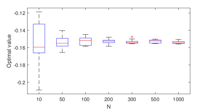
We have also studied the impact of the sample size of $s$ on the optimal value and optimal portfolio weights. We solve problem (6.2) via Algorithm 1 using training datasets of cardinality $K=100$ . The radius of the ambiguity set is fixed with $r=0.1$ , and the number of breakpoints is also fixed at $M=99$ . The sample size of $s$ varies with $N=10,50,100,200,300,500,1000$ . Figures 9 and 9 depict the convergence of the optimal portfolio weights $Z_{N}$ and the optimal value $\vartheta^{N}$ as the sample size $N$ increase. Figure 9 implies that the sequence of the optimal values $\vartheta^{N}$ converges.

Finally, we investigate impact of the radius $r$ of the Kantorovich ball on the out-of-sample performance of model (6.1). Specifically, for each $r$ , we obtain an optimal solution $z_{N}(r)$ from solving problem (6.1) and calculate check the change of ARSRM $\rho_{Q^{*}}(-z_{N}(r)^{\top}\xi)$ of $-z_{N}(r)^{\top}\xi$ using the true distribution $Q^{*}$ and compare it with ${\vartheta}_{N}$ . Since $Q^{*}$ is unknown, we generate validation data of size $3000$ to evaluate $\rho_{Q^{*}}(-z_{N}(r)^{\top}\xi)$ . For each fixed $r$ , we run 100 simulations with randomly generated training data of sample size $N=30$ . The blue shaded areas depict the tube of the optimal values ${\vartheta}_{N}$ between $20\%$ and $80\%$ quantiles. The solid black curve is the sample mean. For each simulation, we examine whether inequality $\rho_{Q^{*}}(-z_{N}(r)^{\top}\xi)\leq{\vartheta}_{N}$ holds or not, and count once if it holds and zero otherwise. The yellow depicts the percentages that the inequality holds out of 100 simulations when $r$ changes from $10^{-4}$ to $10^{0}$ . According to [12], this is called reliability. To explain the idea, observe that $\rho_{Q^{*}}(-z_{N}(r)^{\top}\xi)\geq{\vartheta}^{*}$ (where ${\vartheta}^{*}$ denotes the true ARSRM value) and inequality $\rho_{Q^{*}}(-z_{N}(r)^{\top}\xi)\leq{\vartheta}_{N}$ implies that ${\vartheta}^{*}\leq{\vartheta}_{N}$ . Thus, the more times the inequality holds, the more reliable that we may use ${\vartheta}_{N}$ as an upper bound of ${\vartheta}^{*}$ . The figure shows that when $r$ is increased to $10^{-1}$ , the reliability reaches $100\%$ which means that we do not need a large $r$ in this test.

6.3 Kusuoka’s representation

The second set of tests concerns model (5.1) with $\mathcal{M}$ being Kusouka’s ambiguity set. In this case, the true risk spectrum takes a form of $\sigma(t,\alpha)=\frac{1}{1-\alpha}\mathbbm{1}_{[\alpha,1]}(t)$ for $s\in(0,1)$ . To justify the application the model in this context, we assume that the portfolio manager’s risk preference can be described by $\int_{0}^{1}\mbox{\rm{CVaR}}_{\alpha}(\cdot)\mu(d\alpha)$ for some $\mu\in\mathscr{M}$ (see Assumption 3.1). Consequently the minmax optimization model can be formulated as

\min_{z\in Z}\quad\sup_{\mu\in\mathcal{M}}\int_{0}^{1}\mbox{\rm{CVaR}}_{\alpha}(-z^{\top}\xi)\mu(d\alpha).

Differing from the previous set of tests, we use pairwise comparison approach to construct the ambiguity set as outlined in Section 3.2. Let $\mathcal{M}_{pair}$ denote the ambiguity set. We consider the following program:

\min_{z\in Z}\sup_{\mu\in\mathcal{M}_{pair}}\int_{0}^{1}\mbox{\rm{CVaR}}_{\alpha}(-z^{\top}\xi)\mu(d\alpha),

(6.3)

As discussed in Section 4.2, we assume that $\alpha$ is discretely distributed with finite support over $(0,1)$ , i.e., $\mu(\alpha=\alpha_{i})=m_{i}$ for $i\in[N]$ . In addition, we assume that the true probability distribution of $\alpha$ , denoted by $\mu^{*}$ , satisfies $\mu^{*}(\alpha=\alpha_{i})=m^{*}_{i}$ for $i\in[N]$ .

6.3.1 Design of Kusuoka’s ambiguity set

We use the random relative utility split scheme (RRUS) considered by Armbruster and Delage [4] to design the questions. Specifically, we ask the investor questions comparing a risky lottery with two random outcomes and a certain lottery with deterministic outcome, denoted respectively by

Y_{1}=\left\{\begin{aligned} y_{1}\quad&\text{with \ probability $1-p$},\\ y_{3}\quad&\text{with \ probability \ $p$},\end{aligned}\right.\text{and}\ Y_{2}=y_{2}.

Each question is described by four parameters $y_{1}<y_{2}<y_{3}$ and a probability $p$ . Determine the number of questions $J$ . Below are the procedures.

Step 0

Set $j=0$ and ${\cal M}^{0}:=\{\bm{m}\in{\rm I\!R}_{+}^{N}:\sum_{i=1}^{N}m_{i}=1\}$ . For $j\leq J$ , do Steps 1-3.

Step 1

Generate two random numbers denoted by $y_{1}^{j}$ and $y_{3}^{j}$ and assume for the convenience of exposition that $y_{1}^{j}<y_{3}^{j}$ , let $p^{j}\in(0,1)$ be a positive number, which is randomly generated or designed. Define a lottery (a random variable $Y_{1}^{j}$ ) with outcomes $y_{1}^{j}$ and $y_{3}^{j}$ and respective probabilities $1-p^{j}$ and $p^{j}$ . The risk value of $Y_{1}^{j}$ can be expressed as

\begin{split}\rho(Y_{1}^{j})=&\sum_{i=1}^{N}m_{i}\mbox{\rm{CVaR}}_{\alpha_{i}}(Y_{1}^{j})\\ =&\sum_{i=1}^{N}m_{i}\left(\frac{y_{1}^{j}}{1-\alpha_{i}}\int_{0}^{1-p^{j}}\mathbbm{1}_{[\alpha_{i},1]}(t)dt+\frac{y_{3}^{j}}{1-\alpha_{i}}\int_{1-p^{j}}^{1}\mathbbm{1}_{[\alpha_{i},1]}(t)dt\right)\\ =&\sum_{i=1}^{N}m_{i}\left(y_{1}^{j}\phi_{i}(p^{j})+y_{3}^{j}\left(1-\phi_{i}(p^{j})\right)\right),\end{split}

where $\phi_{i}(p)=\frac{1}{1-\alpha_{i}}\int_{0}^{1-p}\mathbbm{1}_{[\alpha_{i},1]}(t)dt$ for $i\in[N]$ .

Step 2

Calculate

I_{u}:=\sup_{\bm{m}\in\mathcal{M}^{j}}\sum_{i=1}^{N}m_{i}\left(y_{1}^{j}\phi_{i}(p^{j})+y_{3}^{j}\left(1-\phi_{i}(p^{j})\right)\right)

and

I_{l}:=\inf_{\bm{m}\in\mathcal{M}^{j}}\sum_{i=1}^{N}m_{i}\left(y_{1}^{j}\phi_{i}(p^{j})+y_{3}^{j}\left(1-\phi_{i}(p^{j})\right)\right).

Let $y_{2}^{j}=\frac{1}{2}(I_{u}+I_{l})$ .

Step 3

If $\sum_{i=1}^{N}m^{*}_{i}\left(y_{1}^{j}\phi_{i}(p^{j})+y_{3}^{j}\left(1-\phi_{i}(p^{j})\right)\right)\leq y_{2}^{j}$ , then

\mathcal{M}^{j+1}:=\mathcal{M}^{j}\cap\left\{\bm{m}\in{\rm I\!R}_{+}^{N}:\sum_{i=1}^{N}m_{i}\left(y_{1}^{j}\phi_{i}(p^{j})+y_{3}^{j}\left(1-\phi_{i}(p^{j})\right)\right)\leq y_{2}^{j}\right\}.

Otherwise,

\mathcal{M}^{j+1}:=\mathcal{M}^{j}\cap\left\{\bm{m}\in{\rm I\!R}_{+}^{N}:\sum_{i=1}^{N}m_{i}\left(y_{1}^{j}\phi_{i}(p^{j})+y_{3}^{j}\left(1-\phi_{i}(p^{j})\right)\right)\geq y_{2}^{j}\right\}.

Let $j:=j+1$ . Go to Step 1.

In the $j$ th iteration, Step 1 generates a lottery with two random outcomes $y_{1}^{j}$ and $y_{3}^{j}$ and respective probabilities $1-p^{j}$ and $p^{j}$ ; Step 2 provides an approach of choosing a certain outcome $y_{2}^{j}$ , which can reduce the size of the ambiguity set efficiently when a new question is added; Step 3 asks the DM to choose between the lottery and the one with certain loss $y_{2}^{j}$ . Here the true RM defined as $\rho^{*}(\cdot):=\sum_{i=1}^{N}m_{i}^{*}\mbox{\rm{CVaR}}_{\alpha_{i}}(\cdot)$ is used to “act as the DM ”. After the DM makes a choice, a linear inequality is created and added to the ambiguity set $\mathcal{M}^{j}$ .

6.3.2 Tractable formulation of (6.3)

According to the construction of the Kusuoka’s ambiguity set outlined in Section 6.3.1, we can write down problem (6.3) as

\begin{split}\min_{z\in Z}\quad&\sup_{\bm{m}\in{\rm I\!R}_{+}^{N}}\sum_{i=1}^{N}m_{i}\mbox{\rm{CVaR}}_{\alpha_{i}}(-z^{\top}\xi)\\ \mbox{\rm{s.t.}}\quad&\sum_{i=1}^{N}m_{i}=1,\\ &\sum_{i=1}^{N}m_{i}\left(y_{1}^{j}\phi_{i}(p^{j})+y_{3}^{j}\left(1-\phi_{i}(p^{j})\right)\right)\leq y_{2}^{j},\ \forall\ j\in[J],\end{split}

(6.4)

and reformulate the latter via (5.5) and Lagrange duality as a single linear programming problem

$\displaystyle\min_{z\in Z,\eta,\bm{\lambda},\bm{\zeta}}\quad$	$\displaystyle\eta+\sum_{j=1}^{J}\lambda_{j}y_{2}^{j}$
s.t.	$\displaystyle\bm{\lambda}\geq 0,$	(6.5)
	$\displaystyle\zeta_{i}+\frac{1}{1-\alpha_{i}}\mathbb{E}\left[(-z^{\top}\xi-\zeta_{i})_{+}\right]\leq\eta+\sum_{j=1}^{J}\lambda_{j}\left(y_{1}^{j}\phi_{i}(p^{j})+y_{3}^{j}\left(1-\phi_{i}(p^{j})\right)\right),\ \forall i\in[N],$

where $\mathbb{E}[\cdot]$ denotes the expectation operator w.r.t. the probability distribution of $\xi$ .

6.3.3 Numerical results

In this set of tests, we pick up the elements of $\mathcal{A}=\{\alpha_{1},\cdots,\alpha_{N}\}$ randomly over $(0,1)$ , sort them in non-decreasing order, and set $\mu^{*}(\cdot)=\frac{1}{N}\sum_{i=1}^{N}\delta_{\alpha_{i}}(\cdot)$ . By using the relation $\sigma(t)=\int_{0}^{t}(1-\alpha)^{-1}\mu(d\alpha)$ (see Section 1), and the right-continuity of risk spectrum $\sigma$ , we have

\sigma(t)=\sum_{i=0}^{N}\sum_{\ell=0}^{i}\frac{\mu(\alpha=\alpha_{\ell})}{1-\alpha_{\ell}}\mathbbm{1}_{[\alpha_{i},\alpha_{i+1})}(t),

(6.6)

where $\alpha_{0}=0$ and $\alpha_{N+1}=1$ . In this case, $\sigma(t)$ is a step-like function with breakpoints $\mathcal{A}$ . We derive the worst-case $\mu(\alpha=\alpha_{i})$ for $i\in[N]$ by solving the optimization problem (6.3.2). To examine the effectiveness of the pairwise comparison approach outlined in Section 6.3.1, we use (6.6) to visualize our computational results by showing the corresponding step-like risk spectrum.

Figure 11 depicts the change of the optimal values of (6.3.2) as the number of questions increases. The decresing trend is because the feasible set of inner maximization problem is reduced as the number of questionnaires increases. Figure 11 depicts the corresponding optimal portfolio weights as the number of questions increases from $5$ to $100$ .

Figure 12 depicts the changes of the worst-case risk spectrum constructed by solving problem (6.3.2) and using the relation (6.6). The result of Figure 12 shows that the worst-case step-like risk spectrum becomes more and more approximate to the true one as the number of questionnaire increases.

7 Extensions

In the previous sections, we consider the case that the random risk spectra are step-like and the state variable is finitely distributed to facilitate preference elicitation and numerical computation of the randomized SRM models. In practice, the risk spectrum of a DM’s risk preference does not have to be step-like and also the state variable $s$ may be continuously distributed (which means the DM’s risk preferences cannot be described by a finite number of SRM). If we apply the established models to the general cases, where $\sigma(\cdot,s)$ is not step-like and $s$ is continuously distributed, then there will be inevitably modelling errors. In this section, we quantify the model errors so that we are guaranteed that the approximate models and computational schemes developed in the previous sections can be used within a prescribed precision.

7.1 Static step-like approximation

Let $Q^{*}$ be the true probability distribution of $s$ . We consider the following expected SRM minimization problem:

\displaystyle\vartheta^{*}:=\min_{z\in Z}\ \mathbb{E}_{Q^{*}}\left[\rho_{\sigma(\cdot,s)}\left(f(z,\xi)\right)\right],

(7.1)

where $\mathbb{E}_{Q^{*}}[\cdot]$ is the expectation value w.r.t. $Q^{*}$ , $\sigma(\cdot,s)\in\mathfrak{S}(S)\subseteq\mathscr{L}^{q}[0,1]$ and $q\in[1,\infty)$ . To ensure well-definiteness of (7.1), we make the following assumption.

Assumption 7.1

Let $\mathscr{G}_{f}:=\{F_{f(z,\xi)}^{\leftarrow}(\cdot):z\in Z\}$ . There exist a constant $p\in[1,\infty)$ with $\frac{1}{p}+\frac{1}{q}=1$ and a positive function $\psi_{f}\in\mathscr{L}^{p}[0,1]$ such that $\sup_{g\in\mathscr{G}_{f}}|g(t)|\leq\psi_{f}(t)$ and $\mathbb{E}_{Q}\left[\int_{0}^{1}\psi_{f}(t)\sigma(t,s)dt\right]$ $<\infty$ for any $Q\in\mathscr{P}(S)$ .

Without loss of generality, we assume that $\sigma(\cdot,s)$ is a general non-negative, non-decreasing function with the normalized property $\int_{0}^{1}\sigma(t,s)dt=1$ but it does not necessarily have a step-like structure. Let $\mathfrak{S}_{M}(S)$ denote the set of all non-negative, non-decreasing, and normalized step-like functions over $[0,1]$ with breakpoints $\{t_{1},\cdots,t_{M}\}$ , where $0<t_{1}<\cdots<t_{M}<1$ for all $s\in S$ and $S$ is a compact set. We consider the step-like approximation of $\sigma(\cdot,s)\in\mathfrak{S}(S)$ .

Definition 7.1

Let $\sigma(\cdot,s)\in\mathfrak{S}(S)$ . $\sigma_{M}(\cdot,s)$ is said to be a step-like approximation of $\sigma(\cdot,s)$ if $\sigma_{M}(t,s)=\sigma_{i}(s)$ , for $t\in[t_{i},t_{i+1})$ , $i\in[M_{0}]$ , such that $\sigma_{i}(s)\in[\sigma(t_{i},s),\sigma(t_{i+1},s)]$ , for $i\in[M_{0}]$ , and $\int_{0}^{1}\sigma_{M}(t,s)=\sum_{i=0}^{M}\sigma_{i}(s)(t_{i+1}-t_{i})=1$ .

We propose to obtain an approximate optimal value and optimal solution of problem (7.1) by solving the following step-like approximate ARSRM minimization problem:

\displaystyle\vartheta_{M}^{*}:=\min_{z\in Z}\ \mathbb{E}_{Q^{*}}\left[\rho_{\sigma_{M}(\cdot,s)}(f(z,\xi))\right].

(7.2)

Since $\mathfrak{S}_{M}(S)\subset\mathfrak{S}(S)$ , then $\mathbb{E}_{Q^{*}}\left[\rho_{\sigma_{M}(\cdot,s)}(f(z,\xi))\right]$ is well-defined under Assumption 7.1. Let $Z^{*}$ and $Z_{M}$ be the respective optimal solutions of problem (7.1) and (7.2). Let

\Delta_{M}:=\max_{i\in[M_{0}]}\left|t_{i+1}-t_{1}\right|.

(7.3)

It is obvious that in order to ensure approximate validity, we need $\Delta_{M}$ to be sufficiently small, which is equivalent to setting $M$ a large value.

Proposition 7.1 (Step-like approximation of random risk spectra)

Assume: (a) for each fixed $s\in S$ , $\sigma(\cdot,s)$ is Lipschitz continuous over $[0,1]$ with modulus $L(s)$ where $\mathbb{E}_{Q^{*}}[L(s)]<\infty$ and the expectation is taken w.r.t. the probability distribution of $s$ , (b) Assumption 7.1 holds and $\int_{0}^{1}\psi_{f}(t)dt<\infty$ . Let $\sigma_{M}(\cdot,s)$ denote a step-like approximation of $\sigma(\cdot,s)$ . Then the following assertions hold.

(

i

)

Let $\Delta_{M}$ be defined as in (7.3). Then

\displaystyle|\vartheta^{*}-\vartheta_{M}^{*}|\leq\mathbb{E}_{Q^{*}}\left[L(s)\right]\Delta_{M}\int_{0}^{1}\psi_{f}(t)dt.

(7.4)

( $ii$ )

Let $\{Z_{M}\}$ be a sequence of optimal solutions obtained form solving problem (7.2). Then every cluster point of the sequence is an optimal solution of problem (7.1), that is ,

$\displaystyle\lim_{M\rightarrow\infty}\mathbb{D}(Z_{M},Z^{*})=0,$ (7.5)

where $\mathbb{D}(A,B)$ denotes the access distance of set $A$ over set $B$ .

Proof. Part (i). Under Assumption 7.1, $\rho_{\sigma(\cdot,s)}(f(z,\xi))$ is finite-valued for each fixed $z\in Z$ . Under conditions (a) and (b),

\begin{split}\left|\rho_{\sigma(\cdot,s)}(f(z,\xi))-\rho_{\sigma_{M}(\cdot,s)}(f(z,\xi))\right|&=\left|\sum_{i=0}^{M}\int_{t_{i}}^{t_{i+1}}F_{f(z,\xi)}^{\leftarrow}(\sigma(t,s)-\sigma_{M}(t,s))dt\right|\\ &\leq\sum_{i=0}^{M}\int_{t_{i}}^{t_{i+1}}F_{f(z,\xi)}^{\leftarrow}|\sigma(t_{i+1},s)-\sigma(t_{i},s)|dt\\ &\leq\sum_{i=0}^{M}L(s)|t_{i+1}-t_{i}|\int_{t_{i}}^{t_{i+1}}\left|F_{f(z,\xi)}^{\leftarrow}(t)\right|dt\\ &\leq L(s)\Delta_{M}\int_{0}^{1}\psi_{f}(t)dt<\infty,\end{split}

where the first inequality follows from the definition of $\sigma_{M}(t,s)$ and the fact that $\sigma(t,s)$ is non-decreasing w.r.t. $t$ . Moreover, under Assumption 7.1, $\mathbb{E}_{Q^{*}}[\rho_{\sigma(\cdot,s)}(f(z,\xi))]$ is finite-valued. The discussions above imply that

\left|\mathbb{E}_{Q^{*}}[\rho_{\sigma(\cdot,s)}(f(z,\xi))]-\mathbb{E}_{Q^{*}}[\rho_{\sigma_{M}(\cdot,s)}(f(z,\xi))]\right|\leq\mathbb{E}_{Q^{*}}[L(s)]\Delta_{M}\int_{0}^{1}\psi_{f}(t)dt.

Furthermore, since $Z$ is compact and $\rho_{\sigma(\cdot,s)}(f(z,\xi))$ is continuous in $z$ for all $\sigma(\cdot,s)\in\mathfrak{S}(S)$ , then

\begin{split}|\vartheta^{*}-\vartheta_{M}^{*}|&\leq\sup_{z\in Z}\left|\mathbb{E}_{Q^{*}}[\rho_{\sigma(\cdot,s)}(f(z,\xi))]-\mathbb{E}_{Q^{*}}[\rho_{\sigma_{M}(\cdot,s)}(f(z,\xi))]\right|\\ &\leq\mathbb{E}_{Q^{*}}[L(s)]\Delta_{M}\int_{0}^{1}\psi_{f}(t)dt.\end{split}

Part (ii) follows directly from Part (i) and the well-known stability results in parametric programming [24, Lemma 3.8].

Note that the conclusion of Proposition 7.1 depends heavily on the assumption that $\sigma(\cdot,s)$ is Lipschitz continuous, which excludes many unbounded risk spectra such as Wang’s risk spectrum. In the case when $\sigma(\cdot,s)$ is not Lipschtz continuous, one may set the breakpoints in a specific way such that the following assumption is satisfied, we refer readers to [35, Section 4.1] for a thorough discussion on this.

7.2 Discretization of the state variable

The computational schemes discussed in Section 6 rely on the discrete distribution of $s$ . In practice, the true probability distribution of $s$ may be unknown, but by can be estimated using sample data. Let $s^{1},\cdots,s^{N}$ denote i.i.d random sampling of $s$ and $Q_{N}=\frac{1}{N}\sum_{i=1}^{N}\delta_{s^{i}}(\cdot)$ , where $\delta_{s^{i}}(\cdot)$ denotes the Dirac probability measure at $s^{i}$ . We propose to approximate the true mean value of $\rho_{\sigma(\cdot,s)}(f(z,\xi))$ , i.e., $\mathbb{E}_{Q^{*}}[\rho_{\sigma(\cdot,s)}(f(z,\xi))]$ , using the sample average

\mathbb{E}_{Q_{N}}\left[\rho_{\sigma_{M}(\cdot,s)}(f(z,\xi))\right]=\frac{1}{N}\sum_{i=1}^{N}\rho_{\sigma_{M}(\cdot,s^{i})}(f(z,\xi)).

The next proposition gives a quantification of such an approximation.

Proposition 7.2 (Sample average approximation of $s$ )

Assume the settings and conditions of Proposition 7.1. For any $\varepsilon>0$ and $\theta>0$ , let $N_{0}:=-\frac{\ln\theta}{\Upsilon(\varepsilon)}$ . Then

\displaystyle{\rm{Prob}}\left(\min_{z\in Z}\left|\mathbb{E}_{Q_{N}}\left[\rho_{\sigma_{M}(\cdot,s)}(f(z,\xi))\right]-\mathbb{E}_{Q^{*}}\left[\rho_{\sigma(,s)}(f(z,\xi))\right]\right|\geq\varepsilon\right)\leq\theta

(7.6)

for all $N\geq N_{0}$ and $\Delta_{M}\leq\frac{\varepsilon}{2\mathbb{E}[L(s)]\int_{0}^{1}\psi_{f}(t)dt}$ , where $\mathbb{E}[\cdot]$ is the expectation w.r.t. the true distribution $Q^{*}$ of $s$ .

Proof. By the triangle inequality, we have

\begin{split}&\left|\mathbb{E}_{Q_{N}}[\rho_{\sigma_{M}(\cdot,s)}(f(z,\xi))]-\mathbb{E}_{Q^{*}}[\rho_{\sigma(\cdot,s)}(f(z,\xi))]\right|\\ &\leq|\mathbb{E}_{Q_{N}}[\rho_{\sigma_{M}(\cdot,s)}(f(z,\xi))]-\mathbb{E}_{Q^{*}}[\rho_{\sigma_{M}(\cdot,s)}(f(z,\xi))]|\\ &\ \ \ +|\mathbb{E}_{Q^{*}}[\rho_{\sigma_{M}(\cdot,s)}(f(z,\xi))]-\mathbb{E}_{Q^{*}}[\rho_{\sigma(\cdot,s)}(f(z,\xi))].|\end{split}

By Proposition 7.1, we have

\left|\mathbb{E}_{Q^{*}}[\rho_{\sigma(\cdot,s)}(f(z,\xi))]-\mathbb{E}_{Q^{*}}[\rho_{\sigma_{M}(\cdot,s)}(f(z,\xi))]\right|\leq\mathbb{E}_{Q^{*}}[L(s)]\Delta_{M}\int_{0}^{1}\psi_{f}(t)dt.

(7.7)

Let $\Delta_{M}$ be sufficiently small such that $\mathbb{E}_{Q^{*}}[L(s)]\Delta_{M}\int_{0}^{1}\psi_{f}(t)dt\leq\frac{\varepsilon}{2}$ , i.e., $\Delta_{M}\leq\frac{\varepsilon}{2\mathbb{E}_{Q^{*}}[L(s)]\int_{0}^{1}\psi_{f}(t)dt}$ . By (7.7)

\begin{split}&\min_{z\in Z}\left|\mathbb{E}_{Q_{N}}[\rho_{\sigma_{M}(\cdot,s)}(f(z,\xi))]-\mathbb{E}_{Q^{*}}[\rho_{\sigma(,s)}(f(z,\xi))]\right|\\ \leq&\sup_{z\in Z}\left|\mathbb{E}_{Q_{N}}[\rho_{\sigma_{M}(\cdot,s)}(f(z,\xi))]-\mathbb{E}_{Q^{*}}[\rho_{\sigma_{M}(\cdot,s)}(f(z,\xi))]\right|\\ &\ +\sup_{z\in Z}\left|\mathbb{E}_{Q^{*}}[\rho_{\sigma_{M}(\cdot,s)}(f(z,\xi))]-\mathbb{E}_{Q^{*}}[\rho_{\sigma(\cdot,s)}(f(z,\xi))]\right|\\ \leq&\sup_{z\in Z}\left|\mathbb{E}_{Q_{N}}[\rho_{\sigma_{M}(\cdot,s)}(f(z,\xi))]-\mathbb{E}_{Q^{*}}[\rho_{\sigma_{M}(\cdot,s)}(f(z,\xi))]\right|+\frac{\varepsilon}{2}.\end{split}

(7.8)

Moreover,

\begin{split}&\left|\mathbb{E}_{Q_{N}}[\rho_{\sigma_{M}(\cdot,s}(f(z,\xi))]-\mathbb{E}_{Q^{*}}[\rho_{\sigma_{M}(\cdot,s)}(f(z,\xi))]\right|\\ =&\left|\frac{1}{N}\sum_{j=1}^{N}\left[\sum_{i=0}^{M}\int_{t_{i}}^{t_{i+1}}\sigma_{i}(s^{j})F_{f(z,\xi)}^{\leftarrow}(t)dt\right]-\mathbb{E}_{Q^{*}}\left[\sum_{i=0}^{M}\sigma_{i}(s)\int_{t_{i}}^{t_{i+1}}F_{f(z,\xi)}^{\leftarrow}(t)dt\right]\right|\\ =&\left|\sum_{i=0}^{M}\left(\mathbb{E}_{Q_{N}}[\sigma_{i}(s)]-\mathbb{E}_{Q^{*}}[\sigma_{i}(s)]\right)\int_{t_{i}}^{t_{i+1}}F^{\leftarrow}_{f(z,\xi)}(t)dt\right|\\ \leq&\max_{i\in[M_{0}]}\left|\mathbb{E}_{Q_{N}}[\sigma_{i}(s)]-\mathbb{E}_{Q^{*}}[\sigma_{i}(s)]\right|\int_{0}^{1}\left|F_{f(z,\xi)}^{\leftarrow}(t)\right|dt\\ \leq&\|\mathbb{E}_{Q_{N}}\left[\bm{\sigma(s)}]-\mathbb{E}_{Q^{*}}[\bm{\sigma(s)}\right]\|_{\infty}\int_{0}^{1}\psi_{f}(t)dt,\\ \end{split}

(7.9)

where $\bm{\sigma(s)}=(\sigma_{0}(s),\sigma_{1}(s),\cdots,\sigma_{M}(s))^{\top}$ and $\|\cdot\|_{\infty}$ denotes the infinity norm in ${\rm I\!R}^{M+1}$ . Combining (7.8) and (7.9), we obtain

\begin{split}&{\rm{Prob}}\left(\min_{z\in Z}|\mathbb{E}_{Q_{N}}\rho_{\sigma_{M}(\cdot,s)}(f(z,\xi))-\mathbb{E}_{Q^{*}}[\rho_{\sigma(,s)}(f(z,\xi))]|\geq\varepsilon\right)\\ \leq&{\rm{Prob}}\left(\|\mathbb{E}_{Q_{N}}[\bm{\sigma(s)}]-\mathbb{E}_{Q^{*}}[\bm{\sigma(s)}]\|_{\infty}\int_{0}^{1}\psi_{f}(t)dt\geq\frac{\varepsilon}{2}\right).\end{split}

Recall that the condition (b) of Proposition 7.1 ensures that $\int_{0}^{1}\psi_{f}(t)dt<\infty$ . Thus by Cram $\acute{e}$ r’s large deviation theorem, there exists a positive integer $N_{0}$ and positive constant $\Upsilon(\varepsilon)$ (depending on $\varepsilon$ with $\Upsilon(0)=0$ ) such that for all $N\geq N_{0}$

{\rm{Prob}}\left(\|\mathbb{E}_{Q_{N}}[\bm{\sigma(s)}]-\mathbb{E}_{Q^{*}}[\bm{\sigma(s)}]\|_{\infty}\int_{0}^{1}\psi_{f}(t)dt\geq\frac{\varepsilon}{2}\right)\leq e^{-\Upsilon(\varepsilon)N}.

For fixed $\theta\in(0,1)$ , we let $N_{0}(\varepsilon,\theta):=-\frac{\ln\theta}{\Upsilon(\varepsilon)}$ and subsequently obtain

{\rm{Prob}}\left(\|\mathbb{E}_{Q_{N}}[\bm{\sigma(s)}]-\mathbb{E}_{Q^{*}}[\bm{\sigma(s)}]\|_{\infty}\int_{0}^{1}\psi_{f}(t)dt\geq\frac{\varepsilon}{2}\right)\leq\theta

for all $N\geq N_{0}(\varepsilon,\theta)$ .

7.3 Error bounds for the step-like approximation and discretization

Consider minimax optimization problem (5.1) with the Kantorovich ambiguity set $\mathfrak{Q}^{V}_{K}(Q_{V},r)$ , which contains only discrete distributions:

\vartheta_{M}^{V}:=\min_{z\in Z}\sup_{Q\in\mathfrak{Q}^{V}_{K}(Q_{V},r)}\mathbb{E}_{Q}[\rho_{\sigma_{M}(\cdot,s)}(f(z,\xi))],

(7.10)

where

\displaystyle\mathfrak{Q}^{V}_{K}(Q_{V},r):=\{Q\in\mathscr{P}(\mathcal{S}^{V}):\mathsf{dl}_{K}(Q,Q_{V})\leq r\},

(7.11)

$Q_{V}$ is defined as in (3.4). Let $\mathfrak{Q}_{K}(Q_{N},r)$ be the counterpart of $\mathfrak{Q}^{V}_{K}(Q_{V},r)$ which contains both discrete and continuous distributions in the ball and

\vartheta_{M}^{N}:=\min_{z\in Z}\sup_{Q\in\mathfrak{Q}_{K}(Q_{N},r)}\mathbb{E}_{Q}[\rho_{\sigma_{M}(\cdot,s)}(f(z,\xi))].

We want to quantify the difference between ${\vartheta}_{M}^{V}$ and $\vartheta_{M}^{N}$ . Let

\mathfrak{F}:=\{h(\cdot):=\int_{0}^{1}F^{\leftarrow}_{f(z,\xi)}(t)\sigma_{M}(t,\cdot)dt,\ \forall z\in Z\},

and for any two probability measures $Q_{1},Q_{2}\in\mathscr{P}(S)$ , define pseudo-metric

\mathsf{dl}_{\mathfrak{F}}(Q_{1},Q_{2}):=\sup_{z\in Z}\left|\mathbb{E}_{Q_{1}}\left[\int_{0}^{1}F^{\leftarrow}_{f(z,\xi)}(t)\sigma_{M}(t,s_{1})dt\right]-\mathbb{E}_{Q_{2}}\left[\int_{0}^{1}F^{\leftarrow}_{f(z,\xi)}(t)\sigma_{M}(t,s_{2})dt\right]\right|,

where $s_{1}$ and $s_{2}$ follow distributions $Q_{1}$ and $Q_{2}$ respectively. For any two sets of probability measures $\mathfrak{Q}_{1}$ and $\mathfrak{Q}_{2}$ , let $\mathbb{H}_{\mathfrak{F}}(\mathfrak{Q}_{1},\mathfrak{Q}_{2})$ denote the Hausdorff distance between the two sets under the pseudo-metric $\mathsf{dl}_{\mathfrak{F}}(Q_{1},Q_{2})$ .

Next, we quantify the difference between ${\vartheta}^{*}$ and ${\vartheta}_{M}^{N}$ . We need the following assumption.

Assumption 7.2

For each $\sigma(\cdot,s)\in\mathfrak{S}(S)$ , its step-like approximation, $\sigma_{M}(\cdot,s)$ , is Lipschitz continuous in $s$ over $S$ , i.e., for any fixed $t\in[0,1]$ , there exists a positive constant $L$ such that $\|\sigma_{M}(t,s_{1})-\sigma_{M}(t,s_{2})\|\leq L\|s_{1}-s_{2}\|$ for all $s_{1},s_{2}\in S$ .

To see how the assumption may be possibly satisfied, we take a look at the randomized risk spectra in Example 2.1. Consider $\sigma(t,\alpha)$ defined in (2.1). The function is step-like with breakpoint $\alpha$ . In this case, any step-like approximation of the function is discontinuous in $\alpha$ . Thus the Lipschitz condition fails to hold in this case. Next, consider (2.3). The step-like approximation of $\sigma(\cdot,s)$ onto the space $\mathfrak{S}_{M}((0,1])$ can be written as:

\sigma_{M}(t,s)=\left\{\begin{array}[]{lcl}\sigma(t_{i},s),&&\mbox{\rm{for}}\;t\in[t_{i},t_{i+1}),i\in[M_{0}]\backslash\{M\},\\ M+1-\sum_{i=0}^{M-1}\sigma(t_{i},s),&&\mbox{\rm{for}}\;t\in[t_{M},1),\end{array}\right.

where $\{t_{1},\cdots,t_{M}\}=\{1/(M+1),\cdots,M/(M+1)\}$ . It is easy to drive that for any $s_{1},s_{2}\in(0,1]$ and $M\geq 2$ ,

|\sigma_{M}(t,s_{1})-\sigma_{M}(t,s_{2})|\leq\left\{\begin{array}[]{lcl}\left(M+1)(\ln(M+1)-1\right)|s_{1}-s_{2}|,&&\mbox{\rm{for}}\;t\in[0,t_{M}),\\ M(M+1)(\ln(M+1)-1)|s_{1}-s_{2}|,&&\mbox{\rm{for}}\;t\in[t_{M},1).\end{array}\right.

Finally, consider (2.4). Since $|\sigma(t,s_{1})-\sigma(t,s_{2})|\leq|s_{1}-s_{2}|$ for all $t\in[0,1]$ , it is easy to verify that its step-like approximation onto the space $\mathfrak{S}_{M}([0,1])$ is also Lipschtz continuous w.r.t. $s$ with modulus $1$ .

We are now ready to state the main result of this section.

Theorem 7.1

Assume the settings and conditions of Proposition 7.1. Assume, in addition, that (a) Assumption 7.2 holds, (b) there exist positive constants $C$ , $v$ , and $\delta_{0}$ such that $Q^{*}(|s-s_{0}|\leq\delta)>C\delta^{v}$ for any fixed point $s_{0}\in S$ and $\delta\in(0,\delta_{0})$ , where $Q^{*}$ is a true continuous distribution of $s$ . Then for any $\theta\in(0,1)$ and $r=r_{N}(\theta)$ , there exist positive constants $V_{0}$ and $N_{0}$ such that

\displaystyle\vartheta^{*}\in[\vartheta_{M}^{V}-3L\Psi r_{N}(\theta),\vartheta_{M}^{V}+3L\Psi r_{N}(\theta)]

(7.12)

with probability at least $1-\theta$ for all $V\geq V_{0}$ , $N\geq N_{0}$ , where $\Psi=\int_{0}^{1}\psi_{f}(t)dt$ , $r_{N}(\theta)$ is defined as in (3.3) and $r_{N}(\theta)\leq 1$ ,

V_{0}=-\frac{\ln\left(\theta/(2\varrho_{1}(3L\Psi r_{N}(\theta)))\right)}{\varrho_{2}(3L\Psi r_{N}(\theta))},\ N_{0}=\max\left\{\frac{\log(C_{1}\theta^{-1})}{C_{2}r_{N}^{2}(\theta)},-\frac{\ln(\theta/2)}{\Upsilon(3L\Psi r_{N}(\theta)}\right\}

and $\Delta_{M}\leq\frac{3Lr_{N}(\theta)}{2\mathbb{E}[L(s)]}$ .

Proof. Under Assumption 7.2, we can derive the Lipschitz continuity of $\rho_{\sigma_{M}(\cdot,s)}(f(z,\xi))$ in $s$ , that is,

\begin{split}\left|\rho_{\sigma_{M}(\cdot,s_{1})}(f(z,\xi))-\rho_{\sigma_{M}(\cdot,s_{2})}(f(z,\xi))\right|=&\left|\sum_{i=0}^{M}(\sigma_{i}(s_{1})-\sigma_{i}(s_{2}))\int_{t_{i}}^{t_{i+1}}F^{\leftarrow}_{f(z,\xi)}(t)dt\right|\\ \leq&\max_{i\in[M_{0}]}|\sigma_{i}(s_{1})-\sigma_{i}(s_{2})|\int_{0}^{1}\psi_{f}(t)dt\leq L\Psi|s_{1}-s_{2}|\end{split}

where $\Psi=\int_{0}^{1}\psi_{f}(t)dt$ . By the definition of the Kantorovich metric, the Lipschitz continuity ensures that for any $Q\in\mathscr{P}(S)$

\displaystyle\left|\mathbb{E}_{Q}[\rho_{\sigma_{M}(\cdot,s)}(f(z,\xi))]-\mathbb{E}_{Q_{N}}[\rho_{\sigma_{M}(\cdot,s)}\left(f(z,\xi)\right)]\right|\leq L\Psi\mathsf{dl}_{K}(Q,Q_{N}).

(7.13)

By virtue of [29, Theorem 3] and [7, Theorem 2],

\begin{split}\left|\vartheta_{M}^{V}-\vartheta_{M}^{N}\right|&\leq\mathbb{H}_{\mathfrak{F}}\left(\mathfrak{Q}_{K}\left(Q_{N},r\right),\mathfrak{Q}_{K}^{V}\left(Q_{V},r\right)\right)\\ &\leq L\Psi\mathbb{H}_{K}\left(\mathfrak{Q}_{K}\left(Q_{N},r\right),\mathfrak{Q}_{K}^{V}\left(Q_{V},r\right)\right)\leq 3L\Psi\beta_{V},\end{split}

where $\beta_{V}=\max_{s\in S}\min_{1\leq j\leq V}d(s,\hat{s}^{j}),$ and $d(s,\hat{s}^{j})=\|s-\hat{s}^{j}\|$ denotes some norm distance in the Euclidean space. Note that $\beta_{V}$ depends on the selection of $\{\hat{s}^{1},\cdots,\hat{s}^{V}\}$ , thus $\beta_{V}$ is a random variable. By the triangle inequality

\begin{split}{\rm{Prob}}(|\vartheta_{M}^{V}-\vartheta^{*}|\geq\varepsilon)\leq&{\rm{Prob}}\left(\left(\left|\vartheta_{M}^{V}-\vartheta_{M}^{N}\right|+\left|\vartheta_{M}^{N}-\vartheta^{*}\right|\right)\geq\varepsilon\right)\\ \leq&{\rm{Prob}}\left(3L\Psi\beta_{V}\geq\frac{\varepsilon}{3}\right)+{\rm{Prob}}\left(\left|\vartheta_{M}^{N}-\vartheta^{*}\right|\geq\frac{2\varepsilon}{3}\right)\\ \leq&{\rm{Prob}}\left(\beta_{V}\geq\frac{\varepsilon}{9L\Psi}\right)+{\rm{Prob}}\left(\left|\vartheta_{M}^{N}-\vartheta^{*}\right|\geq\frac{2\varepsilon}{3}\right).\end{split}

(7.14)

for any small real number $\varepsilon>0$ . In the following, we show that there exist constants $V_{0}$ , $N_{0}$ and $M_{0}$ such that ${\rm{Prob}}\left(\beta_{V}\geq\frac{\varepsilon}{9L\Psi}\right)\leq\frac{\theta}{2}$ and ${\rm{Prob}}\left(\left|\vartheta_{M}^{N}-\vartheta^{*}\right|\geq\frac{2\varepsilon}{3}\right)\leq\frac{\theta}{2}$ for all $V\geq V_{0}$ , $N\geq N_{0}$ and $M\geq M_{0}$ . We proceed the rest of the proof in two steps.

Step 1. Since the support set $S$ of $s$ is bounded and the condition (b) holds, then it follows by [2], [38, Lemma 3.1] and [25, Proposition 9] that there exist positive constants $\varrho_{1}(\varepsilon)$ and $\varrho_{2}(\varepsilon)$ depending on $\varepsilon$ such that

{\rm{Prob}}\left(\beta_{V}\geq\frac{\varepsilon}{9L\Psi}\right)\leq\varrho_{1}(\varepsilon)e^{-\varrho_{2}(\varepsilon)N}.

Let $V_{0}:=-\frac{\ln\left(\theta/(2\varrho_{1}(\varepsilon))\right)}{\varrho_{2}(\varepsilon)}$ be such that ${\rm{Prob}}\left(\beta_{V}\geq\frac{\varepsilon}{9L\Psi}\right)\leq\frac{\theta}{2}$ for all $V\geq V_{0}$ .

Step 2. For each fixed $z\in Z$ and $Q\in\mathfrak{Q}_{K}(Q_{N},r)$ ,

\begin{split}\left|\mathbb{E}_{Q}[\rho_{\sigma_{M}(\cdot,s)}(f(z,\xi))]-\mathbb{E}_{Q^{*}}[\rho_{\sigma(\cdot,s)}(f(z,\xi))]\right|\leq&\left|\mathbb{E}_{Q}[\rho_{\sigma_{M}(\cdot,s)}(f(z,\xi))]-\mathbb{E}_{Q_{N}}[\rho_{\sigma_{M}(\cdot,s)}(f(z,\xi))]\right|\\ &+\left|\mathbb{E}_{Q_{N}}[\rho_{\sigma_{M}(\cdot,s)}(f(z,\xi))]-\mathbb{E}_{Q^{*}}[\rho_{\sigma(\cdot,s)}(f(z,\xi))]\right|.\end{split}

Let $E$ denote the event that $\mathsf{dl}_{K}(Q^{*},Q_{N})\leq r_{N}(\theta)$ for $r_{N}(\theta)\leq 1$ and $F$ denote the event that

\displaystyle\left|\mathbb{E}_{Q_{N}}[\rho_{\sigma_{M}(\cdot,s)}(f(z,\xi))]-\mathbb{E}_{Q^{*}}[\rho_{\sigma(\cdot,s)}(f(z,\xi))]\right|\leq\frac{\varepsilon}{3}.

(7.15)

By (3.2), (3.3) and Proposition 7.2, there exists a positive integer $N_{1}:=\max\left\{\frac{\log(2C_{1}\theta^{-1})}{C_{2}},-\frac{\ln(\theta/2)}{\Upsilon(\varepsilon)}\right\}$ and $M_{0}$ such that ${\rm{Prob}}(E\cap F)\geq 1-\frac{\theta}{2}$ and $\Delta_{M}\leq\frac{\varepsilon}{2\mathbb{E}[L(s)]\Psi}$ for all $N\geq N_{2}$ and $M\geq M_{0}$ . Consequently

	$\displaystyle{\rm{Prob}}\left(\left\|\vartheta_{M}^{N}-\vartheta^{*}\right\|\geq\frac{2\varepsilon}{3}\right)$	(7.16)
$\displaystyle\leq$	$\displaystyle{\rm{Prob}}\left(\sup_{z\in Z,Q\in\mathfrak{Q}_{K}(Q_{N},r)}\left\|\mathbb{E}_{Q}[\rho_{\sigma_{M}(\cdot,s)}(f(z,\xi))]-\mathbb{E}_{Q^{*}}[\rho_{\sigma(\cdot,s)}(f(z,\xi))]\right\|\geq\frac{2\varepsilon}{3}\right)$
$\displaystyle=$	$\displaystyle{\rm{Prob}}\left(\sup_{z\in Z,Q\in\mathfrak{Q}_{K}(Q_{N},r)}\left\|\mathbb{E}_{Q}[\rho_{\sigma_{M}(\cdot,s)}(f(z,\xi))]-\mathbb{E}_{Q^{*}}[\rho_{\sigma(\cdot,s)}(f(z,\xi))]\right\|\geq\frac{2\varepsilon}{3}\bigcap(E\cap F)\right)$
	$\displaystyle+{\rm{Prob}}\left(\sup_{z\in Z,Q\in\mathfrak{Q}_{K}(Q_{N},r)}\left\|\mathbb{E}_{Q}[\rho_{\sigma_{M}(\cdot,s)}(f(z,\xi))]-\mathbb{E}_{Q^{*}}[\rho_{\sigma(\cdot,s)}(f(z,\xi))]\right\|\geq\frac{2\varepsilon}{3}\bigcap(\overline{E\cap F})\right)$
$\displaystyle\leq$	$\displaystyle{\rm{Prob}}\left(\sup_{z\in Z,Q\in\mathfrak{Q}_{K}(Q_{N},r)}\left(\left\|\mathbb{E}_{Q}[\rho_{\sigma_{M}(\cdot,s)}(f(z,\xi))]-\mathbb{E}_{Q_{N}}[\rho_{\sigma_{M}(\cdot,s)}(f(z,\xi))]\right\|\right.\right.$
	$\displaystyle\left.\left.+\left\|\mathbb{E}_{Q_{N}}[\rho_{\sigma_{M}(\cdot,s)}(f(z,\xi))]-\mathbb{E}_{Q^{*}}[\rho_{\sigma(\cdot,s)}(f(z,\xi))]\right\|\right)\geq\frac{2\varepsilon}{3}\|E\cap F\right){\rm{Prob}}(E\cap F)+{\rm{Prob}}(\overline{E\cap F})$
$\displaystyle\leq$	$\displaystyle{\rm{Prob}}\left(\sup_{z\in Z,Q\in\mathfrak{Q}_{K}(Q_{N},r_{N}(\theta))}\left\|\mathbb{E}_{Q}[\rho_{\sigma_{M}(\cdot,s)}(f(z,\xi))]-\mathbb{E}_{Q_{N}}[\rho_{\sigma_{M}(\cdot,s)}(f(z,\xi))]\right\|\geq\frac{\varepsilon}{3}\right){\rm{Prob}}(E\cap F)$
	$\displaystyle\quad\quad+\frac{\theta}{2}$
$\displaystyle\leq$	$\displaystyle{\rm{Prob}}\left(\sup_{Q\in\mathfrak{Q}_{K}(Q_{N},r_{N}(\theta))}L\Psi\mathsf{dl}_{K}(Q,Q_{N})\geq\frac{\varepsilon}{3}\right)+\frac{\theta}{2},$

where the second last inequality results from (7.15) and the last inequality is due to (7.13). Let $N_{2}:=\frac{9L^{2}\Psi^{2}\log(C_{1}\theta^{-1})}{C_{2}\varepsilon^{2}}$ . Then $r_{N}(\theta)<\frac{\varepsilon}{3L\Psi}$ , i.e., $\varepsilon>3L\Psi r_{N}(\theta)$ for all $N\geq N_{2}$ . Summarizing the discussions above, we conclude that there exist $V_{0}:=\frac{\ln\left(\theta/(2\varrho_{1}(\varepsilon))\right)}{\varrho_{2}(\varepsilon)}$ , $N_{0}:=\max\left\{N_{1},N_{2}\right\}$ and $M_{0}$ such that

\begin{split}{\rm{Prob}}(|\vartheta_{M}^{V}-\vartheta^{*}|\geq\varepsilon)\leq&{\rm{Prob}}\left(\beta_{V}\geq\frac{\varepsilon}{9L\Psi}\right)+{\rm{Prob}}\left(\sup_{Q\in\mathfrak{Q}_{K}(Q_{N},r_{N}(\theta))}\mathsf{dl}_{K}(Q,Q_{N})>r_{N}(\theta)\right)+\frac{\theta}{2}\\ \leq&\frac{\theta}{2}+\frac{\theta}{2}=\theta\end{split}

for all $V\geq V_{0}$ , $N\geq N_{0}$ and $M\geq M_{0}$ . The inequality implies that

\vartheta^{*}\in[\vartheta_{M}^{V}-3L\Psi r_{N}(\theta),\vartheta_{M}^{V}+3L\Psi r_{N}(\theta)]

with probability at least $1-\theta$ for all $V\geq V_{0}$ , $N\geq N_{0}$ and $M\geq M_{0}$ .

8 Concluding remarks

In this paper, we explore randomization of spectral risk measure for the case that a single SRM does not exist for the description of a DM’s risk preferences. Differing from Bertsimas and O’Hair’s method [6] for tackling DM’s preference inconsistency where the authors regard inconsistencies as “mistakes” and consequently propose a remedy by relaxing the model to accommodate the mistakes so long as the total quantity of mistakes is controlled, we allow unlimited number of inconsistencies/mistakes. As such, the proposed model may be more easily utilized for descriptive analysis where the empirical data used to describe a DM’s past behaviour. It can perhaps also be more realistically used for prescriptive analysis by a modeller who does not have complete information on the DM’s risk preference and consequently uses the available data to forecast the DM’s future decisions. Moreover, the randomization of risk measures enables us to interpret the Kusuoka’s representation and spectral risk representation (1.2) of a law invariant risk measure from risk preference perspective and provide an avenue to construct an approximation of the ambiguity sets in these representations via preference elicitation. As we can see, the randomization depends on the “building blocks”, e.g., VaRs, or CVaRs or SRMs. We envisage that this kind of randomization approaches can be extended to other risk measures. Moreover, it will be interesting to investigate how to “learn” efficiently the DM’s preferences in terms of the type of $\sigma(\cdot,s)$ and the distribution of $s$ in practical applications. We leave all these for future research.

References

[1] Acerbi C.: Spectral measures of risk: A coherent representation of subjective risk aversion. J. Bank Financ. 26(7), 1505–1518 (2002)
[2] Anderson, E., Xu, H., Zhang, D.: Varying confidence levels for CVaR risk measures and minimax limits. Math. Program. 180(1), 327–370 (2020)
[3] Anscombe, F. J. and Aumann, R. J., A definition of subjective probability. Annals of Mathematical Statistics. 34(1):199–205 (1963)
[4] Armbruster, B., Delage, E.: Decision making under uncertainty when preference information is incomplete. Manag. Sci. 61(1), 111–-128 (2015)
[5] Artzner, P., Delbaen, F., Eber, J.M., Health, D.: Coherent measures of risk. Math. Finance 9, 203–228(1999)
[6] Bertsimas,D., O’Hair, A.: Learning preferences under noise and loss aversion: An optimization approach. Oper. Res. 61, 1190–1199 (2013)
[7] Chen. Y., Sun. H., Xu. H.: Decomposition and discrete approximation methods for solving two-stage distributionally robust optimization problems. Comput. Optim. Appl. 78(1), 205–238 (2021)
[8] Delage, E., Ye, Y.: Distributionally robust optimization under moment uncertainty with application to data-driven problems. Oper. Res. 58, 595–612 (2010)
[9] Delage, E., Kuhn, D., Wiesemann, W.: ”Dice”-sion–making under uncertainty: When can a random decision reduce risk?. Manag. Sci. 65(7), 3282–3301 (2019)
[10] Denneberg, D.: Premium calculation: why standard deviation should be replaced by absolute deviation. ASTIN Bulletin: The Journal of the IAA, 20(2):181–190 (1990)
[11] Dentcheva D, Ruszczyński A (2020) Risk forms: representation, disintegration, and application to partially observable two-stage systems. Math. Program. 181(2):297–317.
[12] Mohajerin, E.P., Kuhn, D.: Data-driven distributionally robust optimization using the Wasserstein metric: performance guarantees and tractable reformulations. Math. Program. 171, 115–166 (2018)
[13] Escobar, D., Pflug, G.: The distortion principle for insurance pricing: properties, identification and robustness. Ann. Oper. Res. 292(2), 771–-94, (2020)
[14] Fishburn, P. C.: Stochastic utility. In Barbera, S., Hammond, P. J., and Seidl, C., editors, Handbook of Utility Theory, volume 1, pages 273–320. Kluwer Academic Publishers, Boston, MA (1998)
[15] Fournier, N., Guillin, A.: On the rate of convergence in wasserstein distance of the empirical measure. Probab. Theory Relat. Fields 162(3), 707–738 (2015)
[16] Gao, R.: Finite-sample guarantees for Wasserstein distributionally robust optimization: Breaking the curse of dimensionality. Oper. Res. (2022)
[17] Goh, J., Sim, M.: . Distributionally robust optimization and its tractable approximations. Oper. Res. 58(4-part-1), 902–917 (2010)
[18] Guo, S., Xu, H.: Distributionally robust shortfall risk optimization model and its approximation. Math. Program. 174, 473–498 (2019)
[19] Guo, S., Xu, H.: Robust spectral risk optimization when the subjective risk aversion is ambiguous: a moment-type approach. Math. Program. 194(1), 305–340 (2022)
[20] Hu, J., Zhang, D., Xu, H., Zhang, S.: Distributionally Preference Robust Optimization in Multi-Attribute Decision Making. arXiv preprint arXiv:2206.04491 (2022)
[21] Koppen, M.: Characterization Theorems in Random Utility theory. In Smelser, N. J. and Baltes, P. B., editors, International Encyclopedia of the Social & Behavioral Sciences. Pergamon, Oxford. 1646–1651, 2001.
[22] Kusuoka, S.: On law invariant coherent risk measures, in Advances in mathematical economics, pp. 83–95, Springer, 2001.
[23] Lam, H.: Recovering best statistical guarantees via the empirical divergence-based distributionally robust optimization. Oper. Res. 67(4):1090–1105 (2019)
[24] Liu, Y., Xu, H.: Stability analysis of stochastic programs with second order dominance constraints. Math. Program. 142(1), 435–-460 (2013)
[25] Liu, Y., Pichler, A., Xu, H.: Discrete approximation and quantification in distributionally robust optimization. Math. Oper. Res. 44(1), 19–37 (2019)
[26] Luo, F., Mehrotra, S.: Distributionally robust optimization with decision-dependent ambiguity sets. Optim. Lett. 14(8), 2565–2594 (2020)
[27] Pflug, G.C., Pichler, A.: Multistage Sochastic Optimization. Springer, Berlin (2014)
[28] Pichler, A., Shapiro, A.: Minimal representation of insurance prices. Insurance Math. Econom. 62, 184–193 (2015)
[29] Pichler. A., Xu. H.: Quantitative stability analysis for minimax distributionally robust risk optimization. Math. Program. 1–31 (2018)
[30] Qian, P., Wang, Z., Wen, Z.: A composite risk measure framework for decision making under uncertainty. J. Oper. Res. Soc. China. 7(1), 43–68 (2019)
[31] Rockafellar, R.T., Uryasev, S.: Optimization of conditional value-at-risk. J. Risk 2, 21–-41 (2000)
[32] Shapiro, A.: On Kusuoka representation of law invariant risk measures. Math. Oper. Res. 38(1), 142–152 (2013)
[33] Shapiro, A., Dentcheva, D., Ruszczynski, A.: Lectures on Stochastic Programming: Modeling and Theory, SIAM, Philadelphia, Third edition (2021)
[34] Wang, S.: Insurance pricing and increased limits ratemaking by proportional hazards transforms. Insurance: Mathematics and Economics, 17(1), 43–54 (1995)
[35] Wang, W., Xu, H.: Robust spectral risk optimization when information on risk spectrum is incomplete. SIAM J. Optim. 30(4), 3198–3229 (2020)
[36] Wang, W., Xu, H.: Preference robust distortion risk measure and its application. Available at SSRN 3763632 (2021)
[37] Wiesemann, W., Kuhn, D., Sim, M.: Distributionally robust convex optimization. Oper. Res. 62(6), 1358–1376 (2014)
[38] Xu, H., Liu, Y., Sun, H.: Distributionally robust optimization with matrix moment constraints: Lagrange duality and cutting plane method. Math. Program. 169(2), 489–529 (2018)
[39] Yaari, M. E.: The dual theory of choice under risk. Econometrica: Journal of the Econometric Society, pages 95–115 (1987)
[40] Yu, X., Shen, S.: Multistage distributionally robust mixed-integer programming with decision-dependent moment-based ambiguity sets. Math. Program. 1–40 (2020)
[41] Zhu, S., Fukushima, M.: Worst-case conditional value-at-risk with application to robust portfolio management. Oper. Res. 57(5), 1155–1168 (2009)

Appendix A Supplementary materials

A.1 Proof of Proposition 5.1

Proof. The proof is analogous to that of [35, Proposition 3.1 ]. Define

\displaystyle v(z,\bm{q}):=\sum_{i=1}^{V}\sum_{k=1}^{K}q_{i}\beta_{ik}\mbox{\rm{CVaR}}_{\alpha_{k}}(f(z,\xi)),

(A.1)

where $\beta_{ik}=(\psi_{i,k}-\psi_{i,k-1})(K-k+1)$ , $\alpha_{k}=\frac{k-1}{K}$ , $\psi_{i,0}=0$ and $\psi_{i,k}=\int_{\frac{k-1}{K}}^{\frac{k}{K}}\sigma_{M}(t,\hat{s}^{i})dt=\sum_{j=0}^{M}\sigma_{j}(\hat{s}^{i})\int_{\frac{k-1}{K}}^{\frac{k}{K}}\mathbbm{1}_{[t_{i},t_{i+1})}(t)dt$ for all $i\in[V],k\in[K]$ . It is easy to observe that $v(z,\bm{q})$ is convex in $z$ for fixed $\bm{q}$ , and $v(z,\bm{q})$ is linear $\bm{q}$ for every fixed $z$ . Thus, we can rewrite problem (5.2) as

\displaystyle\min_{z\in Z}\max_{\bm{q}}v(z,\bm{q}).

(A.2)

Let $(z^{*},\bm{q}^{*})$ denote a cluster point of $\{(z^{\ell+1},\bm{q}^{\ell+1})\}$ generated by Algorithm 1. We want to show that

v(z^{*},\bm{q})\leq v(z^{*},\bm{q}^{*})\leq v(z,\bm{q}^{*}),\ \forall\ \bm{q}\in\mathfrak{Q}^{V},z\in Z,

(A.3)

which means that $(z^{*},\bm{q}^{*})$ is a saddle point of $v(z,\bm{q})$ and hence an optimal solution of (5.2). For $\ell=0,1,2,\cdots$ , it follows by the algorithm

v(z^{\ell},\bm{q})\leq v(z^{\ell},\bm{q}^{\ell+1}),\ \forall\bm{q}\in\mathfrak{Q}^{V}

(A.4)

and

v(z^{\ell+1},\bm{q}^{\ell+1})\leq v(z,\bm{q}^{\ell+1}),\ \forall z\in Z.

(A.5)

In the case when the algorithm terminates in finite steps, $z^{\ell+1}=z^{\ell}$ and $\bm{q}^{\ell+1}=\bm{q}^{\ell}$ for some $\ell$ and thus $(z^{\ell+1},\bm{q}^{\ell+1})$ satisfies (A.3).

Next, we consider the case where the algorithm generates an infinite sequence $\{(z^{\ell+1},\bm{q}^{\ell+1})\}$ . Let $(\tilde{z},\tilde{\bm{q}})$ be a cluster point of $\{(z^{\ell+1},\bm{q}^{\ell+1})\}$ ,i.e., $(z^{\ell+1},\bm{q}^{\ell+1})\rightarrow(\tilde{z},\tilde{\bm{q}})$ as $l\rightarrow\infty$ . Assume for a contradiction that $(\tilde{z},\tilde{\bm{q}})$ is not a solution to problem (A.2). Then $(\tilde{z},\tilde{\bm{q}})$ does not satisfy one of the inequalities in (A.3). Let’s consider the case that the second inequality fails to hold. Then there exists $z_{0}\in Z$ such that

\displaystyle v(\tilde{z},\tilde{\bm{q}})>v(z_{0},\tilde{\bm{q}}),

(A.6)

and subsequently, we have

\displaystyle v(z^{\ell+1},\bm{q}^{\ell+1})>v(z_{0},\tilde{q})

(A.7)

for $\ell$ sufficiently large, which is contradiction (A.5) as desired. Likewise, we can show that $(\tilde{z},\tilde{\bm{q}})$ satisfies the first inequality in (A.3).