Learning-Based Reconstruction of FRI SignalsThanks: Vincent C. H. Leung and Pier Luigi Dragotti are with the Department of Electrical and Electronic Engineering, Imperial College London, United Kingdom. Email: {chi.leung14, p.dragotti}@imperial.ac.ukThanks: Jun-Jie Huang is with the College of Computer Science, National University of Defense Technology, China. Email: jjhuang@nudt.edu.cnThanks: Yonina C. Eldar is with the Faculty of Mathematics and Computer Science, Weizmann Institute of Science, Rehovot, Israel. Email: yonina.eldar@weizmann.ac.il
Abstract
Finite Rate of Innovation (FRI) sampling theory enables reconstruction of classes of continuous non-bandlimited signals that have a small number of free parameters from their low-rate discrete samples. This task is often translated into a spectral estimation problem that is solved using methods involving estimating signal subspaces, which tend to break down at a certain peak signal-to-noise ratio (PSNR). To avoid this breakdown, we consider alternative approaches that make use of information from labelled data. We propose two model-based learning methods, including deep unfolding the denoising process in spectral estimation, and constructing an encoder-decoder deep neural network that models the acquisition process. Simulation results of both learning algorithms indicate significant improvements of the breakdown PSNR over classical subspace-based methods. While the deep unfolded network achieves similar performance as the classical FRI techniques and outperforms the encoder-decoder network in the low noise regimes, the latter allows to reconstruct the FRI signal even when the sampling kernel is unknown. We also achieve competitive results in detecting pulses from in vivo calcium imaging data in terms of true positive and false positive rate while providing more precise estimations.
Index Terms:
Finite rate of innovation, model-based neural networks, autoencoders, deep unfolding, signal reconstruction, deep learning.I Introduction
Classical sampling theory enables perfect reconstruction of continuous shift-invariant signals from their discrete samples [1]. In recent years, the emergence of finite rate of innovation (FRI) sampling theory [2, 3, 4, 5, 6] has extended sampling results to classes of non-bandlimited signals that have finite degrees of freedom per unit time. The most basic FRI signal is a stream of pulses, which has a rate of innovation as the signal can be defined by the amplitudes and the locations of pulses. This has led to a wide range of applications such as calcium imaging [7], functional magnetic resonance imaging (fMRI) [8], radar [9], ultrasound imaging [10] and electrocardiogram (ECG) [11].
The existing FRI signal reconstruction algorithms usually transform the continuous location estimation problem into an exponential frequency estimation problem which can be solved by spectral estimation techniques such as Prony’s method with Cadzow denoising [12, 13] and matrix pencil [14]. These methods involve signal subspace estimation by performing the Singular Value Decomposition (SVD) to estimate signal subspaces. Under noisy conditions, the reconstruction performance follows the Cramér-Rao bound in the low noise regime [15, 16]. However, it breaks down when the peak signal-to-noise ratio (PSNR) drops below a certain threshold. The reason is conjectured to be the so-called subspace swap event [17] which refers to the confusion of the orthogonal subspace with the signal subspace under noisy conditions [18].
In addition to classical FRI techniques, compressed sensing (CS) also allows to reconstruct the locations of a stream of pulses on a grid [9]. However, both CS and FRI approaches involve finding the Fourier coefficients of the sampling kernel at certain frequencies [5], which means that the sampling kernel has to be known in order to reconstruct the signal. In many practical applications such as calcium imaging in neuroscience [7], the information of the sampling kernel is unknown. While extensions to CS have enabled off-the-grid reconstruction of continuous-time streams of pulses using atomic norm [19, 20], or convex relaxation [21], they still suffer from similar drawbacks as standard FRI: the pulse shape must be known a priori. Alternatively, compressive multichannel blind deconvolution [22, 23] allows to reconstruct FRI signals from the low-rate samples acquired by multiple kernels without knowing their shapes. Nonetheless, in this paper, we consider the case of having only a single pulse shape.
Here we aim to overcome these limitations by adopting data-driven learning-based approaches. Several existing works utilise deep neural networks to perform spectral estimation on problems such as estimating the frequencies of multisinusoidal signals [24, 25, 26], or estimating the direction of arrival of multiple sound sources [27, 28]. In this paper, we focus on developing interpretable networks [29] that are based on the existing FRI reconstruction model.
To address the performance breakdown, we begin by proposing deep unfolding the denoising process that is used before solving the transformed frequency estimation problem in classical FRI methods. Deep unfolding [30, 31, 32] maps iterative algorithms into layers of networks with learnable parameters while keeping the domain knowledge of the data, in our case, the spectral sample matrix being Toeplitz and low rank. Here, we choose to unfold the projected Wirtinger gradient descent (PWGD) algorithm [33], which is a slight variation of Cadzow denoising that allows to embed the learnable parameters into the network. The reconstructed locations of the Diracs are then obtained after coupling the unfolded network with Prony’s method. We use the zero eigenvalue-based loss function proposed in [34], which aims to minimise the projection denoised matrix along the directions of the ground truth annihilating filter, while maximising the projection along the orthogonal subspace. This reduces the occurrence of subspace swap events and thus improves the breakdown PSNR.
Alternatively, as transforming from the continuous location estimation problem to exponential frequency problem still requires knowledge of the sampling kernel, we propose bypassing spectral estimation by learning an encoder network that aims to infer the locations of the Diracs directly from the noisy samples. We then fine-tune by appending a decoder network that models the acquisition process for FRI signals to resynthesise the samples based on the estimated locations and amplitudes. Together, they form FRI Encoder-Decoder Network (FRIED-Net). Depending on whether the sampling kernel is known, we can either fix the parameters of the decoder or make them learnable. This addresses the application to calcium imaging when the sampling kernel is unknown and hence classical methods fail to reconstruct the FRI signal. The loss function considers the error on both reconstructed locations and the corresponding resynthesised discrete samples, as the latter provides a regularising effect on the output of the encoder network.
Using a stream of Diracs as an example, we demonstrate how the two proposed model-based deep learning approaches can reconstruct the locations of the Diracs. The contributions of this paper is as follows.
- •
Both deep unfolded Wirtinger gradient descent and FRIED-Net overcome the breakdown event, regardless of whether the sampling kernel is known or not. We show this by comparing the performance of classical FRI methods and our proposed learning-based techniques for reconstructing a stream of Diracs.
- •
Our proposed FRIED-Net can reconstruct the FRI signal without knowing the sampling kernel, and is capable of learning it. While classical FRI methods normally require knowledge of the sampling kernel, our approach can reconstruct FRI signals by inferring the FRI parameters directly from the noisy samples using neural networks. Furthermore, we can learn the kernel, which is represented by the parameters of the decoder , through backpropagation without affecting significantly the reconstruction performance. We show this by applying FRIED-Net to spike detection in calcium imaging data.
This paper is an extension to our previous work presented in [35].
The rest of the paper is organised as follows: In Section II, we discuss the inherent subspace swap event and breakdown PSNR in classical FRI methods using the example of reconstructing a stream of Diracs. We then present our proposed learning-based FRI reconstruction approaches in Section III. In Section IV, we compare our approaches against the classical FRI techniques under different settings. In Section V, we apply FRIED-Net to detect spikes from calcium imaging data. We then conclude in Section VI.
II Classical FRI Reconstruction Methods
In this section, we overview classical FRI reconstruction methods and explain the breakdown event in noisy conditions using an example of a stream of Diracs. Fig. 1 illustrates a typical acquisition process that involves filtering the input continuous-time signal with and sampling at a regular interval . Perfect reconstruction of classes of FRI signals can be achieved by using specific classes of sampling kernels (e.g. [2, 3, 5, 6]).
For example, we can consider the reconstruction of a -periodic stream of Diracs:
| (1) |
where are the amplitudes and locations of the Diracs respectively. One of the sampling kernels that allows to reconstruct a stream of Diracs is the exponential reproducing function which, together with its uniform shifts weighted by proper coefficients , can reproduce complex exponentials [36]:
| (2) |
with frequencies for , where is the separation between the equispaced . Using (2) and assuming a sampling period , it is possible to map the acquired samples
| (3) |
into a sum of exponentials:
| (4) |
The amplitudes of the Diracs are mapped to the amplitudes of the exponentials while the locations of Diracs are transformed to . This forms a spectral estimation problem. In this paper, we are particularly interested in retrieving the locations of the Diracs due to its non-linear nature in the problem seen in (4). The problem of retrieving the amplitudes of the Diracs is linear, which means that given the locations, we can directly estimate the amplitudes. We also note that information of the sampling kernel is implicitly included in the coefficients .
One of the most common techniques to solve the spectral estimation problem is Prony’s method [12]. It shows that there exists a filter of length that annihilates the sequence , i.e. , and the roots of this annihilating filter give us . To find the coefficients of , we rewrite the convolution into matrix form:
| (5) |
Since is of rank- and lies in the nullspace, we can obtain by performing a singular value decomposition (SVD) on and choosing the right singular vector corresponding to the zero singular value.
II-A Reconstruction under Noisy Conditions
Often the acquisition process induces noise. The noisy samples can be written as
| (6) |
where is additive white Gaussian noise with standard deviation . Since the matrix is now noisy and hence full rank, the nullspace is trivial and we instead estimate the annihilating filter by finding the right singular vector with the smallest singular value.
Furthermore, we can make Prony’s method more resilient to noise by cleaning the observed sum of exponentials. Since the ideal noiseless matrix is of rank and Toeplitz, we aim to find a denoised matrix that is closest to the noisy matrix while possessing these two properties. This is also known as structured low rank approximation (SLRA) [37].
SLRA can be solved by using the classical iterative Cadzow denoising algorithm [13], which performs alternating projections between the set of rank- matrices and the set of Toeplitz matrices, denoted by and respectively. The former is done by performing SVD and keeping the largest singular values (hard thresholding), while the latter is done by averaging each diagonal of the matrix. As the algorithm performs better when the Toeplitz matrix is near square, we start with constructing a similar Toeplitz matrix , where , before reshaping the denoised matrix into to apply Prony’s method.
II-B Breakdown PSNR
Despite the fact that Cadzow denoising helps the classical subspace-based methods achieve optimal reconstruction performance defined by the Cramér-Rao bound, previous works such as [4] have shown that they break down at a certain PSNR threshold. It is conjectured that the breakdown in subspace-based techniques is due to the confusion between noise and signal subspaces in performing spectral estimation [18]. In [17], a mathematical relationship was drawn between the breakdown PSNR and the relative distance between neighbouring Diracs with . For instance, when there is a stream of two Diracs of the same amplitudes sampled by an exponential reproducing kernel of maximum-order and minimum-support (eMOMS) [5] that can reproduce exponentials, a necessary condition for subspace swap event is
| (7) |
This is visualised in Fig. 2, which shows that the smaller the distance between two nearby Diracs, the higher the breakdown PSNR will be. Thus, the subspace swap event suggests that current FRI techniques preclude us from recovering FRI signals with high resolution under strong noise.

III Learning-based FRI Reconstruction
To address the breakdown, in this section, we introduce two learning-based FRI reconstruction approaches: Deep Unfolded Projected Wirtinger Gradient Descent and FRI Encoder-Decoder Network (FRIED-Net). While the former aims to improve the denoising process of the frequency estimation problem to reduce the occurrence of subspace swap events in classical FRI methods, the latter considers the original FRI reconstruction problem and allows to reconstruct without knowledge of the pulse shape.
III-A Deep Unfolded Projected Wirtinger Gradient Descent
We first propose to perform deep unfolding on the denoising process prior to Prony’s method. Algorithm unfolding is a technique that aims to convert iterative algorithms into interpretable deep neural networks [31]. By making the parameters used in the algorithm learnable via backpropagation using training data, the unfolded deep network effectively performs as a parameter-optimised algorithm.
As mentioned in Section II-A, the most common iterative denoising algorithm is Cadzow denoising which alternately projects between the set of rank- matrices and the set of Toeplitz matrices. A generalised version of Cadzow denoising, projected Wirtinger gradient descent (PWGD) [33], is introduced in Algorithm 1.
Similar to Cadzow, PWGD alternately projects between the set of rank- matrices and the set of Toeplitz matrices. However, there exists constants that weight averages between the matrices, which can be transformed into learnable parameters. Note that Cadzow denoising can be effectively viewed as a special case of PWGD when . To perform the unfolding, we replace each of the constants with learnable weight matrices .
To add further freedom into the network, we replace the rank- constraint with its convex surrogate [38], that is the nuclear norm . Essentially, we are soft thresholding the singular values of instead of hard thresholding. While this choice of the threshold can often be problematic [39], with the aid of unfolding, we can make the threshold learnable via backpropagation. We denote this proximal mapping corresponding to the nuclear norm as , which refers to soft thresholding the singular values of with threshold . This operation can also be expressed in terms of rectified linear unit (ReLU) as . Here, represents the -th largest singular value of , while is a trainable parameter that controls the strength of the thresholding, with its value being constrained between 0 and 1 using a sigmoid activation function. This means that we would keep the singular vectors corresponding to the largest singular values, while we learn how much information to discard through updating using backpropagation. An interesting observation was made in our simulation that the learned generally increases as increases, which means that the algorithm may be looking to avoid discarding the information at once. Instead, it imposes a gradually stricter model order selection as the data travel down the network.
By cascading the iterations, we form a deep unfolded neural network that effectively denoise the sum of exponentials before using Prony’s method to reconstruct FRI signals. The detailed algorithm and the corresponding block diagram are shown in Fig. 3. Practically, each iteration layer has its own set of parameters. We initialise the weight matrices across all layers in a way such that it performs exactly as the normal PWGD. For all the simulations in this paper, we adopted a common choice of the constants , initialised as , and used unfolded layers.
III-A1 Loss Function
For the loss function, we wish to find a denoised matrix that best annihilates the ground truth annihilating filter which contains the information of the ground truth locations, i.e. minimising .
However, similar to Prony’s method, we also need to eliminate the trivial solution . This was addressed in the zero eigenvalue-based loss proposed in [34], where they added a regularisation term to maximise the projection of onto the orthogonal complement of , given by the Frobenius norm of . The norm is then put in the exponent so that the regularisation term is bounded by for numerical stability. The overall loss function can be expressed by
| (8) |
where and are two constants that controls the strength of regularisation, which are respectively set to be and in the simulation. The learning rate of the unfolded network is set to and each network is trained for 500 epochs. Backpropagation with Adam optimiser [40] is used for learning the model.
III-B FRI Encoder-Decoder Network (FRIED-Net)
While the deep unfolding approach provides a concrete connection between the iterative denoising algorithm and deep neural networks, it has to be followed by applying the subspace-based Prony’s method. Hence, we explore an alternative possibility of bypassing the use of subspace estimation by incorporating knowledge of the FRI acquisition process directly into our network architecture. Since FRI signals are defined by a small number of parameters, we build an autoencoder-like model, named FRI encoder-decoder network (FRIED-Net), by treating the free parameters as the latent variables. Fig. 4 outlines our proposed model, with the encoder inferring the estimated locations of the Diracs from the input noisy samples while the decoder resynthesises the noiseless samples from the estimated locations and amplitudes. Depending on the information we have about the sampling kernel , we can opt to fix the decoder or to learn it using backpropagation. We start by describing each of their design and rationale, before delving into the network architecture and learning strategies.
III-B1 Encoder Network Design and Architecture
The encoder network infers the locations of the Diracs directly from the noisy samples , i.e. . Here, the encoder network infers only the locations since the problem of solving the locations is non-linear while estimating the amplitudes is linear, as explained in Section II. Given the locations, the amplitudes of the Diracs can be directly estimated using a least squares method fitting to .

As shown in Fig. 5, our architecture consists of 3 convolutional layers followed by 3 fully connected (FC) layers of sizes respectively. Each of the convolutional layers has 100 filters of size 3. Rectified linear unit (ReLU) is used as the activation function between each two layers. This follows our previous work in [41] as it empirically provided the best results.
III-B2 Decoder Network Design and Architecture

The decoder network aims to transform the estimated locations back to the denoised samples using fully connected networks and ReLU, i.e. . This resynthesis problem can be described by
| (9) |
where are the estimated amplitudes. Here can be the ground truth sampling kernel when it is known, or the learned sampling kernel otherwise.
While parameters such as , , can be easily modelled as the weights and biases in a fully connected neural network, expressing the sampling kernel using a network and possibly learning it requires a specific design. Works such as [42, 43, 44] have suggested the capability of ReLU networks as universal approximator of any arbitrary function of compact support. Hence, the decoder can follow the same framework and be used as an approximator of the sampling kernel. Theoretically, the approximation framework in [42, 43] allows to approximate any kernel with an arbitrary and non-uniform resolution with ReLU networks. In this paper, we focus on piecewise linear estimation with a uniform step . The approximated sampling kernel by the ReLU decoder network can be expressed as
| (10) |
with the subscript indicating the piecewise linearity. By utilising ReLU units, we are effectively dividing the sampling kernel into linear segments. Therefore, the total number of linear segments is given by , where is the support of the kernel. The coefficients are effectively deciding the shape of the estimated kernel . Depending on whether the ground truth sampling kernel is known, they can be either fixed or learned using backpropagation. For the former case, the coefficients are fixed using the following relationship:
| (11) |
Fig. 6 shows an example of an arbitrary kernel approximated using our decoder with its coefficients fixed according to (11). We observe that when the step becomes infinitely small , will ultimately converge to the original sampling kernel .
Given the ability to express in terms of a ReLU network, we now substitute (10) into (9) and express the estimated samples as
| (12) | ||||
| (13) |
| Layer | Output at Each Layer | # of Outputs |
|---|---|---|
| Input | ||
| FC1 | ||
| FC2+ReLU | ||
| Output |
To implement this framework, the decoder consists of 3 fully connected hidden layers of sizes respectively. The detailed parameters are listed in Fig. 7. The decoder performs the transformation from the estimated locations produced by the encoder to the estimated samples . An example decoder for is also shown in Fig. 7. Note that in evaluation stage, we would only need the encoder to infer the locations of Diracs from the noisy samples. In this paper, we opt for a high resolution of , meaning that for every sampling period , we approximate the sampling kernel by 64 linear pieces.
III-B3 Loss Function
Since we would like the recovered samples to be denoised, the loss function is the squared error between the output estimated samples and the noiseless samples . Furthermore, we impose a constraint on the bottleneck by including the squared error between the estimated locations and the ground truth locations . This is necessary because there exists an ambiguity: when the kernel shifts by an arbitrary amount , the same set of samples can be obtained when we add a bias to the locations . Using (9), it can be shown mathematically as follows:
| (14) |
where and .
Together, the resultant loss function can be written as
| (15) |
where is a constant which controls the strength of the constraint on the bottleneck. Backpropagation with Adam optimiser [40] is used for learning the model. The learning rate of the encoder and the decoder are set to be , respectively. The value is set to 1 for Section IV-A and 100 for Section IV-B and Section V-B.
III-B4 Training Strategies
Since FRIED-Net can be used either when the sampling kernel is known or when it is unknown, we deploy two different training strategies according to the situation.
Known sampling kernel
As classical FRI algorithms require knowledge of the sampling kernel , we first consider that scenario for our proposed FRIED-Net. We also further assume that we have the information of the noiseless samples and thus the amplitudes of the pulses in the training data. Given this information, we then fix the parameters of the decoder network using the relationship in (11). Note that during testing, since only the encoder is used to estimate the locations from the noisy samples, the ground truth amplitudes of the test data are not required.
For training, we adopt a warm start approach, which means that the encoder is first initialised using the trained direct inference encoder network. This provides an initial estimation of the reconstructed FRI parameters. We then incorporate the decoder and the encoder network is trained for 150 further epochs, during which the weights and the biases of the decoder are frozen as the decoder is modelled from approximating the true sampling kernel . This fixed decoder provides an implicit and accurate regularisation on the estimated pulse locations of the encoder network and therefore, fine-tunes the learning of the encoder network.
Unknown sampling kernel
On the other hand, we would like to overcome the constraint of the classical FRI algorithms and reconstruct an FRI signal without knowledge of sampling kernel. Hence, we propose to learn the coefficients of the decoder through backpropagation, which effectively translates to estimating the sampling kernel . Contrary to previous assumptions that the ground truth samples and the amplitudes of the pulses are known, they are now replaced by the noisy samples and the amplitudes estimated by least squares fitting to .
Another change regards the decoder coefficients , caused by the lack of knowledge of the ground truth sampling kernel. In the previous simulation, as the ground truth sampling kernel is known, we fixed them using the relationship in (11). In this scenario, we initialised the coefficients to to ensure that the initial estimated kernel would be a non-zero signal, and made them learnable via backpropagation.
However, now there exists ambiguity. From (3), we observe that the samples are the sum of the products of shifted versions of the sampling kernel and the amplitudes of the pulses. When the sampling kernel is unknown, assuming the true amplitudes and kernel are and respectively, then and for any real factor are also valid choices of the amplitudes and sampling kernel that synthesise identical samples . To avoid this ambiguity in the kernel while training FRIED-Net, we fix the peak value of the estimated kernel to be 1 by normalising the coefficients after each epoch. This is done by
| (16) |
We also modify slightly the way in which we train the network since we now have to learn also the decoder. Previously, we initialised the encoder network with our trained model using a direct inference method, incorporated the fixed decoder and trained the encoder for 150 epochs. Here, we keep the warm start approach but then train the decoder for 150 epochs with the parameters of the encoder frozen, before training the entire network jointly for another 150 epochs. Effectively, the initialisation from direct inference provides a coarse estimate of the locations such that the decoder can reference and hence learn a rough estimate of the sampling kernel. Eventually, we train the entire network in order to refine the estimations of both the locations and the sampling kernel.
IV Simulation
In this section, we present simulation results of our proposed algorithms in different scenarios of reconstructing a periodic stream of Diracs with and under noisy conditions.
To evaluate the performance, the samples are corrupted with additive white Gaussian noise at different PSNR dB with a step of 5 dB. Here, PSNR is defined by the ratio between the maximum amplitude of each signal and the standard deviation of Gaussian noise, which is expressed as:
| (17) |
The metric we use is the standard deviation of the retrieved location of Diracs, defined as:
| (18) |
where and are the -th estimation and the number of realisations respectively.
In all the simulations, the number of samples and signal period are set to and respectively. An individual network is trained for each PSNR using PyTorch [45].11 1 For reproducibility, our source code is available at https://github.com/vchleung/LearningBasedFRI. The number of training data for Deep Unfolded PWGD and FRIED-Net is . We set and for , where denotes uniform distribution between and , and generate both the training data and test data using the same sampling kernel .
IV-A Reconstruction with Known Sampling Kernel
We start by applying our proposed learning-based approaches and classical FRI techniques when the sampling kernel is known, such that we can compare the performance in terms of the breakdown PSNR [17]. We choose the sampling kernel to be an exponential reproducing kernel of maximum order and minimum-support (eMOMS) [5] that can reproduce exponentials with and .
IV-A1
We first focus on a simple case of having samples, synthesised from a stream of Diracs with equal amplitudes in the evaluation stage. This allows to compare our results with the breakdown PSNR shown in Fig. 2. We fix the first Dirac at and change evenly on a logarithmic scale with a step size of . Monte Carlo simulations with 10000 realisations are performed for each PSNR- pair.

denoising.


(single model for all PSNRs).

(single model for all PSNRs).
We first compare the reconstruction performance of our previous work in direct inference method (equivalent to training only the encoder of FRIED-Net) [41], our proposed FRIED-Net and Deep Unfolded PWGD against the classical subspace-based Prony’s method with Cadzow denoising [12, 13] using mean standard deviation. Fig. 8 shows the respective results, with the breakdown PSNR plotted in Fig. 2 overlaid as the red dashed line to aid visualisation. As discussed in Section II-B, we see that the performance of Prony’s method with Cadzow denoising suffers from an abrupt deterioration below the red dashed line. This demonstrates the breakdown in performance due to the inherent subspace swap event in subspace-based approaches. On the other hand, all of our proposed learning-based algorithms maintain consistent performance across different . For instance, when , Deep Unfolded PWGD and FRIED-Net break down at around PSNR 15 dB whereas Prony’s method with Cadzow denoising breaks down at PSNR 40 dB. It shows that solving the original FRI reconstruction problem through learning-based approaches enables to recover FRI signals with a higher resolution under strong noise. We also observe that FRIED-Net performs the best amongst the proposed algorithms in the breakdown region, as indicated by the spread of low standard deviation region below the breakdown PSNR curve at around 15 dB in Fig. 8(d). This shows that the decoder plays an important role in regularisation and in fine-tuning the estimations.
We next look into the low noise regimes. We observe that Deep Unfolded PWGD maintains very similar reconstruction performance to the classical technique. Nonetheless, FRIED-Net comes with a slight compromise in the top right regions of Fig. 8, which can usually be eased using gradient descent that is based on the squared error between the noisy samples and the samples resynthesised from the retrieved locations of the trained model and the least squares fitted amplitudes. On the other hand, since the exact calculation of the gradient requires a closed-form expression of the derivative of the sampling kernel, we can instead make use of our FRIED-Net architecture and perform fine-tuning through backpropagation of the sample error per test datum. Fig. 8(e) shows that FRIED-Net is able to achieve satisfactory results compared to classical FRI methods in the low noise regimes after fine-tuning.
In addition, we compare our results against DeepFreq [25], a learning-based spectral estimation algorithm which outputs a learned spectral representation of the multisinusoidal signal with local maxima at the position of the estimated frequencies. We again use the same training dataset that contains streams of Diracs with and . On the other hand, as DeepFreq considers the noise level to be unknown, we instead add new noise realisations at each epoch during training. For each new noise realisation, the noise level is determined by sampling the PSNR from dB.
Fig. 8(f) shows the reconstruction performance of DeepFreq. We can observe that DeepFreq provides only a slight improvement in the regions of interest under the red dashed curve, where classical FRI methods break down, and is outperformed by both our proposed Deep Unfolded PWGD and FRIED-Net. On the other hand, in the low noise regimes, despite a slightly better performance than the untuned FRIED-Net, DeepFreq is unable to match that of classical methods, of our proposed Deep Unfolded PWGD and of fine-tuned FRIED-Net. This is because the frequency estimates are obtained by finding the peaks from the output spectral representation of the DeepFreq network. Therefore, unlike our proposed methods, the locations reconstructed by DeepFreq effectively lies on a grid, with its precision limited by the output size of the network.
We are then also interested in whether our proposed methods can cope with different noise levels using a single model like DeepFreq. Hence, we follow the training framework of DeepFreq that adds new noise realisations at each epoch, with the PSNR sampled from dB, and retrain our proposed networks. Fig. 8(g) and Fig. 8(h) shows the single-model performance of the direct inference method and the fine-tuned FRIED-Net. Both of our proposed algorithms are able to maintain a similar behaviour over all PSNR- pairs and overcome breakdown events, despite a slight drop in overall performance.
Nonetheless, Deep Unfolded PWGD suffers from a notable drop in terms of reconstruction performance within the breakdown region, albeit still performing better than Cadzow denoising, as seen in Fig. 9(a) below the red dashed line. Therefore, we try to relax this training framework slightly by training each model for a closer range of PSNRs and utilising multiple models. Fig. 9 shows the performance where we train a model for every PSNR interval of 20 dB, which is effectively an intermediate case between Fig. 8(b) (where we train an individual model for each PSNR) and Fig. 9(a) (where a single model is used for all noise levels). We can see that this intermediate training framework allows Deep Unfolded PWGD to closely match the performance shown in Fig. 8(b), especially in the regions of interest where the classical FRI methods break down.

levels.

IV-A2
We then move onto the case of reconstructing more pulses. We consider the case of critical sampling, where we are reconstructing Diracs from samples. In evaluation, we assume a case of Diracs with equal amplitudes . For the locations, they are distributed uniformly across the entire timescale, i.e. . For each PSNR, Monte Carlo simulations with 10000 realisations are performed.
Fig. 10 shows the reconstruction performance using different approaches. We use both the mean and median standard deviation across all Diracs, since any missed or falsely detected Diracs may now have a huge impact on the mean standard deviation due to the problem of aligning the order of the reconstructed Diracs and the ground truth. Both plots show that our proposed techniques outperform the classical subspace-based methods. While the encoder of FRIED-Net provides better mean standard deviation, the full FRIED-Net performs better in terms of median standard deviation in high noise levels. This can be further analysed using a representative example at PSNR dB in Fig. 11. We observe that Prony’s method with Cadzow denoising is missing two Diracs in its estimation, despite reconstructing the remaining Diracs fairly precisely. This leads to a misalignment of Diracs and hence a huge penalty especially on the mean standard deviation. Comparatively, Deep Unfolded PWGD is able to improve the precision of the estimation and potentially recover the missing Diracs in the classical approach. In contrast, the acquisition model-inspired FRIED-Net behaves differently as it bypasses the subspace estimation. We can see that the encoder of FRIED-Net provides just a rough estimate of the locations, yielding a lower mean standard deviation. The incorporation of the decoder allows the network to estimate much more precisely, resulting in lower median standard deviation.


IV-B Reconstruction with Unknown Sampling Kernel
Previously, we have shown that both of our proposed learning-based systems can overcome the breakdown PSNR when the sampling kernel is known. In this section, we would like to relax the constraint and reconstruct the signal under the assumptions that neither the sampling kernel nor the noiseless samples are known. The former is motivated by the fact that the sampling kernel has to be known to find the coefficients in (2) in classical FRI techniques, while the latter is due to the limited information we usually possess in real-world reconstruction problems. Here, we show that our proposed FRIED-Net is capable of reconstructing FRI signals while only possessing the information of the ground truth locations of the training data and the noisy discrete samples . This is also something that happens in certain neuroscience settings as we will show in Section V. We also show that although the sampling kernel is unknown, we are still able to estimate it via learning using the fact that the training data are generated using the same .
IV-B1 , eMOMS


Here we repeat the simulation of Section IV-A to compare the performance when the sampling kernel is known or not. Therefore, the sampling kernel we use to generate both training and test data is again chosen to be an eMOMS. We focus on a simple case of having two Diracs with equal amplitudes . Similarly, we fix the first Dirac at and change evenly on a logarithmic scale with a step of . Monte Carlo simulations with 10000 realisations are performed for each PSNR- pair.
We begin with visualising the estimated sampling kernels in Fig. 13. We observe that the network is capable of learning it. The estimated matches the original sampling kernel for PSNR up to 10 dB. Nonetheless, when PSNR dB, the network is only able to capture the main peak. This shows that theoretically, removing the information of the sampling kernel has a limited impact on the performance of FRIED-Net, apart from extremely noisy conditions.
Next, we compare the performance of the learning-based approach with known kernel (fixed decoder) and unknown kernel (learned decoder). Fig. 13 shows that our proposed FRIED-Net overcomes the breakdown PSNR, as highlighted by the red dashed line, in both circumstances, indicated by the spread of the low standard deviation (blue) region across the red line. On the other hand, we also see the slight overall performance drop compared with the previous simulation when shape of the kernel is known, despite the network learning the sampling kernel well and close to the ground truth. This performance drop is very likely due to the fact that we have also removed the information of the noiseless samples and hence the ground truth information of the amplitudes during training.
IV-B2 , E-Spline


denoising. (Known sampling
kernel)

| Prony’s method with Cadzow denoising [12, 13] | Prony’s method with Deep Unfolded PWGD | Direct inference using DNN (Encoder of FRIED-Net) [41] | FRIED-Net | |
|---|---|---|---|---|
| Sampling Kernel | Known () | Known () | Not required when training or testing | Fixed decoder when known; Learned via backpropagation when unknown (); Not required when testing |
| SVD required? | Yes, 1 per iteration | Yes, 1 per layer | No | No |
| Number of free parameters used | Not applicable | 2425 | 281,002 |
281,002 (Encoder)
1344 (Decoder) |
| Performance at high PSNR and when Diracs are far apart | Closely follows the Cramér-Rao bound | Closely follows the Cramér-Rao bound; As good as Cadzow | Provides a rough estimate of the locations hence plateaus; Can be improved coupled with gradient descent when sampling kernel is known | Refines the estimate of the locations from direct inference; Can be improved by fine-tuning the trained model per test datum |
| Performance at low PSNR and when Diracs are close together | Breaks down due to so-called subspace swap events | Overcomes breakdown PSNR but slightly erratic | Overcomes breakdown PSNR | Overcomes breakdown PSNR and refines the estimate of the locations from direct inference |
To further show that this network structure is capable of learning any arbitrary kernels other than eMOMS, we repeat the simulation in Section IV-B1 using a different sampling kernel. To allow comparison with classical FRI techniques, we choose the sampling kernel to be another exponential reproducing function, that is an E-Spline that can reproduce exponentials with and as the sampling kernel. Same as the previous simulation, we focus on a simple case of having two Diracs with equal amplitudes and evaluate the performance by changing the distance between neighbouring Diracs evenly on a logarithmic scale.
Fig. 14 shows the estimated sampling kernel obtained from the learned coefficients . Similar to the case of eMOMS, the network is able to learn the sampling kernel up to PSNR dB, while only capturing the main peak together with some oscillations caused by the noise at PSNR dB. The reconstruction performance is shown in Fig. 15.
We observe that despite a similar trend, the overall performance is worse than that of eMOMS, regardless of classical or learning-based FRI algorithms. This is as expected because eMOMS is a more effective kernel for FRI recovery than E-Splines [5]. Second, we also see that FRIED-Net alleviates the breakdown inherent to classical subspace-based FRI methods. However, it once again exhibits a compromise in the situation where the noise level is low and the Diracs are sufficiently far apart. This shows that FRIED-Net can reconstruct from discrete samples acquired from kernels other than eMOMS.
IV-C Summary
In this section, we summarise and compare our approaches with classical FRI techniques in terms of required information, complexity and reconstruction performance, as well as discussing why learning-based approaches are able to overcome the breakdown events. Table II highlights the key findings from the simulation for , which also generalises to cases where we reconstruct more pulses. In terms of sampling kernel , as both classical FRI and Deep Unfolded PWGD involves Prony’s method, they require this information to be known to translate FRI reconstruction problem into spectral estimation. For FRIED-Net, while the encoder can be trained on its own without the knowledge of , the decoder of FRIED-Net can be either fixed or learned depending on whether it is known. Here is not required in the evaluation stage as we only need the encoder to reconstruct the locations. Hence, FRIED-Net is more suitable in applications such as calcium imaging when the pulse is unknown, as we will later show in Section V.
In terms of complexity, FRIED-Net involves more than 100 times the number of free parameters used in Deep Unfolded PWGD. However, this is counteracted by the fact that both classical FRI and Deep Unfolded PWGD performs one SVD per iteration, which requires high complexity.
We can then discuss the reconstruction performance by dividing it into two cases: before and after the classical FRI techniques break down. When the PSNR is high and the locations are far apart, both Prony’s method with Cadzow and Deep Unfolded PWGD closely follows the Cramér-Rao bound, while the performance of FRIED-Net plateaus despite the decoder refining the estimates. For the breakdown region, all of our proposed learning-based algorithms are able to overcome the breakdown PSNR. This is because in general, our learning-based approaches utilises the ground truth labels in the training data effectively as a prior knowledge in the system. In this particular FRI reconstruction problem, classical FRI methods are most vulnerable to pulses that are close together, causing the breakdown events. We conjecture that by feeding the network with training data that contains Diracs with variable distances, including when they are really close together, our proposed learning-based approaches are able to learn from this prior knowledge, and hence the classical performance bound, that is the breakdown PSNR, no longer applies. Amongst our proposed algorithms, the full FRIED-Net provides the best result as it refines the estimation from direct inference and is less erratic than Deep Unfolded PWGD.
V Application to Neuroscience - Calcium Imaging
In this section, we show how our proposed FRIED-net can be applied to a real life scenario in spike detection from calcium imaging data. Monitoring neural activity has been a key problem to understanding how neural circuits work in animals or humans. As neural activity changes the intracellular calcium concentration [46], fluorescent calcium sensors offer a way to monitor a large number of cells at the same time. Previous work [7] considered that calcium transients model a stream of decaying exponentials and reconstructed the stream using FRI theory. Here, we demonstrate a similar usage of FRIED-Net, yet without explicitly specifying the sampling kernel as a decaying exponential, similar to the simulation in Section IV-B.
V-A Method
V-A1 Calcium Imaging Dataset
We use the cai-1 dataset [47, 48], which contains simultaneous imaging with loose-seal cell-attached recording in GCaMP6f expressing neurons. Here, the calcium imaging data is equivalent to the noisy samples , while the simultaneous cell-attached recording provides the ground truth spikes for the training data. Each of the images lasts 240 seconds and is sampled at 60 Hz and the temporal resolution of the spikes is 100 ms. We further choose a subset of 9 recordings from the same cell, where 8 of them would be the training data and the remaining one is the test data. An example is shown in Fig. 16.
V-A2 Data Preprocessing and Spike Detection
Before applying the data to FRIED-Net, we have to pre-process the data to ensure they behave like FRI signals and suitable to be used in DNNs. First, we perform neuropil correction by subtracting a surrounding neuropil signal from the signal in the region of interest. This avoids the data getting contaminated by the surroundings and makes sure that calcium transients are solely caused by the recorded spikes, hence making it like an FRI signal.
Second, data segmentation is necessary since it is difficult for a neural network to handle such a long and variable-length data stream with a large amount of spikes to be recovered. Hence, we use a sliding window with a moving step of 1 sample to divide the entire data stream into segments. In this way we also effectively increase the amount of training data we have, as each sample is now present in multiple data segments collected by the overlapping windows. After collecting the data segments, we remove the bias in each segment by subtracting the entire window with the smallest sample and rescale the ground truth spikes to for the usage of FRIED-Net.


Together with data segmentation, we also employ the double consistency approach in [7]. Specifically, we run the algorithm with two different strategies: we detect a single spike () in a sufficiently short window () and we detect multiple spikes () in a sufficiently long window (). While the short window is able to provide a precise estimate of a single spike in a small time frame, the long window is able to capture a rough estimate of multiple spikes. When a reconstructed spike corresponds to an actual spike (true positive), its estimated location will be consistent across different windows. Contrarily, as the algorithm treats each window independently, if a spike is found due to noise (false positive), its location estimation will likely be unstable across windows. Therefore, we can collate the outputs from both strategies and construct an aggregated histogram, where the peaks of the histogram give us the candidates of estimated spikes and the magnitude of the peaks (between 0 and 1) provides us the probability of that corresponding to an actual spike. We then threshold the probability to select the probable candidates as our final estimation. The lower this threshold is, the likelier the algorithm achieves a higher detection rate, yet a higher false positive rate at the same time, effectively creating a trade-off between true positive rate and false positive rate. An estimated spike is treated as a true positive when it is within the acceptance threshold of an actual spike, i.e. , and vice versa.
However, since the ground truth locations have to be labelled in order to learn FRIED-Net, some further tweaks to the data are still necessary. First, in the training data, we only include the windows where spikes exist, since we focus on the accuracy and precision of finding the true positives and the double consistency approach would ideally eliminate any spikes caused by noise in testing. As the data segments likely contain streams of variable number of pulses, the model orders ( and ) only now specify the maximum number of pulses. In the case where is less than the number of ground truth spikes, we simply choose the first spikes from the ground truth. In the case of having a sufficiently long window to detect multiple spikes, there exists a possibility that is larger than the number of actual spikes. Previously in [7], SVD was used to estimate the number of spikes prior to using the FRI algorithms. However, since neural networks are not usually capable of output of variable size, we instead label the “non-existent” spikes as arbitrary spikes that are outside of the window. In our case, as the window ranges from -0.5 to 0.5, we set the locations of the arbitrary spikes to be 1. When constructing the histogram, any reconstructed spikes outside the window will be disregarded. Together with the double consistency approach, these tweaks allow us to deal with data containing a variable number of pulses.
V-A3 Training FRIED-Net
Given the preprocessed data, we simply take the samples from each window as , feed them into FRIED-Net and estimate the locations of the spikes . We can then learn an individual FRIED-Net for each window length configuration. However, as explained in Section IV-A2, the full FRIED-Net is better at locating a small number of spikes precisely, while the direct inference network (using only the encoder of FRIED-Net) is good at making rough estimates of a high number of spikes. Hence, for the short window, we train the full FRIED-Net and employ the strategy mentioned in Section III-B4 when the kernel is unknown. The loss function is the combination of squared error on the reconstructed samples and the estimated locations, as stated in Section III-B3. For the long window, we simply train the encoder of FRIED-Net as the direct inference network, with the loss function being the squared error on the locations of the spikes only.
V-B Simulation Results
In this section, we present the simulation results of our proposed algorithm on real-life calcium imaging data. As we experimentally found out that better performance is achieved when we run multiple window lengths for each strategy, we set the window lengths for short and long windows to be and respectively. For the case of long windows, we are recovering spikes. A network is trained for each window length and the recovered spikes from each network is collated into a histogram as aforementioned. Fig. 17(a) shows an example of the reconstructed spikes using FRIED-Net when the probability threshold is , overlaid with the ground truth spikes. We observe that our algorithm successfully captures most of the spikes, even when the spikes are close together.
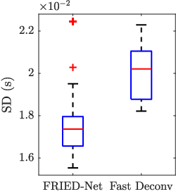
To quantitatively compare our approach against the broadly used probabilistic fast deconvolution algorithm [49], we present the receiver operating characteristic (ROC) curves of the respective techniques in Fig. 17(b). It is plotted by changing the threshold of the probability histogram between 0 and 1 to illustrate the trade-off between the spike detection rate and the false positive rate. Here, the acceptance interval is chosen to be double the sampling period, that is s. We observe that FRIED-Net performs competitively over the fast deconvolution algorithm, as it achieves a true positive rate of . We further compare the precision of the true positives. Again, we use the standard deviation described in (18) as the evaluation metric. Fig. 17(c) presents the distribution of standard deviation of the detected locations with respect to the ground truth locations with changing probability threshold, where outliers are indicated by the red crosses. We see that the overall standard deviation of FRIED-Net is lower than that of the fast deconvolution algorithm. This shows that our approach provides more precise estimations.
VI Conclusion
This paper addresses limitations of existing FRI techniques in that the reconstruction performance breaks down in the presence of noise caused by the so-called subspace swap event. We proposed two learning-based FRI reconstruction algorithms that are inspired by the classical FRI reconstruction models. Deep Unfolded PWGD provides an interpretable deep neural network based on existing iterative denoising algorithm for subspace-based methods, while FRIED-Net aims to bypass subspace-based algorithms and instead models the acquisition process of FRI signals. The latter is particularly useful in neuroscience applications where the sampling kernel is unknown, since it can be learned using backpropagation. Simulation results show that despite a slight compromise at high PSNR, our proposed approaches reconstruct FRI signals in the low PSNR region where existing FRI algorithms break down, even when the original sampling kernel is unknown. We then demonstrated that our proposed approach provides more precise spike detection than existing algorithms on real-life calcium imaging data, while maintaining a similar performance in terms of true positive and false positive rate.
References
- [1] Y. C. Eldar, Sampling Theory: Beyond Bandlimited Systems. Cambridge University Press, 2014.
- [2] M. Vetterli, P. Marziliano, and T. Blu, “Sampling signals with finite rate of innovation,” IEEE Transactions on Signal Processing, vol. 50, no. 6, pp. 1417–1428, Jun. 2002.
- [3] P. L. Dragotti, M. Vetterli, and T. Blu, “Sampling moments and reconstructing signals of finite rate of innovation: Shannon meets Strang-Fix,” IEEE Transactions on Signal Processing, vol. 55, no. 5 I, pp. 1741–1757, 2007.
- [4] T. Blu, P. L. Dragotti, M. Vetterli, P. Marziliano, and L. Coulot, “Sparse sampling of signal innovations: Theory, algorithms, and performance bounds,” IEEE Signal Processing Magazine, vol. 25, no. 2, pp. 31–40, 2008.
- [5] J. A. Urigüen, T. Blu, and P. L. Dragotti, “FRI sampling with arbitrary kernels,” IEEE Transactions on Signal Processing, vol. 61, no. 21, pp. 5310–5323, 2013.
- [6] R. Tur, Y. C. Eldar, and Z. Friedman, “Innovation rate sampling of pulse streams with application to ultrasound imaging,” IEEE Transactions on Signal Processing, vol. 59, no. 4, pp. 1827–1842, 2011.
- [7] J. Oñativia, S. R. Schultz, and P. L. Dragotti, “A finite rate of innovation algorithm for fast and accurate spike detection from two-photon calcium imaging,” Journal of Neural Engineering, vol. 10, no. 4, pp. 46 017–46 031, 2013.
- [8] Z. Doğan, T. Blu, and D. Van De Ville, “Detecting spontaneous brain activity in functional magnetic resonance imaging using finite rate of innovation,” in 2014 IEEE International Symposium on Biomedical Imaging (ISBI), Jul. 2014, pp. 1047–1050.
- [9] O. Bar-Ilan and Y. C. Eldar, “Sub-Nyquist radar via doppler focusing,” IEEE Transactions on Signal Processing, vol. 62, no. 7, pp. 1796–1811, 2014.
- [10] N. Wagner, Y. C. Eldar, and Z. Friedman, “Compressed beamforming in ultrasound imaging,” IEEE Transactions on Signal Processing, vol. 60, no. 9, pp. 4643–4657, 2012.
- [11] Y. Hao, P. Marziliano, M. Vetterli, and T. Blu, “Compression of ECG as a signal with finite rate of innovation,” in Annual International Conference of the IEEE Engineering in Medicine and Biology, vol. 7, 2005, pp. 7564–7567.
- [12] R. Prony, “Essai expérimental et analytique sur les lois de la dilatabilité des fluides élastiques, et sur celles de la force expansive de la vapeur de l’eau et de la vapeur de l’alkool, á différentes temperatures,” J. de l’Ecole Polytechnique, vol. 1, pp. 24–76, 1795.
- [13] J. A. Cadzow, “Signal enhancement - A composite property mapping algorithm,” IEEE Transactions on Acoustics, Speech, and Signal Processing, vol. 36, no. 1, pp. 49–62, 1988.
- [14] Y. Hua and T. K. Sarkar, “Matrix pencil method for estimating parameters of exponentially damped/undamped sinusoids in noise,” IEEE Transactions on Acoustics, Speech, and Signal Processing, vol. 38, no. 5, pp. 814–824, May 1990.
- [15] H. Cramér, Mathematical Methods of Statistics. Princeton university press, 1946.
- [16] C. R. Rao, “Information and the accuracy attainable in the estimation of statistical parameters,” Bulletin of Calcutta Mathematical Society, vol. 37, pp. 81–89, 1945.
- [17] X. Wei and P. L. Dragotti, “Guaranteed performance in the FRI setting,” IEEE Signal Processing Letters, vol. 22, no. 10, pp. 1661–1665, 2015.
- [18] J. K. Thomas, L. L. Scharf, and D. W. Tufts, “The probability of a subspace swap in the SVD,” IEEE Transactions on Signal Processing, vol. 43, no. 3, pp. 730–736, 1995.
- [19] B. N. Bhaskar, G. Tang, and B. Recht, “Atomic norm denoising with applications to line spectral estimation,” IEEE Transactions on Signal Processing, vol. 61, no. 23, pp. 5987–5999, 2013.
- [20] G. Tang, B. N. Bhaskar, P. Shah, and B. Recht, “Compressed sensing off the grid,” IEEE Transactions on Information Theory, vol. 59, no. 11, pp. 7465–7490, 2013.
- [21] E. J. Candès and C. Fernandez-Granda, “Towards a mathematical theory of super-resolution,” Communications on Pure and Applied Mathematics, vol. 67, no. 6, pp. 906–956, 2014.
- [22] S. Mulleti, K. Lee, and Y. C. Eldar, “Identifiability conditions for compressive multichannel blind deconvolution,” IEEE Transactions on Signal Processing, vol. 68, pp. 4627–4642, 2020.
- [23] B. Tolooshams, S. Mulleti, D. Ba, and Y. C. Eldar, “Learning filter-based compressed blind-deconvolution,” arXiv:2209.14165, Sep. 2022.
- [24] G. Mathew and V. U. Reddy, “Development and analysis of a neural network approach to pisarenko’s harmonic retrieval method,” IEEE Transactions on Signal Processing, vol. 42, no. 3, pp. 663–667, 1994.
- [25] G. Izacard, S. Mohan, and C. Fernandez-Granda, “Data-driven estimation of sinusoid frequencies,” in Advances in Neural Information Processing Systems, vol. 32, 2019, pp. 5127–5137.
- [26] G. Izacard, B. Bernstein, and C. Fernandez-Granda, “A learning-based framework for line-spectra super-resolution,” in 2019 IEEE International Conference on Acoustics, Speech and Signal Processing (ICASSP). IEEE, May 2019, pp. 3632–3636.
- [27] S. Adavanne, A. Politis, and T. Virtanen, “Direction of arrival estimation for multiple sound sources using convolutional recurrent neural network,” in 2018 European Signal Processing Conference (EUSIPCO), Nov. 2018, pp. 1462–1466.
- [28] X. Xiao et al., “A learning-based approach to direction of arrival estimation in noisy and reverberant environments,” in 2015 IEEE International Conference on Acoustics, Speech and Signal Processing (ICASSP), 2015, pp. 2814–2818.
- [29] N. Shlezinger, J. Whang, Y. C. Eldar, and A. G. Dimakis, “Model-based deep learning: Key approaches and design guidelines,” in 2021 IEEE Data Science and Learning Workshop, DSLW 2021, Jun. 2021.
- [30] K. Gregor and Y. LeCun, “Learning fast approximations of sparse coding,” in 2010 International Conference on Machine Learning (ICML), 2010, pp. 399–406.
- [31] V. Monga, Y. Li, and Y. C. Eldar, “Algorithm unrolling: Interpretable, efficient deep learning for signal and image processing,” IEEE Signal Processing Magazine, vol. 38, no. March, pp. 18–44, 2021.
- [32] O. Solomon et al., “Deep unfolded robust PCA with application to clutter suppression in ultrasound,” IEEE Transactions on Medical Imaging, vol. 39, no. 4, pp. 1051–1063, 2020.
- [33] J.-F. Cai, S. Liu, and W. Xu, “A fast algorithm for reconstruction of spectrally sparse signals in super-resolution,” in Wavelets and Sparsity XVI, vol. 9597. SPIE, Aug. 2015, p. 95970A.
- [34] Z. Dang et al., “Eigendecomposition-free training of deep networks with zero eigenvalue-based losses,” in 2018 European Conference on Computer Vision (ECCV), 2018, pp. 768–783.
- [35] V. C. H. Leung, J.-J. Huang, Y. C. Eldar, and P. L. Dragotti, “Reconstruction of FRI signals using autoencoders with fixed decoders,” in 2021 European Signal Processing Conference (EUSIPCO), 2021, pp. 1496–1500.
- [36] M. Unser and T. Blu, “Cardinal exponential splines: Part I - theory and filtering algorithms,” IEEE Transactions on Signal Processing, vol. 53, no. 4, pp. 1425–1438, 2005.
- [37] I. Markovsky, “Structured low-rank approximation and its applications,” Automatica, vol. 44, no. 4, pp. 891–909, Apr. 2008.
- [38] M. Fazel, H. Hindi, and S. P. Boyd, “A rank minimization heuristic with application to minimum order system approximation,” in 2001 American Control Conference (ACC), vol. 6, 2001, pp. 4734–4739.
- [39] L. Condat and A. Hirabayashi, “Cadzow denoising upgraded: A new projection method for the recovery of dirac pulses from noisy linear measurements,” Sampling Theory in Signal and Image Processing, vol. 14, no. 1, pp. 17–47, 2015.
- [40] D. P. Kingma and J. Ba, “Adam: A Method for Stochastic Optimization,” in 2015 International Conference on Learning Representations (ICLR), San Diego, CA, USA, 2015.
- [41] V. C. H. Leung, J.-J. Huang, and P. L. Dragotti, “Reconstruction of FRI signals using deep neural network approaches,” in 2020 IEEE International Conference on Acoustics, Speech and Signal Processing (ICASSP), 2020, pp. 5430–5434.
- [42] K. Hornik, M. Stinchcombe, and H. White, “Multilayer feedforward networks are universal approximators,” Neural Networks, vol. 2, no. 5, pp. 359–366, 1989.
- [43] M. Leshno, V. Y. Lin, A. Pinkus, and S. Schocken, “Multilayer feedforward networks with a nonpolynomial activation function can approximate any function,” Neural Networks, vol. 6, no. 6, pp. 861–867, 1993.
- [44] U. Shaham, A. Cloninger, and R. R. Coifman, “Provable approximation properties for deep neural networks,” Applied and Computational Harmonic Analysis, vol. 44, no. 3, pp. 759–773, Sep. 2018.
- [45] A. Paszke et al., “PyTorch: An imperative style, high-performance deep learning library,” in Advances in Neural Information Processing Systems, vol. 32. Curran Associates, Inc., 2019, pp. 8024–8035.
- [46] R. Yasuda et al., “Imaging calcium concentration dynamics in small neuronal compartments.” Science’s STKE : signal transduction knowledge environment, vol. 2004, no. 219, 2004.
- [47] T. W. Chen et al., “Ultrasensitive fluorescent proteins for imaging neuronal activity,” Nature, vol. 499, no. 7458, pp. 295–300, 2013.
- [48] K. Svoboda, “Simultaneous imaging and loose-seal cell-attached electrical recordings from neurons expressing a variety of genetically encoded calcium indicators,” GENIE Project, Janelia Farm Campus, 2015, CRCNS.org.
- [49] J. T. Vogelstein et al., “Fast nonnegative deconvolution for spike train inference from population calcium imaging,” Journal of Neurophysiology, vol. 104, no. 6, pp. 3691–3704, Dec. 2010.