Large baseline optical imaging assisted by single photons and linear quantum optics
Abstract
In this work, we show that by combining quantum metrology and networking tools, it is possible to extend the baseline of an interferometric optical telescope and thus improve diffraction-limited imaging of point source positions. The quantum interferometer is based on single-photon sources, linear optical circuits, and efficient photon number counters. Surprisingly, with thermal (stellar) sources of low photon number per mode and high transmission losses across the baseline, the detected photon probability distribution still retains a large amount of Fisher information about the source position, allowing for a significant improvement in the resolution of positioning point sources, on the order of 10 as. Our proposal can be implemented with current technology. In particular, our proposal does not require experimental optical quantum memories.
Telescopes can be improved in several ways: improving the signal-to-noise ratio Pearce et al. 2017; Howard et al. 2019, employing (quantum) designs to achieve super-resolution Kolobov 2007; Tsang et al. 2016; Paúr et al. 2016; Tsang 2019; Lupo et al. 2020; Zanforlin et al. 2022; Brown et al. 2022a, or extending the baseline to create larger apertures Dravins 2016; Akiyama et al. 2019; Bojer et al. 2020; Czupryniak et al. 2021; Brown et al. 2022b. The resolving power of an optical imaging system can be defined in terms of the minimum resolvable angle , which depends on the source’s wavelength and on the telescope’s aperture size. Larger aperture sizes give better resolving power. In astronomy, large baseline interferometric telescopes have become an established technique to create highly resolved images. One of the most notable results achieved with this technique is the first-ever radio image of a black hole Akiyama et al. 2019, produced by a combination of many telescopes that formed a single imaging system with an aperture the size of the Earth. The receivers measured the phase and amplitude of the radio signals, and combined them into an interferometric image.
For optical signals, the frequency is too high to measure the phase and amplitude of the incoming light directly, and the incoming signals must be made to interfere physically. This places a limit on how far receivers can be placed apart, since the transmission of the signal in optical fibres or light tunnels is lossy Townsend et al. 1993. A solution involving teleporting photons from the receiver to the interferometric setup demonstrates how quantum information technology can overcome this limitation using optical quantum memories Gottesman et al. 2012; Khabiboulline et al. 2019. Recently, a large-baseline quantum telescope was proposed that makes use of photonic quantum memories and error correction to protect the weak optical signal from transmission losses Huang et al. 2022.
While future quantum technologies can deliver major improvements to large baseline optical telescopes, near-future telescopes must rely on more readily available technologies. Here, we propose a large-baseline optical telescope that employs single photon sources Kaneda and Kwiat 2019; Kennard et al. 2013; Fulconis et al. 2005; Silverstone et al. 2014, low-loss optical fibres, linear optical interferometry Wang et al. 2020; Carolan et al. 2015, and high-efficiency photon number counters McMillan et al. 2013; Paesani et al. 2020. Our proposal uses multiple single-photon sources and optical quantum Fourier transform (QFT) circuits, shown in Fig. 1, which is a linear optical circuit where a photon entering any input mode is equally likely to to appear in any output mode. Here, we demonstrate that establishing coherence across the baseline using multiple single photon sources and beam splitters improves the resolution of the telescope, even when the transmission losses along the baseline are high.
Our setup is as follows: a simple interferometric telescope employs two receivers, A and B, a distance apart. A distant star-source emits incoherent light that can be described as a single mode with large transverse coherence reaching the telescope at an angle . At any given optical frequency, the distant star emits a weak incoherent signal such that we can assume at most single photon events with probability . The state of a single photon entering the two receivers is given by
| (1) |
where and indicates the zero and one photon state at each receiver, and is the relative phase shift between the two receivers. It arises from the additional distance in the light-path at one of the receivers, and , where is the wave number of the source. For distant star-sources a very good approximation is . The quantum Fisher information for in the state is 1 (see Supplementary Material).
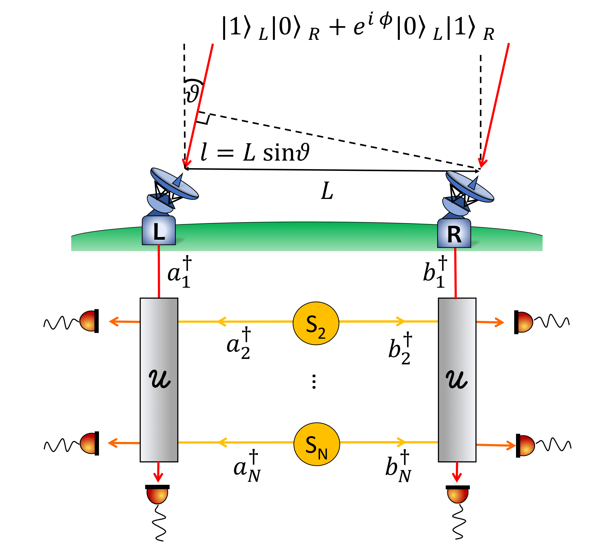
In an ideal scenario there is no loss, and the interferometric measurement can be simply performed by recombining the photon through a beam-splitter. However, a major challenge is the physical transportation of the photon from one site to the other. In a realistic dissipative scenario the photon loss thus limits the baseline . In our proposal, the star photon () does not travel a large distance from the receiver, and incurs minimal loss. Instead, single photons generated in ground-based sources () are sent to the two receivers, and , in the single-photon Bell state
| (2) |
which can be produced using a 50:50 beam splitter. At each receiver, we let these photons interfere with the optical mode from the starlight in a QFT circuit, and the output modes are measured in highly efficient photon counting detectors Hadfield 2009; Esmaeil Zadeh et al. 2021; Natarajan et al. 2012; Hadfield et al. 2006; Miller et al. 2003. The information of the signal we intend to measure is contained in the correlations between the detectors at the receivers. By using multiple ground-based photon sources, we aim to overcome the large transmission losses between the receivers.
We treat the imaging protocol above as a quantum parameter estimation problem for Paris 2009; Giovannetti et al. 2006; Giovannetti et al. 2011; Demkowicz-Dobrzanski et al. 2009; Knott et al. 2016, which is directly related to . The ultimate precision with which it is possible to measure is given by the Cramér-Rao bound Helstrom 1976, which represents a lower bound to the variance of an estimator of , given the knowledge of the quantum mechanical state . For unbiased estimators, the bound is given by the inverse of the Fisher information associated with the state
| (3) |
where is the number of independent measurements. The Fisher information
| (4) |
is given in terms of the probabilities of measuring the outcome when the parameter has fixed value .
First, we consider a single ground-based photon and a single star photon. If both photons are detected by the same receiver, then is at most a global phase in the quantum state, and the measurements will not reveal any information about . Only when the two photons are detected at different receivers do we gain information about . This limits the Fisher information to . To increase the Fisher information, we can increase the number of ground-based photons to , which means that the probability of measuring all photons at the same receiver becomes , and the resulting Fisher information is bounded by
| (5) |
At this point, we have assumed no losses in the transmission, and we did not make assumptions about the precise interferometer at both receivers.
Next, we introduce the model for describing the quantum telescope with ground-based photons. We will describe the lossless case first. The total initial state is
| (6) |
where the first photon comes from the star-source and its initial state is given by Eq. (1), and the other photons are in the state , given in Eq. (2). In terms of creation and annihilation operators and for each photon mode, the state becomes
| (7) |
where is the Kronecher delta indicating that the relative phase shift enters just in the mode of the star-source , and is the vacuum state for all the modes. For the interferometry between the star-photon and the lab-photons we choose a linear transformation that implements a QFT Reck et al. 1994. For each of the input modes on the right
| (8) |
and analogously for the input modes on the left. The output state is then
| (9) |
The probability of measuring a given configuration of photons across the detectors is
| (10) |
where is the measured state with photons at the detector . We recast the Fisher information in terms of these probabilities, as
| (11) |
where the sum runs over all the possible configurations of photons distributed across detectors. For the lossless case, is shown in the Supplementary Material (see Fig. 5).
The ground-based photons are subject to transmission losses, which can be modelled using a beam splitter in the transmission line. This is shown in Fig. 2. The transmission probability amplitude of a photon in an optical fibre is given by , where we use that each photon travels over a length , and is the fibre attenuation length—assumed identical for all transmission lines. The transformation for the -photon mode operators is thus
| (12) |
where and are the creation and annihilation operators for the vacuum fields respectively on the left and right side.

For now, we consider the presence of exactly one star-photon. The state of the optical modes in Eq. (7) at the QFT circuits in the presence of loss becomes
| (13) |
where is the probability of losing a single photon.
The number of detected photons is no longer equal to ; it runs in the interval . The Fisher information will be modified, since it will include the probabilities for partial photon detection. In the Supplementary Material we show that this can be rewritten as the weighted sum of Fisher information contributions corresponding to partial photon detection
| (14) |
where is the Fisher information for photon detected, is the number of photons lost.
Next, we consider the case where the starlight is in a thermal state at an optical frequency with a rate of photon emission much smaller than 1 Mandel and Wolf 1995. Therefore, the density operator for the initial state of the star light can be well approximated as , where is the one-photon state from Eq. (6), and is the zero-photon state. The probability of detecting photons is given by the sum of two probabilities as
| (15) |
where and are the probability distributions for having no star photon and having a star photon, respectively. This means that when detecting photons, there will be two contributions to the total probability distribution, arising from the fact that we can not distinguish whether the reduced photon number is due to lossy transmission of the ground-based photons or an absence of the star photon.
The Fisher information must be modified as follows (see Supplementary Materials)
| (16) |
and by using Eq. (15) we obtain
| (17) |
Here, we used that in the absence of a star photon the probability distribution does not depend on , and the contribution to the derivative is zero. We calculated the Fisher information for the cases , but these expressions are too large to include here.
The total Fisher information is modified by the factor, which is usually very small. A Fisher information scaling linearly in reflects the reduced rate of gaining information about . However, when scales with , this would indicate that the transmission losses obscure the absence of a star photon, leading to a much deteriorated metrology protocol and a very large estimation error. Surprisingly, we find that for the cases we examined (), the Fisher information scales linearly in , as shown in Fig. 3. This can be understood by considering that the transmission loss and the absence of a star photon occur in orthogonal optical modes, rendering and quite different. Consequently, our protocol is still able to provide an improvement in the resolution of (and therefore ).
Finally, we study the resolution of the telescope in terms of the error in the geometrical angle under the small angle approximation. The mean square error is given by
| (18) |
where is the variance associated with the relative phase shift, lower bounded by the Fisher information. Therefore, the minimum error on the resolution is given by
| (19) |
The resolution will be better for higher values of the Fisher information and for large distances between the telescopes, in accordance with the Rayleigh criterion.
The resolution of the telescope will improve when we increase the distance between the receivers, but increased transmission photon loss will deteriorate the resolution. Therefore, we must find the optimal distance between receivers for photon-assisted interferometric imaging. This is shown in Fig. 4. For light with a wavelength nm and fibre attenuation length km, an angular resolution of as (micro arcseconds) is achievable with a single ground-based photon (), while four ground-based photons () yields an angular resolution of as. For increasing , the best resolution is obtained for larger distances, indicating that the extra ground-based photons help increase the baseline, and hence the resolution. We summarise the optimal distances and the achievable resolution in Table 1. Moreover, the corresponding optimal relative phase shift is determined by the orientation of the baseline, and can be set by including an adjustable phase shift at one of the receivers.
| () | (rad) | ||
|---|---|---|---|
| 2 | 19.80 | 3.99 | 0.318 |
| 3 | 15.52 | 4.17 | 0.724 |
| 4 | 12.26 | 4.56 | 0.513 |
| 5 | 10.93 | 4.79 | 0.247 |
Conclusions- We addressed the challenge of increasing the resolution of positioning incoherent point sources in interferometric telescopes at optical frequencies by extending the baseline of the telescope. We showed that a dramatic imaging resolution improvement can be obtained with a setup that relies solely on current technology (multiple single-photon sources, optical fibres, linear optical circuits and photon number counting detectors), without the need for quantum memories or full-scale quantum repeater networks. This is an example of a useful near- to medium-term quantum technology application beyond quantum key distribution.
Transmitting multiple single photons across the baseline with high transmission losses extends the numerical aperture to tens of kilometres for optical frequencies, leading to a resolution on the order of 10 as. One may expect that losing photons in an interferometric measurement will drastically reduce the Fisher information, since we cannot distinguish between photons that are lost in transmission or that were not emitted by the source in the first place. However, the Fisher information scales linearly rather than quadratic in , which accounts for this unexpected good performance. Our results are important for our theoretical understanding of optical interferometers in metrology applications, since they point towards a pathway for loss-tolerant optical quantum metrology where signal photons and auxiliary optical states interfere. It may help extend the range of optical communication without full quantum repeaters.
Finally, our analysis is not limited to ground-based telescopes and apply equally to satellite-based receivers where the single photon sources are distributed through free space. The beam divergence is the main loss mechanism, leading to much larger baselines on the order of 1 000 km or a resolution of 50 nas.
Acknowledgements. We thank Zixin Huang, Cosmo Lupo, and Francesco Albarelli for valuable discussions and suggestions. This work is funded by the EPSRC Large Baseline Quantum-Enhanced Imaging Networks Grant No. EP/V021303/1, and the EPSRC Quantum Communications Hub, Grant No. EP/M013472/1.
References
- Pearce et al. (2017) M. E. Pearce, E. T. Campbell, and P. Kok, Quantum 1, 21 (2017).
- Howard et al. (2019) L. A. Howard, G. G. Gillett, M. E. Pearce, R. A. Abrahao, T. J. Weinhold, P. Kok, and A. G. White, Phys. Rev. Lett. 123, 143604 (2019).
- Kolobov (2007) M. Kolobov, Quantum Imaging (Springer New York, 2007).
- Tsang et al. (2016) M. Tsang, R. Nair, and X.-M. Lu, Physical Review X 6, 031033 (2016).
- Paúr et al. (2016) M. Paúr, B. Stoklasa, Z. Hradil, L. L. Sánchez-Soto, and J. Rehacek, Optica 3, 1144 (2016).
- Tsang (2019) M. Tsang, Contemporary Physics 60, 279 (2019).
- Lupo et al. (2020) C. Lupo, Z. Huang, and P. Kok, Phys. Rev. Lett. 124, 080503 (2020).
- Zanforlin et al. (2022) U. Zanforlin, C. Lupo, P. W. R. Connolly, P. Kok, G. S. Buller, and Z. Huang, Nature Comms. 13, 5373 (2022).
- Brown et al. (2022a) M. R. Brown, M. Allgaier, V. Thiel, J. Monnier, M. G. Raymer, and B. J. Smith, arXiv:2212.07395 (2022a).
- Dravins (2016) D. Dravins, Proc. SPIE, Optical and Infrared Interferometry and Imaging V 9907, 0M (2016).
- Akiyama et al. (2019) K. Akiyama, A. Alberdi, W. Alef, K. Asada, R. Azulay, A.-K. Baczko, D. Ball, M. Baloković, J. Barrett, D. Bintley, et al., The Astrophysical Journal Letters 875, L4 (2019).
- Bojer et al. (2020) M. Bojer, Z. Huang, S. Karl, S. Richter, P. Kok, and J. von Zanthier, New J. Phys. 24, 043026 (2020).
- Czupryniak et al. (2021) R. Czupryniak, J. Steinmetz, P. G. Kwiat, and A. N. Jordan, arXiv:2108.01170 (2021), https://doi.org/10.48550/arXiv.2108.01170.
- Brown et al. (2022b) M. R. Brown, M. Allgaier, V. Thiel, J. Monnier, M. G. Raymer, , and B. J. Smith, arXiv:2212.07395 (2022b), https://doi.org/10.48550/arXiv.2212.07395.
- Townsend et al. (1993) P. D. Townsend, J. Rarity, and P. Tapster, Electronics Letters 7, 634 (1993).
- Gottesman et al. (2012) D. Gottesman, T. Jennewein, and S. Croke, Physical review letters 109, 070503 (2012).
- Khabiboulline et al. (2019) E. T. Khabiboulline, J. Borregaard, K. De Greve, and M. D. Lukin, Physical review letters 123, 070504 (2019).
- Huang et al. (2022) Z. Huang, G. K. Brennen, and Y. Ouyang, Phys. Rev. Lett. 129, 210502 (2022).
- Kaneda and Kwiat (2019) F. Kaneda and P. G. Kwiat, Science advances 5, eaaw8586 (2019).
- Kennard et al. (2013) J. Kennard, J. Hadden, L. Marseglia, I. Aharonovich, S. Castelletto, B. Patton, A. Politi, J. Matthews, A. Sinclair, B. Gibson, et al., Physical review letters 111, 213603 (2013).
- Fulconis et al. (2005) J. Fulconis, O. Alibart, W. Wadsworth, P. S. J. Russell, and J. Rarity, Optics Express 13, 7572 (2005).
- Silverstone et al. (2014) J. W. Silverstone, D. Bonneau, K. Ohira, N. Suzuki, H. Yoshida, N. Iizuka, M. Ezaki, C. M. Natarajan, M. G. Tanner, R. H. Hadfield, et al., Nature Photonics 8, 104 (2014).
- Wang et al. (2020) J. Wang, F. Sciarrino, A. Laing, and M. G. Thompson, Nature Photonics 14, 273 (2020).
- Carolan et al. (2015) J. Carolan, C. Harrold, C. Sparrow, E. Martín-López, N. J. Russell, J. W. Silverstone, P. J. Shadbolt, N. Matsuda, M. Oguma, M. Itoh, et al., Science 349, 711 (2015).
- McMillan et al. (2013) A. McMillan, B. Bell, A. Clark, L. Labonté, S. Kannan, W. McCutcheon, T. Wu, A. Martin, O. Alibart, S. Tanzilli, et al., in Laser Science (Optica Publishing Group, 2013) pp. LTu4G–3.
- Paesani et al. (2020) S. Paesani, M. Borghi, S. Signorini, A. Maïnos, L. Pavesi, and A. Laing, Nature communications 11, 1 (2020).
- Hadfield (2009) R. H. Hadfield, Nature photonics 3, 696 (2009).
- Esmaeil Zadeh et al. (2021) I. Esmaeil Zadeh, J. Chang, J. W. Los, S. Gyger, A. W. Elshaari, S. Steinhauer, S. N. Dorenbos, and V. Zwiller, Applied Physics Letters 118, 190502 (2021).
- Natarajan et al. (2012) C. M. Natarajan, M. G. Tanner, and R. H. Hadfield, Superconductor science and technology 25, 063001 (2012).
- Hadfield et al. (2006) R. H. Hadfield, J. L. Habif, J. Schlafer, R. E. Schwall, and S. W. Nam, Applied physics letters 89, 241129 (2006).
- Miller et al. (2003) A. J. Miller, S. W. Nam, J. M. Martinis, A. V. Sergienko, et al., (2003).
- Paris (2009) M. G. Paris, International Journal of Quantum Information 7, 125 (2009).
- Giovannetti et al. (2006) V. Giovannetti, S. Lloyd, and L. Maccone, Physical review letters 96, 010401 (2006).
- Giovannetti et al. (2011) V. Giovannetti, S. Lloyd, and L. Maccone, Nature photonics 5, 222 (2011).
- Demkowicz-Dobrzanski et al. (2009) R. Demkowicz-Dobrzanski, U. Dorner, B. Smith, J. Lundeen, W. Wasilewski, K. Banaszek, and I. Walmsley, Physical Review A 80, 013825 (2009).
- Knott et al. (2016) P. A. Knott, T. J. Proctor, A. J. Hayes, J. F. Ralph, P. Kok, and J. A. Dunningham, Physical Review A 94, 062312 (2016).
- Helstrom (1976) C. Helstrom, Quantum Detection and Estimation Theory, Vol. 84 (New York: Academic, 1976).
- Reck et al. (1994) M. Reck, A. Zeilinger, H. J. Bernstein, and P. Bertani, Physical review letters 73, 58 (1994).
- Mandel and Wolf (1995) L. Mandel and E. Wolf, Optical coherence and quantum optics (Cambridge university press, 1995).
Appendix A Quantum Fisher information for a single phase
We show here that the Quantum Fisher information of for the state is equal to one. The Quantum Fisher information
| (20) |
is expressed in terms of the variance associated with the generator . Therefore, we can directly compute the variance on the state as
| (21) |
It follows that the Quantum Fisher information is .
Appendix B From the -photon to -photon case
We discuss in detail the simplest scenario consisting of only two photon sources, one for the star photon, and the other for the ground-based photon. The total initial state is the tensor product of the star photon state, given by Eq. (1), and the ground-based photon state, from Eq. (2),
| (22) |
where we simplified the notation by omitting the subscripts .
It is convenient to rewrite the initial state in term of the creation/annihilation operators, as
| (23) |
where we called () the operators for the right (left) states, and the index indicates either the star source or the ground-based photon source ; is the total vacuum state.
At each site, the star photon modes are mixed with the ground-based photon modes according to the linear QFT evolution from Eq. (8). For the case this transformation takes the form of a simple 50:50 beam-splitter, that gives the following outputs for the modes on the right
| (24) |
and analogously for the modes on the left. Therefore, the initial state in Eq. (23) will be transformed into the final state
| (25) |
To compute the Fisher information we need the probabilities
| (26) |
for all the configurations , where is the number of detected photons. By looking at the probabilities, for this simple case, there are ten possible ways of distributing 2 photons among the four detectors. However, only when the 2 photons are detected on different sides we can extract information on . This happens for four configurations, that will give probabilities
| (27) |
All the other configurations will give probabilities that do not depend on . In fact, when both photons are detected by the same detector or by different detectors on the same side, the relative phase shift will be just a global phase. The majority of cases will not bring any contribution to the Fisher information. The Fisher information from Eq. (4), in the 2-photon case, results to be constant
| (28) |
The generalization to -photons scenario, where the set-up is endowed with ground-based photon sources, increases the number of probabilities of detecting photons on both sides. This will result into more contributions to the Fisher information and smaller variance. The plots in Fig. 5 show the Fisher information in function of the relative phase shift for different number of photons. As expected, in the ideal no-loss case scenario, the larger number of photons results in a higher Fisher information. For small angles, the Fisher information is approximately constant and it scales with as . In the ideal scenario, with no loss, increasing results in higher values of the Fisher information and lower variances associated to the phase shift angle .
Appendix C Additivity of Fisher information
We derive an expression for the Fisher information for photons when the ground-based photons are subjected to transmission losses. This results in a sum of contributions corresponding to the Fisher information of partial photon detection.
Consider the case of 1 star photon and ground-based photons in presence of loss. We assume for now that the star photon is not subjected to any loss. We call the number of lost photons and the number of detected photons. Let’s call the set of all the configurations we obtain from measuring photons. Thus, there will be cases corresponding to losses of different number of photons, i.e., . The two extreme cases are , the set of configurations corresponding to the no-loss scenario, or equivalently all the photons are detected; and the set of configurations for the case in which all the ground-based photons are lost and only the star photon is detected.
For a given number of detected photon, will contain configurations; each configuration has a probability
| (29) |
The Fisher information from Eq. (11) has to be the sum of all the probabilities, thus
| (30) |
where the sum over runs over all the possible configurations for detected photons, and the other sum accounts for all the possible values of . The set of probabilities for a given number of detected photons is not normalized, meaning that the sum does not add up to one, but to a certain value that corresponds to the total probability of detecting photons
| (31) |
Therefore we rewrite these probabilities in terms of a new set of normalized probabilities
| (32) |
We can use this expression for the Fisher information of Eq. (30) and, by using the logarithmic properties and the fact that the coefficients do not depend on , we obtain
| (33) |
Now we can recognize that this is a sum of Fisher information for different values of weighted with the factor
| (34) |
where we called
| (35) |
Note that these contributions do not correspond to the Fisher information from Eq. (11) with a different number of photons. They are computed by using the probabilities of distributing photons in detectors, therefore only the first term , optimal detection case, coincide with Eq. (5). The value is the probability of detecting photons, and it is given by
| (36) |
where is the probability of losing one photon and the binomial factor arises from the fact that the lost photons are not distinguishable. We point out that is always zero because in the presence of only one detected photon, , we have no information about the correlations. By substituting in Eq. (34) we recover the expression from Eq. (14). In Fig. 6 we present the Fisher information when the photon loss is included. We compare the situations with , , ground-based photons, and we notice that increasing results in a lower value of the Fisher information.
Appendix D Fisher information for lossy case
The Fisher information in the no-loss case is given by Eq. (11), where the probabilities are of the detector signatures . In the lossy case, we still have a probability distribution over the detector signatures , but the total photon count is no longer always , so generally can be written as
| (37) |
where is the outcome set of detected photons. By using the chain rule, we obtain Eq. (16).