Evidence for the volatile-rich composition of a 1.5- planet
Abstract
The population of planets smaller than approximately is widely interpreted as consisting of rocky worlds, generally referred to as super-Earths. This picture is largely corroborated by radial-velocity (RV) mass measurements for close-in super-Earths but lacks constraints at lower insolations. Here we present the results of a detailed study of the Kepler-138 system using 13 Hubble and Spitzer transit observations of the warm-temperate planet Kepler-138 d () combined with new Keck/HIRES RV measurements of its host star. We find evidence for a volatile-rich “water world” nature of Kepler-138 d, with a large fraction of its mass contained in a thick volatile layer. This finding is independently supported by transit timing variations, RV observations (), as well as the flat optical/IR transmission spectrum. Quantitatively, we infer a composition of % volatiles by mass or by volume, with a 2000 km deep water mantle and atmosphere on top of a core with an Earth-like silicates/iron ratio. Any hypothetical hydrogen layer consistent with the observations () would have swiftly been lost on a Myr timescale. The bulk composition of Kepler-138 d therefore resembles those of the icy moons rather than the terrestrial planets in the solar system. We conclude that not all super-Earth-sized planets are rocky worlds, but that volatile-rich water worlds exist in an overlapping size regime, especially at lower insolations. Finally, our photodynamical analysis also reveals that Kepler-138 c (, ) is a slightly warmer twin of Kepler-138 d, i.e., another water world in the same system, and we infer the presence of Kepler-138 e, a likely non-transiting planet at the inner edge of the habitable zone.
We observed 13 new transits of Kepler-138 d with HST and Spitzer (Table 1) as part of the HST survey program GO 13665 (PI Benneke, three transits) and the Spitzer program GO 11131 (PI Dragomir, five transits at 3.6 m and five transits at 4.5 m). We chose the Kepler-138 system for this detailed study because the three known transiting planets on near-resonant orbits open a rare opportunity for measuring the masses of low-temperature, super-Earth-sized planets 1; 2; 3; 4. The HST and Spitzer observations critically extend the baseline for the transit-timing variations (TTV) analysis to over 7 years. Therefore, the new transits enable our analysis to cover nearly two super-periods of TTV modulation for the interaction of Kepler-138 c and d, almost doubling the baseline compared to the Kepler transit timing measurements alone. We complement this dataset with 28 Keck/HIRES RV measurements of Kepler-138 that support the TTV analysis. The HST/WFC3 and Spitzer/IRAC light curves are extracted using the ExoTEP pipeline. The transit parameters are then constrained for each visit by jointly fitting a set of astrophysical and instrumental model parameters (see Methods). We ensure the robustness of our transit analyses by verifying the statistical consistency of transit depths from individual visits with the same instrument. We also find that the transit timing constraints are consistent for a transit simultaneously observed with HST and Spitzer (Table 1).
Results Our measured HST and Spitzer transit times for Kepler-138 d (Table 1) are inconsistent with the forward predictions from the photodynamical fit to the Kepler transits (Supplementary Figure 1). We therefore revisit the orbital solution using an MCMC analysis of the transit-timing variations (TTV) over the full 7-year dataset combining Kepler, HST and Spitzer transits (see Methods). No three-planet model can simultaneously reproduce the Kepler, HST, and Spitzer transit times of Kepler-138 d (Figure 1abc, Extended Data Figure 1). We therefore explore possible orbits and masses of a fourth planet (see Methods). We infer the presence of a fourth, likely non-transiting planet (Extended Data Figure 2) exterior to Kepler-138 d near the 5:3 resonance, providing a good match to the observed transit times (Figure 1). We subsequently analyze the light curves directly using a photodynamical fitting framework, and derive consistent parameters with the TTV analysis for the four planets (see Methods; Supplementary Table 1and Table 2). In parallel with the TTV analysis, we analyze the Keck/HIRES RVs of Kepler-138 (see Methods). The data are reduced following standard data reduction procedures of the California Planet Search 5. We then use a Gaussian Process model trained on the portion of the long-cadence Kepler photometry simultaneous with the HIRES dataset to mitigate stellar contamination (see Methods; Extended Data Figure 3, Extended Data Figure 4) and derive additional independent constraints on the masses of Kepler-138 b,c,d, and e (see Supplementary Table 2, Extended Data Figure 5 and Supplementary Figure 9).
Accounting for the presence of the newly inferred planet Kepler-138 e has a significant impact on the masses of Kepler-138 c and d (Figure 1, Table 2). While previously believed to have drastically-different densities 3; 4, Kepler-138 c and d are revealed to be low-density “twins”, with consistent masses and radii (, , Figure 2). We confirm the Mars-mass of Kepler-138 b (), and the newly-discovered outer planet Kepler-138 e has a mass of (Supplementary Figure 10). This uncommon configuration with one small planet, followed by two larger “twin” planets and a lighter outer planet resembles a scaled version of the inner solar system (Figure 1d). The temperate Kepler-138 e ( K assuming an Earth-like Bond albedo of 0.3), lies at the inner edge of the classical 1D habitable zone (Figure 1e, Table 2, Ref. 6). Kepler-138 e is, however, likely not amenable to detailed characterization as its orbital solution is consistent with a non-transiting geometry, in line with its non-detection in the Kepler light curves (see Methods and Extended Data Figure 2).
The mass of the 1.51 planet Kepler-138 d is lower than the expectation for a rocky planet of its size. For an Earth-like interior composition, the measured mass of Kepler-138 d requires the presence of a volatile envelope with % confidence. Even completely iron-free scenarios are disfavored at 98.75% confidence from the combined posterior on the mass of Kepler-138 d from the photodynamical and RV analyses (Figure 3). This indicates the presence of either a H2/He envelope, a volatile-rich layer, or a combination of the two. We explore the range of plausible compositions for Kepler-138 d by coupling a four-layer (iron, silicates, water and hydrogen) interior model with a self-consistent non-gray atmosphere model (see Methods). This new coupled full-planet model enables us to account for the contributions of both the interior and the potentially puffy atmosphere to the measured radius (Extended Data Figure 6). In the interior model, water serves as a proxy for any composition of similarly-dense ices (e.g. methane, ammonia). We first look into how much H2/He could be present atop Kepler-138 d. For an interior composed of an Earth-like mixture of rock and iron, only a thin H2/He layer of maximum wt% (percent by mass) would be allowed to match the measured mass and radius of Kepler-138 d. Hydrogen mass fractions greater than 0.1% (i.e. of H2/He) are excluded at 99.7% (3) confidence (Figure 4a). Any water present in the interior of Kepler-138 d underneath the H2/He would further decrease this upper limit on the amount of H2/He. The existence of such a light 0.01 wt% H2/He envelope is, however, fundamentally challenged by its vulnerability to loss to space. We compute the expected hydrogen envelope lifetime under the influence of hydrodynamic energy-limited escape, as well as using a full 1D hydrodynamic upper atmosphere model (see Methods, Ref. 7). We calculate escape timescales of only tens of Myr, orders of magnitude shorter than the estimated age of the system of 1 to 2.7 Gyr (see Methods). We therefore regard the survival of any hydrogen-rich atmosphere with a maximum mass of on Kepler-138 d as implausible. Fine-tuning would be required for us to observe Kepler-138 d right before the last remains of the H2/He envelope are lost, which is expectantly even more unlikely given that the more highly-irradiated Kepler-138 c would also need to be in the same fine-tuned state. In addition, beyond thermal escape, non-thermal processes including ion escape could accelerate the atmospheric loss, with loss rates that are harder to quantify but potentially orders of magnitudes larger than what the inner solar system planets experience 8; 9. A magnetic field could at best decrease the mass-loss rate by a factor of a few 10, while orders of magnitude would be needed for Kepler-138 d to safely retain a hydrogen envelope. Finally, while interior outgassing can in some cases at least temporarily replenish lost primary atmospheres, the resulting atmospheres are volatile-rich, rather than hydrogen-dominated (see Methods, Refs.11; 12).
With the implausibility of a hydrogen-rich envelope composition, Kepler-138 d’s low density can instead be explained by a large exposed volatile layer dominated by water or other ices (e.g. methane, ammonia). We investigate this possibility using three-layer models with silicates+iron cores underlying a water layer with a high-metallicity water steam atmosphere 13, and we explore the full range of water fractions consistent with Kepler-138 d’s mass and radius using the smint package14 (see Methods). This analysis reveals that % of the mass of Kepler-138 d needs to be composed of water, which corresponds to water by volume, for a planetary interior with Earth-like silicates/iron ratio (Extended Data Figure 7). This water content is in line with the water contents of the icy moons of the outer solar system (Jupiter’s moon Europa has a water content of wt%), rather than the terrestrial planets in the inner solar system (Figure 3). When additionally considering silicates/iron ratios strongly deviant from Earth-like, all the way from pure silicate interiors to iron-rich interiors, our data indicate a water mass fractions of % for Kepler-138 d (Figure 4). We verify that this conclusion cannot be challenged by an overestimated planet radius due to stellar contamination (see Methods, Extended Data Figure 8), hazes (see Methods), planetary rings (see Methods), or a partially molten rock interior 15. Because of its virtually identical mass and radius, a similar “warm water world” composition can explain the structure of Kepler-138 c, with the nuance that planet c receives more intense stellar irradiation, yielding a slightly lower inferred water mass fraction of % for an Earth-like core composition (Extended Data Figure 9). We do not expect our conclusions for Kepler-138 d to be affected by the presence of a magma ocean due to its low instellation 16, however the radius of the warmer Kepler-138 c could potentially accommodate even larger water mass fractions if the rock near the rock-water interface is molten 17.
Contrary to the fragility of a light H2/He layer atop Kepler-138 d, the high mean molecular weight envelope of a volatile-rich water world is stable against atmosphere stripping. Small initial water reservoirs of a few Earth oceans could be lost due to the runaway greenhouse followed by water photolysis triggered by the pre-main sequence evolution of Kepler-138 18. However, Kepler-138 d’s inferred water layer of modern Earth oceans is sufficiently massive to be robust against complete stripping by the star’s early high energy irradiation 19. Moreover, large amounts of water can be shielded from early loss within the magma ocean15 while the mantle is still molten because of water’s high solubility in the melt17, which limits early water outgassing12. This at least partially molten mantle stage can last up to Gyrs and has been theorized to play a key role in sustaining15 and even fostering20 long-lived water reservoirs. Therefore, we conclude that a thick layer of water or other volatiles stands out as the most plausible explanation for the low density of Kepler-138 d and c.
Beyond the constraints on bulk planetary compositions offered by the new transit and RV observations, our spectroscopic near-IR observations with HST, and mid-IR broadband measurements with Spitzer, enable us to simultaneously obtain first insights into Kepler-138 d’s transmission spectrum. The retrieval analysis of the optical-to-IR transmission spectrum of Kepler-138 d further supports our conclusion on its volatile-rich nature (see Methods, Extended Data Figure 10, Supplementary Table 3). While not conclusive in its own right, we find that the observed transmission spectrum is fully consistent with the high metallicity atmosphere of a volatile-rich water world as large spectral features are not observed (see Methods; Extended Data Figure 10).
Discussion Multiple theories have been proposed to explain the formation of volatile-rich “water worlds”, based on different volatile supply mechanisms. Volatiles could be delivered by the surrounding gas and solids in the protoplanetary disk during planet formation, assuming the planet formed farther from its host than its present location 21. This picture finds support in the dynamical architecture of the Kepler-138 system, with all adjacent planet pairs being close to first- or second-order mean-motion resonances (4:3 for b and c, 5:3 for c and d, and 5:3 for d and e). Sequential formation near the water ice line and subsequent inwards migration of the four planets through the protoplanetary disk could have locked them in this near-resonant configuration 22. Alternatively, solids may have contributed to the water budget of Kepler-138 c and d via the plausible in-situ accretion of volatile-rich bodies or outgassing of meteoritic material (see Methods;23; 11). Recently, an endogenous source of water has also been proposed. The oxygen present in the young planet’s magma ocean in the form of iron oxide can react with accreted nebular hydrogen and produce a dissolved water reservoir in the magma of up to a few percent by mass 16; 20. Significant amounts of water can be shielded in the planetary interior 17; 12, potentially enabling a long-lived water world stage following the shedding of the hydrogen due to stellar irradiation 24. The inferred amounts of water for Kepler-138 c and d, however, suggest that this endogenous water supply mechanism could at best account for a fraction of the volatiles present.
The inference of a volatile-rich “water world” composition for the warm-temperate ( K), super-Earth-sized (1.51 ) planet Kepler-138 d reveals that the super-Earth population is not uniform in composition. Our analysis shows that at least some small planets on warm and temperate orbits have compositions akin to the icy moons rather than the terrestrial planets of the solar system, pointing to a distinct origins story compared to the close-in rocky super-Earths. Both mass measurements of individual close-in super-Earths 25; 26; 27 (see Supplementary Figure 10) and theoretical predictions motivated by population studies of close-in planets 28; 29; 30; 31 agree on the rocky nature of short-period super-Earth-sized planets. Kepler-138 d shows that this is not universally true, especially at longer orbital periods and lower equilibrium temperatures. Previous studies had hinted at the lower density of small planets beyond 11 days using TTV mass measurements 32, but not to the extent that a planet as small as Kepler-138 c or d would be expected to have a non-rocky bulk density. Future discoveries of small transiting planets at low instellations combined with RV/TTV follow-up and atmospheric characterization have the potential to identify more of these temperate water worlds. This would provide us with an understanding of the relative occurrence of rocky vs. volatile-rich water worlds within the super-Earth size range, and the relative importance of incident irradiation and formation pathway 20; 33 for the planet’s internal composition.
0.1 HST/WFC3 observations and light curve extraction.
The HST observed three transits of Kepler-138 d using the G141 grism of the WFC3 instrument as part of a multi-year survey program (GO 13665, PI Benneke; see Table 1). The first two transit observations consisted of five 96-minute orbits with 46-minute-long inter-orbit gaps in data acquisition due to Earth occultation, with the third and fourth-orbit observations deliberately timed to observe the transit ingress and egress of Kepler-138 d, respectively. The third transit observation, on the other hand, consisted of only four orbits, with the third orbit centered near mid-transit. At the beginning of each transit observation, we first obtained an image using the F130N filter (exposure time: 0.8s) to be used for the wavelength calibration purposes of the subsequent telescopic science observations. For each transit observation, these science observations consisted of a time-series of 103s exposures using the G141 grism, providing low-resolution spectrophotometry across the 1.1–1.7 m range. To avoid instrumental overheads and allow for longer exposures, we used the spatial scan mode in which the telescope slews in time in the cross-dispersion direction. We utilize both forward and backward scans of maximal length across a large fraction of the detector pixel subarray, again to optimize the efficiency of the observing strategy. Throughout the observations, the number of electron counts per pixel did not exceed 32,000, or approximately % of the detector’s saturation limit.
The HST light curve extraction was performed within the ExoTEP framework following the procedures described in Refs. 34; 35. Starting from the 15 non-destructive reads stored in each ‘ima’ file from the STScI standard reduction pipeline, we build one background-noise-reduced frame per exposure by subtracting consecutive non-destructive reads and adding only the rows of the detector that were illuminated by Kepler-138 in the time interval between those non-destructive reads 36; 34. A wavelength-dependent flat-field image created from the 2D wavelength solution37 is then used to produce a series of flat-fielded exposures from these frames34. Bad pixels are flagged as 6 outliers within a region of 1111 pixels and replaced with the mean of the pixels within this region. In order to build the white light curves, we add all the electron counts within a rectangle covering the illuminated detector area. For the spectrophotometric light curves used exclusively to build the transmission spectrum, on the other hand, we account for the fact that the grism dispersion is not perfectly uniform as the star’s spectrum is scanned across the detector. This results in a near-rectangular but slightly trapezoidal-shaped illuminated region on the detector. To account for this 2-3 pixel shift of the wavelength solution, we sum the flux in trapezoidal wavelength bins, built using the 2D wavelength solution37. We thus integrate the flux over trapezoidal bins defined by pre-computed lines of constant wavelength. We perform three distinct extractions using either 30 nm bins, 120 nm bins, or four bins tailored to match the 1.4 m absorption feature, spanning the wavelength range from 1.11 to 1.59 m. No pre-smoothing is applied to the pixels, and we ensure total flux conservation by adding a fraction of the pixel fluxes that are intersected by the bin boundaries34. In the extraction process, small drifts in the star position resulting in position shifts are accounted for exposure-by-exposure.
0.2 Spitzer/IRAC observations and light curve extraction.
We observed 10 transits of Kepler-138 d with Spitzer, five in each of the 3.6 m and 4.5 m channels of the IRAC detector (Program GO 11131, PI Dragomir; see Table 1). Each observing sequence was preceded with 30-minute peak-up mode pre-observations (using for positional reference the Pointing Calibration and Reference Sensor) to enable the mitigation of telescope drift and temperature variations during the transition to a new target 38 prior to the science observations. We chose an exposure time of 2.0 s, to minimize nonlinear detector effects while simultaneously optimizing integration efficiency. Overall, each transit observation consists of 225 individual frames taken over 8 hours.
We used ExoTEP to extract photometric time series from the Spitzer observations 39, with the flat-fielded and dark-substracted “Basic Calibration Data” (BCD) images from the standard IRAC pipeline as starting point. The star position was obtained using flux-weighted centroiding with a radius of 3.0 pixels. Background subtraction was performed by fitting a Gaussian function to a histogram of pixel-count values for pixels away from the point spread function of the target star. We ignored all elements within 12 pixels of the star position, as well as those in the 32nd row of the array which are systematically lower than what is observed in the rest of the image. We removed 3 outliers prior to background estimation. Finally, the photometric time series were obtained by adding up the flux in a circular aperture centered on the star’s position. We tried aperture radii of [1.5, 2.0, 2.5, 3.0] pixels and selected for each visit the aperture radius that minimizes both the RMS in the unbinned residuals, and time-correlated noise in the systematics-corrected data. The light curve was median-normalized and binned to 80-seconds cadence, to ease the subsequent systematics removal, with BJD UTC mid-exposure times calculated from the time stamp in the headers of the BCD images.
Following standard procedure, we discard the first orbit as well as the first forward and backward scan from each of the subsequent orbits, which are affected by a stronger systematic effect. We also remove the 50th and 56th exposures in the first transit observation and the 21st, 33rd and 55th exposures in the second transit observation that are affected by cosmic ray hits.
0.3 HST and Spitzer photometric light curve analysis.
Following the procedures described in Refs. 39; 34; 35, we analyze each of the HST/WFC3 and Spitzer/IRAC transit observations by simultaneously fitting the astrophysical transit-light curve model, an instrument-specific systematics model, and the photometric scatter using Affine Invariant Markov chain Monte Carlo (MCMC)40. The transit light curve model is computed using batman 41, and we fit to each transit observation the transit mid-time , the apparent planet-to-star radius ratio, in the spectral bandpass at hand, as well as the scaled orbital distance and transit impact parameter . We impose Gaussian correlated priors on and informed by the tightly-constrained posterior distributions from the fit to the Kepler observations of Kepler-1384. For stellar limb-darkening, we use uncorrelated Gaussian priors to marginalize over the uncertainties of the parameters in each bandpass.
The limb-darkening for the HST transits is modeled using the LDTK package 42. We use LDTK to calculate the four coefficients of a four-parameter non-linear law as well as their uncertainties using the MCMC sampling option in LDTK, and provide as inputs to the model the constraints on the stellar , , and [Fe/H] (Supplementary Table 1). The choice of a four-parameter non-linear limb-darkening law was motivated by the impact of the choice of limb-darkening law on the retrieved transit depths at these wavelengths. Similar fits to the HST transits using a quadratic limb-darkening law resulted in a systematic offset of about 25 ppm in the white light curve transit depths. Meanwhile, for Spitzer/IRAC, we adopt a quadratic limb-darkening parametrization after checking using the same method as for HST/WFC3 that at these longer wavelengths, the choice of limb-darkening law does not noticeably or systematically impact the transit depths.. We set the prior mean of the priors on both coefficients to the values corresponding to the closest-matching set of stellar parameters in a grid of precomputed coefficients 43. We use the typical difference between parameters at neighboring nodes in the grid in terms of , , and [Fe/H] as the standard deviation of the Gaussian priors in this case, as the separation between grid nodes is greater than the uncertainty on stellar parameters.
The systematics model for the HST/WFC3 analysis accounts for the presence of well-documented instrumental systematics in HST/WFC3 observations 36; 44; 45; 35 and captures visit- and orbit-long trends using a parametric model:
| (1) |
The first term describes the visit-long trend and differences between forward and backward scans. The normalization constant is equal to for forward scans and for backward scans, while is a visit-long slope that multiplies , the time since the start of the visit. The second term accounts for systematic variations within each HST orbit. We fit for the rate of the exponential ramp as a function of , the time elapsed since the start of the orbit. The term describe the ramp amplitude and has a value of 0 for forward scans and for background scans. This adds up to a total of 6 free parameters (, , , , , ) that describe the HST instrument model and are fitted jointly with the astrophysical transit model parameters. Fitting the light curves with more complex systematics models where or take different values for forward vs. backward scans results in consistent retrieved transit times and transit depths while providing no significant improvement in terms of the quality of the systematics removal.
Equivalently, the Spitzer/IRAC systematics model accounts for variations associated with non-uniform intra-pixel sensitivity and a temporal drift. We correct for the intra-pixel sensitivity variations using a pixel-level decorrelation (PLD) method 46; 39 and combine the PLD term with a ‘ramp’ term describing variations in the detector sensitivity over time. We fit successively all 10 Spitzer/IRAC light curves using ExoTEP for a variety of analytical forms for the time ramp 47, and select the ramp description for which the residuals to the best-fit models most closely match the expectation for photon noise-limited precision. The full expression of the systematics model is:
| (2) |
where the are the raw counts on the central pixels of the IRAC detector. The Spitzer instrument model has 12 free parameters, including 9 PLD weights () describing intra-pixel variations (first term in Eq. 2) and 3 additional parameters (, and ) that account for time-dependent variations (second term in Eq. 2). We discard the start of the out-of transit baseline for five of the visits, which were heavily affected by detector systematics. The first 30 minutes of the visits on 2015 Aug 8, 2015 Sep 1 and 2016 Sep 4, and the first hour of the observations taken on 2015 Oct 17 and 2016 Aug 12 were therefore ignored in our analysis.
Finally, in each light curve analysis, the log-likelihood function optimized for the fit to each visit takes the form:
| (3) |
where is the number of points in the visit, and are the instrument and astrophysical models suited to the visit and instrument at hand, and the are the datapoints of the broadband light curve. The photometric scatter is fitted alongside with the parameters of the instrument and astrophysical models. We use four times as many walkers as there are free parameters in the fit, run the chains for 10,000 steps and discard the first 60% as burn-in. We check for convergence by calculating the autocorrelation time of the chains and find that all have run for more than 80 past the burn-in phase. The HST systematics-corrected white and spectroscopic light curves are shown in Supplementary Figure 2for the main extraction in four equal-width 120nm wavelength bins, and the Spitzer light curves are shown in Supplementary Figure 3. In the end, we obtain the desired transit times and their uncertainties, as well as the radius ratio by marginalizing the posterior distribution from the MCMC over all other parameters.
0.4 TTV analysis.
To infer the masses and orbital parameters of the planets in the Kepler-138 system, we combine the observations from our targeted HST and Spitzer transit campaign with the previously obtained observations from the Kepler mission. We perform both an initial exploratory TTV analysis based on the individually inferred transit times (using literature values for the Kepler transit times 3), as well as a full photodynamical analysis directly leveraging the photometric observations (see next section). The Kepler space telescope observed Kepler-138 throughout Quarters Q0-Q17. In total, Kepler recorded 121 transits of Kepler-138 b, 85 transits of Kepler-138 c and 51 transits of Kepler-138 d between 2008 and 2013. Adding the HST and Spitzer observations, our dataset covers Kepler-138 over 7 years, with the HST and Spitzer critically extending to coverage from 1 to nearly 2 super-periods of the interaction between Kepler-138 c and d (see Figure 1). A baseline covering more than one full cycle of TTV modulation is essential to ensure that the exploration of the parameter space is not hindered by the presence of disconnected local likelihood maxima 48; 49; 50.
We perform the TTV analysis using TTVFast 51 in combination with the Markov Chain Monte Carlo package emcee 40. For each planet, we adopt as the fitting basis the planet mass and its orbital elements described by their Jacobi coordinates, consisting of the orbital period , the eccentricity and argument of periastron parametrized as and , the inclination , the mean anomaly and the longitude of the ascending node, . We use the basis rather than to avoid a bias towards high eccentricities in the MCMC 52. We also fit rather than directly, because transit observations better constrain the planet’s position relative to the transit than the planet’s position relative to the ascending node. For a N-planet fit, we only fit for planets as the quantity of interest is the relative value of the longitudes of the ascending node, and fix to 180 degrees. TTVFast takes as inputs the masses of the host star and the planets, but the quantity that is constrained by the TTVs is the planet-to-star mass ratio rather than the planet masses themselves. Therefore, we fit the stellar mass along with the planet parameters to marginalize over its uncertainty when constraining planet masses. We impose a Gaussian prior on the stellar mass with a mean and standard deviation that match the updated Gaia DR2 stellar parameters for Kepler-138 obtained from empirical relations for M dwarfs 53; 54; 55. Flat priors are used for the other parameters. Our TTV fit for three planets has 21 free parameters, sampled using emcee 40. For the modeling of the TTVs, we integrate the orbital evolution of the planets from to using a time step of 0.5 days.
No three-planet model can provide a satisfactory fit to the combined set of transit times of Kepler-138 d from HST, Spitzer and Kepler (Figure 1abc). We therefore perform a suite of four-planet fits, raising the number of free parameters to 28. We scan the parameter space of orbits beyond Kepler-138 d for a potential planet e. In particular, a position near a mean-motion resonance is needed to explain the long-term deviation of the transit times of Kepler-138 d from the previously inferred three-planet solution 50; 4. Therefore, we specifically investigate the presence of planet e near the first-order (2:1, 3:2, 4:3, 5:4) or second-order (3:1, 5:3) mean-motion resonances with Kepler-138 d, as well as the third-order resonance 5:2. For this exploratory phase, we adopt Gaussian priors on the planets’ eccentricities (mean of 0 and standard deviation of 0.1 on and ), inclinations (mean of 90 degrees, standard deviation of 2 degrees), longitudes of ascending node (mean of 180 degrees, standard deviation of 2 degrees) and on the period ratio (mean at the target mean-motion resonance and standard deviation of 0.1). We test a range of spreads for the initialization of the emcee walkers for each parameter, and run fits where the proposal for the next step of each walker uses either the “stretch move”56 or the “Differential Evolution” move57, in order to capture potential local maxima.
We discover that within the set of all explored orbits for Kepler-138 e, only a solution where Kepler-138 e is in a d orbit (near the 5:3 second-order mean-motion resonance with Kepler-138 d) can simultaneously reproduce well the observed Kepler, HST and Spitzer transit times of planets b, c, and d (Figure 1abc). Once this orbital solution was identified, we use it as an initial guess for a final TTV fit that does not impose a prior on the period ratios, to obtain statistical uncertainties on the planet parameters. We use 20 times as many walkers as there are free parameters. The chains run for 200,000 steps and we check for their convergence by ensuring that the number of steps exceeds 50 times the autocorrelation time for each parameter. We use this final TTV fit to validate the results from our photodynamical fit (see below).
0.5 Photodynamical analysis.
We refine system parameters following the exploratory TTV analysis using a photodynamical model. The photodynamical approach directly couples a dynamical code to a light curve model to leverage the information contained in the transit light curves, rather than only the fitted transit times.
The photodynamical model is parametrized by the stellar density, the planet-to-star mass, radius ratio, and the orbital parameters of each planet at a reference time . The jump parameters that are sampled with emcee are set following previous work4 such that correlations are minimized. We define the two jump parameters and as follows:
| (4) |
| (5) |
with
| (6) |
Our model neglects light-time and relativistic effects, which should only be of the order of milliseconds for the Kepler-138 system 58; 4. This timescale is orders of magnitude lower than the precision determined from the transit light curves. We simulate the orbital evolution of the system with REBOUND 59 and the WHFast integrator 60, using time steps of 0.01 days. We interpolate the positions of the objects between integration points using a cubic spline for the Kepler short-cadence light curves and calculate their positions at 30 evenly spaced points around each observation date for all other transits. We compute transit light curves using the analytic description of the transit shape 61.
The HST and Spitzer inputs for the photodynamical fit are the best-fit systematics-corrected light curves. For the Kepler observations, we use simple aperture photometry (SAP) light curves retrieved from the Mikulski Archive for Space Telescopes, and select short-cadence over long-cadence observations where available (Q6-Q17). We favor the SAP over the Pre-search Data Conditioning SAP (PDCSAP) light curves because the latter are missing 1 transit of planet b and 2 transits of planet d. There are no important differences between the SAP and PDCSAP light curves on the time scale over which the fitted transits occur. The light curves are processed following previous work and including a correction for flux contamination4. We use a window size of three transit durations around each transit for the light curve modeling. The light curve within each transit window was normalized with a second-order polynomial (attempts using a single or third-order polynomial yielded similar results), and corrected for the effect of stellar activity using a spot model from a previous fit to the Kepler light curves 4.
We set the limb-darkening coefficients to the median value used in the Gaussian prior for the ExoTEP fit (fixing or fitting these coefficients did not impact our conclusions; see below), and fit the two parameters of a quadratic limb-darkening law to the Kepler transits. We account for any detectable offsets in the Kepler, HST, and Spitzer 3.6 and 4.5m broadband transit depths by fitting four values of to the light curves of Kepler-138 d (one per bandpass).
In total, we perform four MCMC fits using the photodynamical model to ensure that our results are not affected by the choice of prior on the stellar parameters, or the two degenerate solutions for the inclinations of Kepler-138 b and c 4. For each of the four fits, we use the best-fit parameters yielded by the four-planets TTV analysis as an initial condition for the masses and orbital locations of Kepler-138 b, c, d, and e in our photodynamical analysis. In two of the fits, a Gaussian prior is imposed on the stellar density based on the most recent literature values for the mass and radius (Supplementary Table 1, Ref. 55), while the other two invoke a flat prior on the stellar density. For a given stellar density prior, we initialize two fits, each with its set of emcee MCMC chains in one of the two degenerate inclination configuration (with , both either above or below 90 degrees4). Altogether, each of these analyses has 48 free parameters. For each of the 4 MCMC runs, chains are run for 320,000 steps to sample the posterior near the solution identified by the TTV fits, with 200 walkers for each combination of inclination configuration and stellar density prior. We check that the chains have reached convergence by computing the autocorrelation timescale for each walker and parameter, and ensuring that all chains have run for over 60 autocorrelation time scales. We combine the results for the two inclination configurations and the same stellar density prior as a postprocessing step to produce the full posterior distribution. Additionally, we performed another series of four-planet photodynamical fits to test the impact of marginalizing over the systematics in the HST and Spitzer light curves, as well as fitting the limb-darkening coefficients in these two bandpasses. For this test, we inflated the error bars on the best-fit light curves by adding in quadrature the additional dispersion introduced by different systematics models. The increase in the single-point errors is typically small (below 10 to 15%) compared to the white light curve error already computed for the best-fit model. The limb-darkening coefficients were fitted using the same laws and Gaussian priors as in the ExoTEP fit. We find that these analyses yield results that are statistically indistinguishable from the previous fits, with comparable parameter values and uncertainties. Finally, we also performed one additional photodynamical fit with only the three known planets Kepler-138 b, c, and d. In this case, the starting point is set the best-fit solution of the three-planet, instead of four-planet, TTV fit. The results from this fit illustrate how significantly the new transit times of Kepler-138 d deviate from the three-planet prediction (see Extended Data Figure 1). The new HST and Spitzer observations were essential in constraining the timescale over which the transit times of Kepler-138 d are modulated, and reveal at high significance the presence of a fourth planet in the system.
Our best fitting four-planet photodynamical model reproduces well the HST, Spitzer and Kepler transit observations (Supplementary Figure 4, Supplementary Figure 5, Supplementary Figure 6, Supplementary Figure 7) and provides independent constraints on stellar parameters. We find g/cm3 for a uniform prior on , compared to g/cm3 using a Gaussian prior informed by literature values 55. We obtain an independent stellar radius estimate of from the fit with the uniform prior on , using the literature value of the stellar mass (Supplementary Table 1). The choice of stellar density prior does not impact our inference of the stellar or planetary parameters, and we choose to report the planet parameters inferred using the Gaussian stellar density prior (Figure 1, Supplementary Figure 8, Table 2, Supplementary Figure 10).
We do not expect dilution to affect the inferred Kepler transit depth of Kepler-138 d. Both the consistency in the transit depths of each planet inferred from different quarters of the Kepler data after their independent correction for flux contamination4, and the absence of any detected stellar companion to Kepler-138 from adaptive optics imaging62, suggest that our results are not biased by this potential source of contamination.
We derive from the photodynamical fit transit depths of ppm, ppm, ppm and ppm in the broadband Kepler, HST/WFC3, Spitzer 3.6m and 4.5m bandpasses respectively. We validate their consistency with the results from the light curve fits (Supplementary Table 3), which gives further credence to the fitted orbital solution. Indeed, a poor match to the transit times from the dynamical model would have resulted in smaller inferred planet radii due to the mismatch between the light curve model and the observations. For the spectrum, we keep the ExoTEP results that are more conservative estimates of the transit depth uncertainties, due to the simultaneous fitting of the systematics and astrophysical models.
Our photodynamical modeling also indicates that Kepler-138 e might not be transiting with an impact parameter of . We confirm this using the full Kepler long-cadence PDCSAP light curve of Kepler-138 to search for the transit of Kepler-138 e. We correct for the modulation associated with the presence of stellar surface inhomogeneities using our spot model 4, and then fold the light curves around the median transit times from the posterior distribution of the fit to Kepler-138 b, c, d, and e in a window of two days around each transit epoch (the 3-sigma uncertainty on the transit times of Kepler-138 e is of hours). Finally, we normalize each segment by the out of transit median value, apply 3 clipping to the folded light curves and superimpose batman transit models corresponding to the median retrieved parameters of the four planets. For Kepler-138 e, we assume an Earth-like composition to estimate the planet’s radius and explore several values for the inclination of the planet (Extended Data Figure 2). The non-detection of Kepler-138 e in the Kepler light curves is compatible with the constraint on its inclination. For example, assuming an Earth-like (vs. 90% iron, 10% silicates) composition, Kepler-138 e has a 25.4% (25.3%) probability of transiting its host star but only a 0.3% (%) probability of producing transits deeper than the 300 ppm scatter in the folded Kepler light curve.
0.6 Keck/HIRES Radial Velocity observations and analysis.
We collected a total of 28 RV measurements of Kepler-138 over 28 nights between 2011 and 2015 using the High Resolution Echelle Spectrometer HIRES63 on the Keck I Telescope. The observations were conducted by the California Planet Search. The “C2” decker was used for data acquisition and sky subtraction, with median exposure times of 1920 seconds ( minutes), reaching a median S/N of 91/pixel. Wavelength calibrations were performed using the iodine cell 64. The HIRES data reduction followed the standard procedures of the California Planet Search 5. These RVs, and activity indicators, are included in Supplementary Dataset 1.
We analyze the Keck/HIRES RVs of Kepler-138 to independently constrain the masses of Kepler-138 b, c, d, and e using RadVel 65. In the analysis, we account for the effect of stellar activity using a Gaussian process (GP) model trained on the Kepler light curve because the expected radial-velocity (RV) semiamplitudes of the planetary signals are below the typical uncertainties of m/s on the HIRES RVs. We choose to only fit for , , , and and leave other orbital parameters fixed to their median values from the photodynamical fit (Table 2) in the Keplerian orbit model. We use an additional jitter term to account for residual RV scatter due to stellar activity.
The measured RVs are correlated with the S-index which acts as a stellar activity tracer (Pearson-r=0.67). We thus proceed to a careful treatment of the stellar activity component. We use a GP kernel to model the covariance between observations that are not only close in time, but also close in terms of their phase with respect to stellar rotation. Such analyses have proven more helpful to tease out low-amplitude RV variations than using a single jitter term or even parametric periodic models (see e.g. 66; 67). We build our GP model of the covariance structure of the RV dataset by optimizing the following Gaussian log-likelihood function:
| (7) |
where is the number of points in the light curve, is the covariance matrix (described below), and y is a vector of all photometric data points. The covariance matrix is constructed such that each of its elements describes the covariance between observations at times and following a quasi-periodic kernel:
| (8) |
where is the correlation amplitude, is the coherence timescale of the stochastic phenomena, is the timescale of the periodic variations, is the stellar rotational period and is a white noise term along the diagonal. The radial term in the exponential encodes the stochastic nature of the variations, while the periodic term describes the rotational modulation of the signal.
Kepler observed Kepler-138 nearly continuously throughout Quarters 0 to 17, recording the star’s brightness variations over more than 60 stellar rotation cycles and providing exquisite constraints on the covariance structure of time-correlated signals associated with stellar activity. We therefore fit the same GP model to the Kepler light curve to use this “trained” GP model as a prior on the covariance structure of the RV time series. We preprocess the Kepler PDCSAP light curve prior to training, mostly to reduce the number of data points in the training set while still retaining critical information on the stellar brightness variations on short timescales. First, we discard epochs where transits occur, as the star’s brightness is then affected by partial occultation from the planet, and perform 5 clipping. The median-normalized light curve then passes through a median filtering step, followed by a resampling (1 in 20 points are kept). Finally, we retain only observations taken after BJD=2455750, i.e. that were simultaneous with the RV time series. A subset of the last 200 days of observations is shown in the left panel of Extended Data Figure 4, which demonstrates that the final time sampling remains sufficient for characterizing the variability in the stellar brightness.
We use the george 68 package for the GP model and fit the five kernel parameters to obtain constraints on the light curve’s covariance structure within a Bayesian framework. The parameter space is explored using the emcee package via a Gaussian likelihood function and Jeffreys priors on , , and . For we adopt a uniform prior from 15 to 22 days, informed by previous studies 4; 69; 70 and the periodogram of the light curve which exhibits significant peaks at both the stellar rotation period and its first harmonic (Extended Data Figure 3).
In the training step, we run 20 chains for 5,000 iterations, 60% of which are discarded as burn-in. We confirm that the chains are converged by calculating autocorrelation timescales for all chains and ensuring that they amount to less than 1/50 of the total number of steps. We obtain posterior distributions on all parameters, including the period of the orbital modulations (see Extended Data Figure 4) and correlation length scales, and transfer this knowledge via the prior when fitting the RV data. Three GP parameters have priors informed by this training step: , and . The GP amplitude and residual white noise term are fitted independently for both time series, as the scatter and amplitude of the stellar activity induced variations are not expected to be shared between photometric and RV datasets. One notable possible caveat is that the Kepler light curve extends to BJD=2456424, approximately 2 years prior to the last recorded RV measurements in 2015. Therefore, any change in the covariance structure of the stellar activity signal between the RV and photometric time series will not be captured in our trained model.
Our final RV fit has 9 free parameters: the four planets’ semi-amplitudes, the jitter term as well as (the amplitude of the stellar activity component) and the three trained parameters , and for which we used as priors the kernel density estimates from the post-burnin samples of the fit to the Kepler photometry. We run 20 chains for 10,000 steps and use the same criterion as above to assess that convergence was achieved. We obtain the joint posterior distribution of the planet parameters and the stellar activity component (Supplementary Table 2, Extended Data Figure 5and Supplementary Figure 9). The addition of the trained GP reduces the residual jitter by m/s compared to our initial fit which did not account for the stellar activity contribution.
We exclude from the RV dataset an outlier measurement at BJD=2457294.89 and attribute it to either stellar activity or instrumental noise: this point has a Mt. Wilson S-value, RV internal error, and amplitude a factor of 2 to 3 larger than the rest of the time series. This point lies right at the quadrature phase for Kepler-138 c, and biases its RV solution if included, but not those of the other planets. Alternatively to the trained GP model, we performed fits to the RV observations where stellar activity was only modeled as a residual jitter, or with a GP model fitted to the RV or S-index time series themselves. However, the sparsity of the datasets compared to the d rotation period of the star hindered satisfactory modeling of the stellar activity component (Extended Data Figure 3).
Our RV observations provide stringent upper limits on the masses of Kepler-138 b, c, d, and e, in agreement with the mass constraints from the photodynamical and TTV fits (Supplementary Figure 9). In particular, the mass of required to invoke a rocky composition in the extreme case of an iron-free interior for Kepler-138 d is excluded with % confidence by the RV fit alone. Continued precise-RV follow-up of the system with instruments that can reach sub-m/s precision (e.g. MAROON-X) holds the potential to provide precise mass estimates independent from TTV measurements.
0.7 Transmission spectrum.
We construct the transmission spectrum of Kepler-138 d by combining the individual transit-depth measurements, in the Kepler, HST/WFC3, and Spitzer/IRAC bandpasses. Kepler and Spitzer/IRAC deliver broadband photometric measurement without spectroscopic information and we directly take the inferred transit depths from our light curve analysis discussed above. For HST/WFC3, however, we divide the overall bandpass of the G141 grism observations into four wavelength bins of equal width (see Extended Data Figure 10). We then determine individual transit depths measurements from the spectrophotometric light curves extracted from each wavelength bin. When fitting these spectrophotometric HST light curves, we take advantage of the fact that systematics can be considered wavelength-independent to first order and start by dividing each spectroscopic light curve by the ratio of the white light curve to its best-fitting transit model 36; 44; 34. We then model the residual systematics in each spectroscopic light curve as a linear function of the position on the detector34; 35:
| (9) |
Here, is defined similarly to Eq. 1 and is the slope of the linear dependence. The systematics model for spectroscopic fits has 3 free parameters: , and . For the final transmission spectrum, we use the weighted average of the results from fits to individual visits in each observed spectroscopic channel and bandpass (Extended Data Figure 10, Supplementary Table 3).
0.8 Atmospheric retrievals.
We model the atmosphere and transmission spectrum of Kepler-138 d using line-by-line radiative transfer within the SCARLET framework 71; 72; 73; 34. We use the nestle(https://github.com/kbarbary/nestle, Refs.74; 75; 76; 77) nested sampling package to perform atmospheric retrievals and determine the range of physically-plausible scenarios that can give rise to the observed spectrum. The nested sampling method additionally enables us to perform Bayesian model comparison based on the Bayesian evidence to assess which parameters are required to explain the observed data 77. We use a total of 30,000 active samples to explore the parameter space. A new sample is drawn at each iteration using the multi-ellipsoid method 74. Our stopping criterion for the drawing of new samples is a threshold placed on the ratio between the estimated total evidence and the current evidence:
| (10) |
where is the estimated remaining evidence from the highest likelihood reached so far and the remaining prior volume at step , (), and the calculated evidence at step .
None of the main infrared absorbers (H2O, CH4, CO, CO2, NH3, HCN) are significantly detected when their abundances are fitted independently. Therefore, we opt for chemically-consistent retrievals where the atmospheric metallicity and C/O ratio dictate the composition of each layer in chemical equilibrium, given a temperature structure 71. We parametrize the atmospheric metallicity as the ratio where is the number density of hydrogen and Z stands for all metals. Transmission spectroscopy only provides weak constraints on temperature gradients in the atmosphere 72 and we elect to fit in the retrieval for the temperature of an isothermal profile. This single fitted temperature is physically representative of the atmospheric terminator region probed by our observations. We consider the presence of clouds at the terminator and parametrize them with the pressure where the gray cloud deck becomes optically opaque to grazing light beams (Extended Data Figure 10). All Bayes factors for a more complex cloud model versus the baseline gray cloud model (including hazes, or a full Mie scattering description 34) are and thus inconclusive as to whether the data supports the added model complexity (“Jeffreys’ scale”; Jeffreys 1961, 78). The constraints obtained on the pressure level of a homogeneous cloud are inherently tied to the model prescription and would have to be updated for future analyses of more precise data to account for the possibility of variable particle sizes or a non-uniform cloud coverage 34; 79. Our final retrieval therefore explores a wide range of C/O ratios, metallicities, terminator temperatures and in order to determine the range of scenarios consistent with the observed spectrum of Kepler-138 d.
The observed transmission spectrum is consistent with the volatile-rich “water world” scenario inferred from the planet’s mass, radius, insolation, as well as atmospheric loss considerations. Such a high metallicity of solar at 2 (Extended Data Figure 10) results in a high mean molecular weight atmosphere that does not show strong features in the transmission spectrum. For any H2/He-dominated atmosphere to match the transmission spectrum, one would need to additionally invoke clouds above the 0.1 bar level at 2 (Extended Data Figure 10). These two scenarios are degenerate in terms of the amplitude of the resulting spectral features in transmission 80; 73. Meanwhile, atmospheric compositions that would produce large features, e.g. if the atmosphere was cloud-free and had a near-solar metallicity, are disfavored by the observations at (Extended Data Figure 10).
0.9 Coupled interior-atmosphere structure modeling: hydrogen-rich atmospheres.
We compare the measured mass and radius of Kepler-138 d to a grid of self-consistent four-layer (iron, silicates, water, and hydrogen) coupled interior+atmosphere structure models to account for the size of the radiative layer, the link with interior models, and the effect of non-gray opacities resulting from the atmospheric composition. These full-planet models are modular and can be adapted to predict radii for a variety of atmospheric compositions and relative fractions of iron, silicates, and water in the planetary interior, as well as across planet ages if coupled with a thermal evolution model.
The first step in constructing the full-planet models is building a grid of interior models (methods outlined in 81). Our interior models grid spans a wide range of planet masses, H2/He mass fractions , internal water mass fractions , and specific entropies. The water mass fractions are parametrized in such a way that corresponds to a dry iron+silicates interior while for , the interior of the planet is modeled as a pure H2O composition underlying the hydrogen layer. The total water mass fraction is therefore , while the total rock/iron mass fraction is . The interior models are in layers of iron, silicates, water, and H2/He. The rock/iron component is modeled as an Earth-like mixture of 1/3 iron and 2/3 olivine. We use the ANEOS equations of state (EOS) for the iron core and the rock layer. We adopt state-of-the-art EOS for the H2/He (solar composition; 82) and the water layer 83. Adiabatic temperature-pressure profiles are computed within the water and H2/He layers, while a uniform temperature is used for the rock/iron interior. For each interior model in the grid, we record the pressure, temperature, and radius as a function of the mass interior to a given mass bin and calculate profiles up to a pressure of 10 bar.
We then compute a grid of self-consistent models using SCARLET 72; 73; 71; 34, from which the appropriate non-gray atmosphere model will be added on top of an interior model to form one full-planet model for each composition. For a fixed total planet mass, internal temperature of 30 K 84; 85; 86, and target , we compute self-consistent non-gray atmosphere models from 10 kbar to bar for a range of reference radii at 1 kbar. We improve SCARLET models upon previous work by lifting the assumption of a constant mass throughout the atmosphere in the hydrostatic equilibrium calculation. We rather ensure hydrostatic equilibrium self-consistently at each iteration by accounting for the mass contained in each atmosphere layer for the given temperature-pressure profile and chemical composition, and its impact on the gravitational field in the other layers.
For a given planet mass, and , we couple the interior and atmosphere models such that their temperature and radius match at the pressure of the radiative-convective boundary (RCB; see Extended Data Figure 6). To this end, the location of the RCB is identified within the atmosphere model for each and . Therefore, for different planet model parameters, the atmosphere model at a fixed internal temperature of 30 K will be matched with an interior model that has different specific entropies85. For water-free models, in cases where is so low that the total mass in the SCARLET atmosphere down to the identified RCB exceeds the total H2/He mass of the planet, we integrate the atmosphere mass from the top until we identify the pressure above which the expected H2/He mass is contained and compute the extent of the atmosphere using only the layers above. In all cases, the planet’s radius as measured by the transit is assumed to be the radius at 20 mbar87 in the combined model. Finally, we obtain a grid of full-planet models that maps the planet’s photosphere radius as a function of planet mass, water mass fraction and hydrogen mass fraction. The grid is equally spaced in log planet mass and water mass fraction, and equally spaced in log-space for the hydrogen mass fraction.
For low , the boundary between the hydrogen and water layers (HHB hereafter) can be located within the atmosphere model. For such a scenario, the H2/He mass in the atmosphere layers above the HHB reaches . In this case, we alter the atmospheric composition such that solar metallicity is used above the HHB, and solar metallicity is prescribed below. We acknowledge that a sharp transition from a metallicity of the solar value to a solar metallicity in the atmosphere is physically unrealistic. Instead, one would expect vertical mixing to increase the metallicity and even result in metallicity gradients throughout the atmosphere (e.g. Refs.88; 89, Piaulet et al. in prep). Changes in the envelope metallicity are expected to impact significantly the radius of the model planet. Therefore, we perform a two-step analysis considering edge cases: we first estimate how much solar metallicity H2/He-dominated gas could be accommodated by the planet properties, and then estimate the range of bulk compositions compatible with a high metallicity, volatile-rich steam atmosphere (see next paragraph and Figure 4a and b).
We adopt a fixed internal temperature instead of a fixed internal specific entropy because the internal temperature and atmospheric composition could be constrained by observations in transmission spectroscopy, and do not depend on the adopted thermal evolution model. Furthermore, we recognize that a fixed specific entropy would not result in mass-radius relations that represent a snapshot in time in terms of planet age, as lower-mass planets cool down much quicker than their more massive counterparts 86.
0.10 Coupled interior-atmosphere structure modeling: pure water atmospheres.
We constrain the water content of Kepler-138 c and d using coupled interior+atmosphere three-layer models 13 with rock+iron cores underlying water layers and steam atmospheres. These models use the Ref. 83 EOS for water and are appropriate for irradiated water worlds. In particular, similarly to our coupled four-layer models, they take into account the presence of a supercritical water layer, which puffs up the radii of close-in planets, even with low amounts of water. The grid covers masses from 0.2 to 20 , irradiance temperatures from 400 K to 1300 K and water mass fractions of 10 to 100% on top of a core+mantle composed of any relative fractions of rock and iron. The parameter describes the fraction of the rock+iron portion of the planet composed of iron, by mass. For example, in the absence of an iron core and for an Earth-like composition. The radius at a pressure of 0.1 Pa is taken as the observable transit radius following previous work, and corresponds to the top of the moist convective layer for a pure water atmosphere 13; 90; 91. We augment this grid using rocky planet models with various relative amounts of rock and iron 92 to obtain planet radii down to .
0.11 Constraints on planetary composition.
We compute the posterior probability distributions of and within a Bayesian framework. We build a fine grid of models with various water and hydrogen mass fractions across a range of planet masses and compute for each of them the corresponding planet radius. We evaluate the match of a specific model to the measured mass using the combined constraint from the photodynamical and RV analyses, motivated by the strict upper limit on the planet mass obtained from the RV analysis alone, and leveraging the inclination constraints from the photodynamical analysis. More specifically, we divide the posterior on by sample inclinations drawn from the inclination posterior from the photodynamical fit to obtain a distribution of from the RV fit. We emphasize that this approach leads to higher derived absolute masses compared to the assumption of , as from the photodynamical fit. The resulting constraints on the significance with which rocky scenarios are excluded from this distribution are therefore conservative. We then compute kernel density estimates (KDEs) for both the distribution of from the RV and the photodynamical fit, and multiply these KDEs together. Finally, we normalize the resulting distribution and use this as the observed mass distribution to obtain our final constraints on planetary composition. The match to the planet radius is evaluated using a Gaussian likelihood. This Bayesian analysis provides the two-dimensional posterior distribution of and (Figure 4a). Our constraints on the H2/He mass fractions were obtained using planet models with an internal temperature of only 30 K and therefore serve as upper limits on the amount of hydrogen that can be accounted for by Kepler-138 d’s mass and radius. If both a hydrogen envelope and a water layer are to be invoked for Kepler-138 d, such a “Hycean” world93 could allow for a range of states in the water layer, ranging from vapor form to the surface of a supercritical or even a liquid water ocean (Supplementary Figure 11), depending on the water mass fraction, the planetary albedo, and the details of the atmosphere’s composition.
Meanwhile, in the case of a volatile-rich atmospheric composition (in the absence of hydrogen), we use the grid of pure-water atmosphere models described above to constrain the range of water fractions consistent with the observations for various internal compositions. We compute the posterior distribution of , and for Kepler-138 c and d using MCMC sampling of the parameter space with emcee within the open-source smint package (see e.g. 14; 94). For each combination of parameters, we interpolate within the grid (linear interpolation in the dimensions of , and , log interpolation for planet mass) to obtain the theoretical planet radius, which is compared with the observed transiting radius via a Gaussian likelihood. We adopt a Gaussian prior on informed by the system properties and use uniform priors on and from 0 to 1. We adopt as a prior on the planet mass the combined RV+photodynamical posterior distribution. We rule out as having zero probability unphysical models flagged as such in the model grid and extend the prior on the irradiance temperature to allow for temperatures down to 285 K, i.e. still within the regime where only one planetary structure corresponds to one irradiance temperature 13. This allows us to fully encompass the prior on the irradiance temperature of Kepler-138 d ( K). For models with K, we compute radii assuming K. This has no significant impact on our conclusions given the slow dependence of water mass fraction on and the proximity of Kepler-138 d’s temperature to the grid computation range (see Extended Data Figure 9and Extended Data Figure 7). We use 100 walkers and run the chains for 10,000 steps, 60% of which are discarded as burnin. We ensure convergence was attained by calculating the autocorrelation timescales for the chains, which are all at least 60 times shorter than the post-burnin chain length. We obtain the posterior probability distribution on the water mass fraction by marginalizing over planet mass and temperature. Finally, we extract the 1D distribution of allowed water mass fractions marginalized over the full range of interior iron fractions explored by our Bayesian analysis (Figure 4b).
0.12 Stellar age.
We revisit the age of the M dwarf Kepler-138 using open cluster ages and find that this model-independent approach robustly constrains its age between 1 and 2.7 Gyr. We compare Kepler-138 to the stellar population of known open clusters95 in the - space (Supplementary Figure 12). We use for the equatorial rotation period the value inferred from the detailed modeling of the stellar surface to reproduce the rotational modulations observed in the Kepler light curve4, and for the effective temperature a value inferred from stellar spectroscopy (Ref. 96, Ext. Data Table ). Kepler-138 falls above the precise 1 Gyr NGC 6819 sequence and below the 2.7 Gyr Ruprecht 147 sequence, from which we infer a model-independent age in the range between 1 and 2.7 Gyr.
0.13 Atmospheric escape.
We investigate the longevity of a 0.01 wt% H2/He envelope atop Kepler-138 d using the formula for energy-limited escape as well as a detailed self-consistent 1D hydrodynamic upper atmosphere model. In both cases, we find that the atmosphere is swiftly lost to space on timescales of 10-100 Myr, indicating that a H2/He atmosphere is not stable on Kepler-138 d.
For the case of hydrodynamic escape, we estimate the escape flux using the energy-limited formula 97:
| (11) |
where is the mass loss efficiency that accounts for any energy losses (e.g. radiative, hydrodynamic or due to ionization), is the radius of the effective XUV photosphere, and are the radius and mass of the planet, is its semi-major axis and is a factor that depends on the amplitude of flares 98; 99. For the high-energy luminosity , we adopt a prescription with a constant value for the first 100 Myr, followed by a decay with (Refs. 98; 100; 101; 102; 103). Although the mass loss efficiency is not a constant 104; 105; 106, we adopt an approximate value of % for the present calculation, appropriate for super-Earths and sub-Neptunes 105. At the present age of Kepler-138, we find short envelope loss timescales of 70 to 300 Myr depending on where exactly the XUV photosphere lies (considering a range of from 1 to 2), and whether or not we fold in the 4–7% mass-loss rate increase from stellar flares 99.
For a more detailed analysis, we additionally simulate the escape of a hydrogen-dominated atmosphere using a 1D hydrodynamic upper atmosphere model 7; 107. The upper atmosphere model accurately accounts for transitions from hydrodynamic boil-off to blow-off and hydrostatic Jeans escape regimes, and includes hydrogen dissociation, recombination and ionisation as well as stellar X-ray and EUV heating, and H and Ly cooling. The gravitational potential includes Roche lobe effects 108. The stellar EUV radiation is assumed to be emitted at 60 nm 104, while X-ray is modeled as emission from a single wavelength at 5 nm. The EUV and X-ray stellar luminosities are computed using evolutionary tracks calibrated with X-ray and UV measurements for stars with similar masses as Kepler-138 109. We obtain upper self-consistent atmosphere profiles up to the Roche lobe at , which lies below the exobase in this model (Supplementary Figure 13). We find a mass-loss rate of g/s. For a H2/He mass fraction of 0.01%, the envelope could thus not be sustained in its blow-off state for more than about 20 Myr.
0.14 Outgassed secondary atmosphere.
Besides a primary H2/He-dominated atmosphere accreted from the protoplanetary nebula, which would be quickly lost to space for a planet such as Kepler-138 c and d, rocky planets can replenish their atmospheres from the inside-out. This secondary origin would also result in volatile-rich atmosphere compositions for Kepler-138 c and d.
Secondary atmospheres can be outgassed from solid material or after lid formation12, but form most efficiently during the early phases of the planet’s lifetime when the interior is warm enough to maintain a molten, or at least partially molten mantle23; 110; 111. The crystallization of the molten magma can be delayed or stalled by the greenhouse effect from the atmosphere 11, strong stellar irradiation 17, or tidal heating. The longer the timescale over which the magma ocean is maintained, the larger the potential for replenishment of even an escaping hydrogen atmosphere from interior outgassing. At present, both the outgassing rates and timescales of hydrogen and carbon-bearing molecules and the depth and composition of resulting secondary atmospheres remain largely unknown. They depend not only on the volatiles’ solubility in the magma, but on other factors that remain observationally unconstrained such as the redox state of the interior112, the initial volatile budget, or the timescale for surface lid formation12 which is linked to the efficiency of the melt-solid separation113.
If the low densities of Kepler-138 c and d were due to a stable secondary atmosphere, outgassing rates would need to be large enough to balance out the atmospheric mass loss and to sustain thick gas envelopes. This would point to a mantle composition drastically different from other rocky super-Earth size planets which are not found to harbor such thick outgassed envelopes, and point to large initial volatile budgets11. The resulting atmospheres would still be rich in volatiles such as H2O, CH4, CO and CO2. A large atmosphere buildup of molecular H2 can be expected especially if the melt-solid separation is fast, for reducing mantle compositions or low C/H ratios12. Other volatiles also accumulate in parallel (H2O for low C/H ratios), resulting in volatile-dominated compositions. Even after the formation of a surface lid, large amounts of “trapped” water dissolved in the mantle could be outgassed over geological timescales.
0.15 Impact of stellar contamination on the radius of Kepler-138 d.
Unocculted stellar spots114 can result in an overestimate of the radius of a transiting planet due to the fact that the transit light source is not accurately represented by the out-of-transit spectrum. For Kepler-138 d, the possible levels of stellar contamination are small compared to the uncertainty on the Kepler radius measurement.
We model the transmission spectrum of Kepler-138 d assuming that any transit depth variations are due to unocculted stellar spots114. The transmission spectrum is therefore computed as:
| (12) |
where is the spot covering fraction, and are respectively the spectrum of the star at the effective temperature and the spot temperature and is a scaling factor, here fitted to obtain the best match to the observed transmission spectrum. The stellar spectra are taken from the PHOENIX115 spectral library and correspond to the properties (, [Fe/H], ) of Kepler-138 (Supplementary Table 1).
We do not include faculae in these models, as the impact of unocculted hotter photospheric regions on the inferred radius would be an underestimate, rather than an overestimate. Previous modeling of the spots of Kepler-138 based on the Kepler light curves constrained a spot-to-photosphere temperature difference of about 240 K, and a spot covering fraction in the range 0.1% to 3%4. We therefore calculate three models with spots 240 K cooler than the effective temperature of Kepler-138 (Supplementary Table 1), and , 3 and 10%. We compute the 10% case in order to account for the fact that spots that do not cause rotational modulation of the light curve (e.g. polar spots) are not accounted for in the estimated range of 0.1% to 3% spot covering fractions. We find that the effect of stellar contamination on the radius estimate is negligible: even for 10% spot covering fraction, the bandpass-integrated stellar contamination signal is smaller than the 1 uncertainty on the Kepler transit depth (Extended Data Figure 8). Additionally, our HST and Spitzer infrared transit depths measurements do not indicate the presence of any strong upwards slope towards the optical, while this is one of the telltale signs of contamination by unocculted stellar spots114.
0.16 Potential impact of photochemical hazes on the pressure level probed by Kepler.
Photochemical hazes have the potential to significantly increase the apparent radius of a transiting exoplanet 116 in the Kepler wavelength range, with nbar, instead of mbar, pressures being probed in transmission. The impact of such a bias on planet radius is an overestimate of the mass fractions of H2/He or water compared to a planet’s true volatile content.
For Kepler-138 d, however, this would result in an even smaller hypothetical H2/He atmosphere mass fraction than what we infer above, which would be even more susceptible to escape and therefore physically implausible. In the “water world” case, not only is the impact of hazes on the near-infrared spectrum less pronounced due to shorter mixing timescales in high-metallicity atmospheres 117, but the planet parameters would remain inconsistent with a bare rock scenario, given that the presence of hazes presupposes that of a gas layer as a source of haze precursors. Furthermore, small amounts of water would be unstable against early loss in the early active stages of the star’s evolution 18, which suggests that if the planet retained any water to this date, it must have formed water-rich.
0.17 Planetary rings.
Circumplanetary rings are another explanation for anomalously large inferred planet radii 118; 119. We find that for Kepler-138 d, rings cannot explain its low density.
The tidal synchronization timescale is very short for Kepler-138 d, and it is therefore expected to be tidally-locked. In particular, for typical of a gas-enveloped planet (or to characteristic or rocky planets120), Kepler-138 d becomes tidally-locked within 440 Myr (or mere thousands of years). This tidally-locked state corresponds to a quadrupole gravitational harmonic of (Refs. 121; 119). Therefore, Kepler-138 d does not fulfill the criterion 122; 123; 119 required to prevent tidal warping of the rings from the parent star, and could not maintain rings.
The data used in this paper are deposited on publicly-available servers. The data from the Hubble and Spitzer space telescope used in this work can be downloaded from the Mikulski Archive for Space Telescopes (MAST). The Keck/HIRES radial velocities are available online as a Supplementary Dataset. The planet population plots used data from the public NASA Exoplanet Archive, which also hosts an interface where the Kepler photometry can be downloaded.
The smint code is publicly-available on GitHub at https://github.com/cpiaulet/smint. The radial velocity analysis is based on the publicly-available package george as well as RadVel and emcee. Further scripts can be provided by the corresponding author upon reasonable request.
We thank the three reviewers for valuable comments that improved this manuscript. We gratefully acknowledge the open-source software which made this work possible: LDTK 42, batman 41, emcee 40, TTVFast 51, REBOUND 59, WHFast 60, nestle (https://github.com/kbarbary/nestle, 74; 75; 76; 77), astropy 124; 125, numpy 126, ipython 127, matplotlib 128, RadVel 65, george 68, smint14, GNU parallel 129. This work is based on observations with the NASA/ ESA HST, obtained at the Space Telescope Science Institute (STScI) operated by AURA, Inc. We received support for the analysis by NASA through grants under the HST-GO-13665 program (PI Benneke). This work relies on observations made with the Spitzer Space Telescope, which was operated by the Jet Propulsion Laboratory, California Institute of Technology, under a contract with NASA. This paper includes data collected by the Kepler mission. Funding for the Kepler mission is provided by the NASA Science Mission directorate. This study has made use of data from the European Space Agency (ESA) mission Gaia (https://www.cosmos.esa.int/gaia), processed by the Gaia Data Processing and Analysis Consortium (DPAC, https://www.cosmos.esa.int/web/gaia/dpac/consortium). Funding for the DPAC has been provided by national institutions, in particular, the institutions participating in the Gaia Multilateral Agreement. Data presented in this paper were obtained from the Mikulski Archive for Space Telescopes (MAST). This research has made use of NASA’s Astrophysics Data System and the NASA Exoplanet Archive, which is operated by the California Institute of Technology, under contract with NASA within the Exoplanet Exploration Program. Parts of this analysis have been run on the Lesta cluster kindly provided by the Observatoire de Genève. C.P. acknowledges financial support by the Fonds de Recherche Québécois—Nature et Technologie (FRQNT; Québec), the Technologies for Exo-Planetary Science (TEPS) Trainee Program and the Natural Sciences and Engineering Research Council (NSERC) Vanier Scholarship. D. D. acknowledges support from the TESS Guest Investigator Program grant 80NSSC19K1727 and NASA Exoplanet Research Program grant 18-2XRP18_2-0136. B.B. acknowledges financial support by the NSERC of Canada, and the FRQNT. I.W. is supported by an appointment to the NASA Postdoctoral Program at the NASA Goddard Space Flight Center, administered by Oak Ridge Associated Universities under contract with NASA. C.V.M. acknowledges HST funding through grant HST-AR-15805.001-A from the Space Telescope Science Institute.
C.P. and B.B. conceived the project. C.P. wrote the manuscript and carried out the reduction of the HST and Spitzer data as well as the TTV, radial-velocity, atmospheric escape, atmospheric retrieval and planetary structure analyses, under the supervision of B.B and with the help of M.P. for the TTV analysis and the contribution of D.K. for the upper atmosphere modeling. J.M.A. realized the photodynamical analysis and the transit search for Kepler-138 e. D.D. provided the Spitzer observations. H.A.K., A.W.H., H.I., L.M.W. and C.B. conducted the observations and reduction of the HIRES RVs. D.T. provided the grid of interior models. R.A. constrained the stellar age. All co-authors provided comments and suggestions about the manuscript.
The authors declare no competing interests.
Correspondence and requests for any materials presented in this work should be addressed to Caroline Piaulet. (email: caroline.piaulet@umontreal.ca).
| Start Date | Epoch | Instrument | Transit time |
|---|---|---|---|
| UT | BJDTDB- 2450000 | ||
| 2014-12-21 | 89 | HST/WFC3 G141 | |
| 2015-04-15 | 94 | HST/WFC3 G141 | |
| 2015-08-08 | 99 | Spitzer/IRAC Ch1 | |
| 2015-09-01 | 100 | Spitzer/IRAC Ch1 | |
| 2015-09-24 | 101 | Spitzer/IRAC Ch2 | |
| 2015-10-17 | 102 | HST/WFC3 G141 | |
| 2015-10-17 | 102 | Spitzer/IRAC Ch2 | |
| 2015-11-09 | 103 | Spitzer/IRAC Ch1 | |
| 2015-12-25 | 105 | Spitzer/IRAC Ch1 | |
| 2016-01-17 | 106 | Spitzer/IRAC Ch2 | |
| 2016-02-09 | 107 | Spitzer/IRAC Ch2 | |
| 2016-08-12 | 115 | Spitzer/IRAC Ch1 | |
| 2016-09-04 | 116 | Spitzer/IRAC Ch2 |
| Parameter | Planet b | Planet c | Planet d | Planet e |
|---|---|---|---|---|
| Fitted parameters | ||||
| () | ||||
| () | ||||
| () | ||||
| – | ||||
| – | – | – | ||
| – | – | – | ||
| – | – | – | ||
| Derived parameters | ||||
| (d) | ||||
| (BJD-2454000) | ||||
| (au) | ||||
| () | ||||
| – | ||||
| (g cm-3) | – | |||
| (cgs) | – | |||
| (K) |

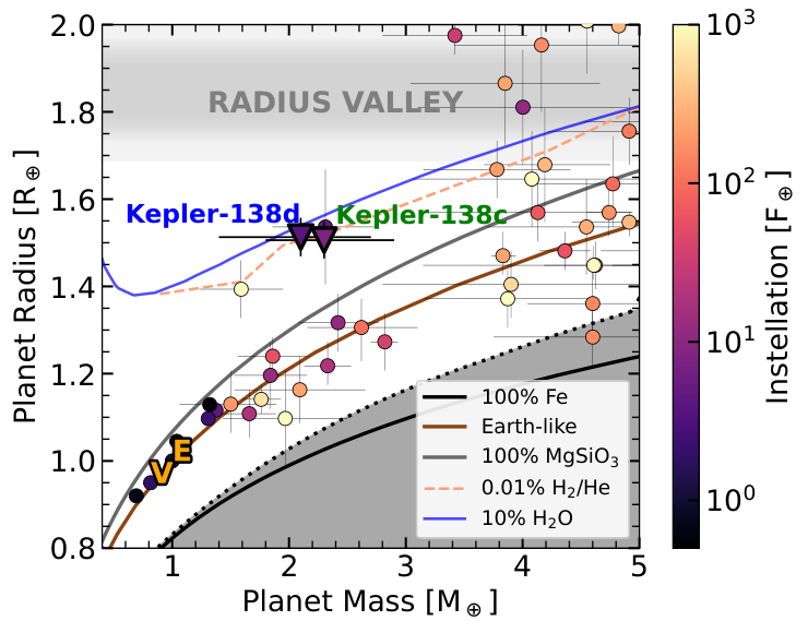


| Parameter | Unit | Value | Reference |
|---|---|---|---|
| Distance | pc | Ref. 133 | |
| Effective temperature, | K | Ref. 96 | |
| Metallicity, | dex | Ref. 96 | |
| Surface gravity, | cgs | This paper (derived) | |
| Stellar radius, | Ref. 55 | ||
| Stellar mass, | Ref. 55 | ||
| Stellar mean density, | g cm-3 | This paper (fitted) | |
| Stellar luminosity, | This paper (derived) |
| Parameter | Unit | Value |
|---|---|---|
| GP hyperparameters | ||
| Log covariance amplitude, | ||
| Log exponential timescale, | (days) | |
| Log coherence, | ||
| Periodic timescale, | (days) | |
| Additive jitter, | ||
| Planet parameters | ||
| Kepler-138 b | ||
| RV semi-amplitude, | ||
| Mass, | ||
| Kepler-138 c | ||
| RV semi-amplitude, | ||
| Mass, | ||
| Kepler-138 d | ||
| RV semi-amplitude, | ||
| Mass, | ||
| Kepler-138 e | ||
| RV semi-amplitude, | ||
| Mass, |
| Instrument | Wavelength | Depth | +1 | -1 |
|---|---|---|---|---|
| [m] | [ppm] | [ppm] | [ppm] | |
| Kepler | 0.43 – 0.88 | 630 | 35 | 35 |
| HST/WFC3 G141 | 1.11 – 1.23 | 651.6 | 43.4 | 43.0 |
| 1.23 – 1.35 | 670.3 | 37.7 | 37.6 | |
| 1.35 – 1.47 | 650.3 | 36.4 | 36.8 | |
| 1.47 – 1.59 | 632.2 | 37.4 | 37.7 | |
| Spitzer/IRAC Ch1 | 3.05 – 3.95 | 498.1 | 82.6 | 82.6 |
| Spitzer/IRAC Ch2 | 4.05 – 4.95 | 644.8 | 61.2 | 61.2 |
References
- 1 Rowe, J. F. et al. Validation of Kepler’s Multiple Planet Candidates. III. Light Curve Analysis and Announcement of Hundreds of New Multi-planet Systems. The Astrophysical Journal 784, 45 (2014). URL https://ui.adsabs.harvard.edu/abs/2014ApJ...784...45R. ADS Bibcode: 2014ApJ…784…45R.
- 2 Kipping, D. M. et al. The Hunt for Exomoons with Kepler (HEK). IV. A Search for Moons around Eight M Dwarfs. The Astrophysical Journal 784, 28 (2014). URL https://ui.adsabs.harvard.edu/2014ApJ...784...28K/abstract.
- 3 Jontof-Hutter, D., Rowe, J. F., Lissauer, J. J., Fabrycky, D. C. & Ford, E. B. The mass of the Mars-sized exoplanet Kepler-138 b from transit timing. Nature 522, 321 (2015). URL https://ui.adsabs.harvard.edu/2015Natur.522..321J/abstract.
- 4 Almenara, J. M., Díaz, R. F., Dorn, C., Bonfils, X. & Udry, S. Absolute densities in exoplanetary systems: photodynamical modelling of Kepler-138. Monthly Notices of the Royal Astronomical Society 478, 460 (2018). URL https://ui.adsabs.harvard.edu/2018MNRAS.478..460A/abstract.
- 5 Howard, A. W. et al. The California Planet Survey. I. Four New Giant Exoplanets. The Astrophysical Journal 721, 1467–1481 (2010). URL http://adsabs.harvard.edu/abs/2010ApJ...721.1467H.
- 6 Kopparapu, R. K. et al. Habitable Zones around Main-sequence Stars: New Estimates. The Astrophysical Journal 765, 131 (2013). URL http://adsabs.harvard.edu/abs/2013ApJ...765..131K.
- 7 Kubyshkina, D. et al. Grid of upper atmosphere models for 1-40 M⊕ planets: application to CoRoT-7 b and HD 219134 b,c. Astronomy and Astrophysics 619, A151 (2018). URL http://adsabs.harvard.edu/abs/2018A%26A...619A.151K.
- 8 Lammer, H. et al. Outgassing History and Escape of the Martian Atmosphere and Water Inventory. Space Science Reviews 174, 113–154 (2013). URL http://adsabs.harvard.edu/abs/2013SSRv..174..113L.
- 9 Dong, C., Jin, M. & Lingam, M. Atmospheric Escape From TOI-700 d: Venus vs. Earth Analogs. arXiv e-prints 2005, arXiv:2005.13190 (2020). URL http://adsabs.harvard.edu/abs/2020arXiv200513190D.
- 10 Khodachenko, M. L., Shaikhislamov, I. F., Lammer, H. & Prokopov, P. A. Atmosphere Expansion and Mass Loss of Close-orbit Giant Exoplanets Heated by Stellar XUV. II. Effects of Planetary Magnetic Field; Structuring of Inner Magnetosphere. The Astrophysical Journal 813, 50 (2015). URL https://ui.adsabs.harvard.edu/abs/2015ApJ...813...50K. ADS Bibcode: 2015ApJ…813…50K.
- 11 Kite, E. S. & Barnett, M. Exoplanet secondary atmosphere loss and revival. arXiv e-prints 2006, arXiv:2006.02589 (2020). URL http://adsabs.harvard.edu/abs/2020arXiv200602589K.
- 12 Bower, D. J., Hakim, K., Sossi, P. A. & Sanan, P. Retention of water in terrestrial magma oceans and carbon-rich early atmospheres. arXiv:2110.08029 [astro-ph] (2021). URL http://arxiv.org/abs/2110.08029. ArXiv: 2110.08029.
- 13 Aguichine, A., Mousis, O., Deleuil, M. & Marcq, E. Mass-radius relationships for irradiated ocean planets. arXiv e-prints 2105, arXiv:2105.01102 (2021). URL http://adsabs.harvard.edu/abs/2021arXiv210501102A.
- 14 Piaulet, C. et al. WASP-107b’s Density Is Even Lower: A Case Study for the Physics of Planetary Gas Envelope Accretion and Orbital Migration. The Astronomical Journal 161, 70 (2021). URL https://iopscience.iop.org/article/10.3847/1538-3881/abcd3c/meta. Publisher: IOP Publishing.
- 15 Bower, D. J. et al. Linking the evolution of terrestrial interiors and an early outgassed atmosphere to astrophysical observations. Astronomy and Astrophysics 631, A103 (2019). URL http://adsabs.harvard.edu/abs/2019A%26A...631A.103B.
- 16 Kite, E. S., Fegley, B., Jr., Schaefer, L. & Ford, E. B. Atmosphere Origins for Exoplanet Sub-Neptunes. The Astrophysical Journal 891, 111 (2020). URL http://adsabs.harvard.edu/abs/2020ApJ...891..111K.
- 17 Dorn, C. & Lichtenberg, T. Hidden water in magma ocean exoplanets. arXiv:2110.15069 [astro-ph] (2021). URL http://arxiv.org/abs/2110.15069. ArXiv: 2110.15069.
- 18 Luger, R. & Barnes, R. Extreme Water Loss and Abiotic O2Buildup on Planets Throughout the Habitable Zones of M Dwarfs. Astrobiology 15, 119–143 (2015). URL http://adsabs.harvard.edu/abs/2015AsBio..15..119L.
- 19 Lopez, E. D. Born dry in the photoevaporation desert: Kepler’s ultra-short-period planets formed water-poor. Monthly Notices of the Royal Astronomical Society 472, 245–253 (2017). URL http://adsabs.harvard.edu/abs/2017MNRAS.472..245L.
- 20 Kite, E. S. & Schaefer, L. Water on Hot Rocky Exoplanets. The Astrophysical Journal 909, L22 (2021). URL https://ui.adsabs.harvard.edu/abs/2021ApJ...909L..22K. ADS Bibcode: 2021ApJ…909L..22K.
- 21 Kuchner, M. J. Volatile-rich Earth-Mass Planets in the Habitable Zone. The Astrophysical Journal Letters 596, L105–L108 (2003). URL http://adsabs.harvard.edu/abs/2003ApJ...596L.105K.
- 22 Huang, S. & Ormel, C. W. The dynamics of the TRAPPIST-1 system in the context of its formation. arXiv:2109.10984 [astro-ph] (2021). URL http://arxiv.org/abs/2109.10984. ArXiv: 2109.10984.
- 23 Elkins-Tanton, L. T. & Seager, S. Ranges of Atmospheric Mass and Composition of Super-Earth Exoplanets. The Astrophysical Journal 685, 1237–1246 (2008). URL http://adsabs.harvard.edu/abs/2008ApJ...685.1237E.
- 24 Luger, R. et al. Habitable Evaporated Cores: Transforming Mini-Neptunes into Super-Earths in the Habitable Zones of M Dwarfs. AsBio 15, 57–88 (2015). URL https://ui.adsabs.harvard.edu/abs/2015AsBio..15...57L/abstract.
- 25 Weiss, L. M. & Marcy, G. W. The Mass-Radius Relation for 65 Exoplanets Smaller than 4 Earth Radii. The Astrophysical Journal Letters 783, L6 (2014). URL http://adsabs.harvard.edu/abs/2014ApJ...783L...6W.
- 26 Lundkvist, M. S. et al. Hot super-Earths stripped by their host stars. Nature Communications 7, 11201 (2016). URL http://adsabs.harvard.edu/abs/2016NatCo...711201L.
- 27 Otegi, J. F., Bouchy, F. & Helled, R. Revisited mass-radius relations for exoplanets below 120 M . Astronomy & Astrophysics 634, A43 (2020). URL https://www.aanda.org/10.1051/0004-6361/201936482.
- 28 Gupta, A. & Schlichting, H. E. Sculpting the valley in the radius distribution of small exoplanets as a by-product of planet formation: the core-powered mass-loss mechanism. Monthly Notices of the Royal Astronomical Society 487, 24–33 (2019). URL http://adsabs.harvard.edu/abs/2019MNRAS.487...24G.
- 29 Lee, E. J. & Chiang, E. Breeding Super-Earths and Birthing Super-puffs in Transitional Disks. The Astrophysical Journal 817, 90 (2016). URL https://ui.adsabs.harvard.edu/abs/2016ApJ...817...90L/abstract.
- 30 Owen, J. E. & Wu, Y. Kepler Planets: A Tale of Evaporation. The Astrophysical Journal 775, 105 (2013). URL http://adsabs.harvard.edu/abs/2013ApJ...775..105O.
- 31 Lopez, E. D. & Fortney, J. J. The Role of Core Mass in Controlling Evaporation: The Kepler Radius Distribution and the Kepler-36 Density Dichotomy. The Astrophysical Journal 776, 2 (2013). URL https://ui.adsabs.harvard.edu/abs/2013ApJ...776....2L.
- 32 Mills, S. M. & Mazeh, T. The Planetary Mass-Radius Relation and Its Dependence on Orbital Period as Measured by Transit Timing Variations and Radial Velocities. The Astrophysical Journal 839, L8 (2017). URL https://ui.adsabs.harvard.edu/abs/2017ApJ...839L...8M.
- 33 Bitsch, B., Raymond, S. N. & Izidoro, A. Rocky super-Earths or waterworlds: the interplay of planet migration, pebble accretion, and disc evolution. Astronomy & Astrophysics, Volume 624, id.A109, <NUMPAGES>12</NUMPAGES> pp. 624, A109 (2019). URL https://ui.adsabs.harvard.edu/abs/2019A%26A...624A.109B/abstract.
- 34 Benneke, B. et al. A sub-Neptune exoplanet with a low-metallicity methane-depleted atmosphere and Mie-scattering clouds. Nature Astronomy 3, 813–821 (2019). URL http://adsabs.harvard.edu/abs/2019NatAs...3..813B.
- 35 Benneke, B. et al. Water Vapor and Clouds on the Habitable-zone Sub-Neptune Exoplanet K2-18b. The Astrophysical Journal Letters 887, L14 (2019). URL http://adsabs.harvard.edu/abs/2019ApJ...887L..14B.
- 36 Deming, D. et al. INFRARED TRANSMISSION SPECTROSCOPY OF THE EXOPLANETS HD 209458b AND XO-1b USING THE WIDE FIELD CAMERA-3 ON THE HUBBLE SPACE TELESCOPE. The Astrophysical Journal 774, 95 (2013). URL http://stacks.iop.org/0004-637X/774/i=2/a=95?key=crossref.fd5770b405c343912aaffa1347d1a6b3.
- 37 Tsiaras, A. et al. A New Approach to Analyzing HST Spatial Scans: The Transmission Spectrum of HD 209458 b. The Astrophysical Journal 832, 202 (2016). URL http://adsabs.harvard.edu/abs/2016ApJ...832..202T.
- 38 Grillmair, C. J. et al. Pointing effects and their consequences for Spitzer IRAC exoplanet observations 8448, 84481I (2012). URL http://adsabs.harvard.edu/abs/2012SPIE.8448E..1IG. Conference Name: Observatory Operations: Strategies, Processes, and Systems IV.
- 39 Benneke, B. et al. Spitzer Observations Confirm and Rescue the Habitable-zone Super-Earth K2-18b for Future Characterization. The Astrophysical Journal 834, 187 (2017). URL http://adsabs.harvard.edu/abs/2017ApJ...834..187B.
- 40 Foreman-Mackey, D., Hogg, D. W., Lang, D. & Goodman, J. emcee: The MCMC Hammer. Publications of the Astronomical Society of the Pacific 125, 306 (2013). URL http://adsabs.harvard.edu/abs/2013PASP..125..306F.
- 41 Kreidberg, L. batman: BAsic Transit Model cAlculatioN in Python. PASP 127, 1161 (2015). 1507.08285.
- 42 Parviainen, H. & Aigrain, S. LDTK: Limb Darkening Toolkit. Monthly Notices of the Royal Astronomical Society 453, 3821–3826 (2015). URL http://adsabs.harvard.edu/abs/2015MNRAS.453.3821P.
- 43 Sing, D. K. Stellar limb-darkening coefficients for CoRot and Kepler. Astronomy and Astrophysics 510, A21 (2010). URL http://adsabs.harvard.edu/abs/2010A%26A...510A..21S.
- 44 Kreidberg, L. et al. Clouds in the atmosphere of the super-Earth exoplanet GJ1214b. Nature 505, 69–72 (2014). URL http://adsabs.harvard.edu/abs/2014Natur.505...69K.
- 45 Kreidberg, L. et al. A Detection of Water in the Transmission Spectrum of the Hot Jupiter WASP-12b and Implications for Its Atmospheric Composition. The Astrophysical Journal 814, 66 (2015). URL http://adsabs.harvard.edu/abs/2015ApJ...814...66K.
- 46 Deming, D. et al. Spitzer Secondary Eclipses of the Dense, Modestly-irradiated, Giant Exoplanet HAT-P-20b Using Pixel-level Decorrelation. The Astrophysical Journal 805, 132 (2015). URL http://adsabs.harvard.edu/abs/2015ApJ...805..132D.
- 47 Stevenson, K. B. et al. Transit and Eclipse Analyses of the Exoplanet HD 149026b Using BLISS Mapping. The Astrophysical Journal 754, 136 (2012). URL http://adsabs.harvard.edu/abs/2012ApJ...754..136S.
- 48 Ragozzine, D. & Holman, M. J. The Value of Systems with Multiple Transiting Planets. arXiv e-prints arXiv:1006.3727 (2010). URL https://ui.adsabs.harvard.edu/abs/2010arXiv1006.3727R.
- 49 Agol, E. et al. Refining the transit timing and photometric analysis of TRAPPIST-1: Masses, radii, densities, dynamics, and ephemerides. arXiv e-prints 2010, arXiv:2010.01074 (2020). URL http://adsabs.harvard.edu/abs/2020arXiv201001074A.
- 50 Jontof-Hutter, D. et al. Following up the Kepler field: Masses of Targets for transit timing and atmospheric characterization. arXiv:2101.01202 [astro-ph] (2021). URL http://arxiv.org/abs/2101.01202. ArXiv: 2101.01202.
- 51 Deck, K. M., Agol, E., Holman, M. J. & Nesvorný, D. TTVFast: An Efficient and Accurate Code for Transit Timing Inversion Problems. The Astrophysical Journal 787, 132 (2014). URL http://adsabs.harvard.edu/abs/2014ApJ...787..132D.
- 52 Ford, E. B. Improving the Efficiency of Markov Chain Monte Carlo for Analyzing the Orbits of Extrasolar Planets. The Astrophysical Journal 642, 505–522 (2006). URL http://adsabs.harvard.edu/abs/2006ApJ...642..505F.
- 53 Mann, A. W., Feiden, G. A., Gaidos, E., Boyajian, T. & von Braun, K. How to Constrain Your M Dwarf: Measuring Effective Temperature, Bolometric Luminosity, Mass, and Radius. The Astrophysical Journal 804, 64 (2015). URL http://adsabs.harvard.edu/abs/2015ApJ...804...64M.
- 54 Mann, A. W. et al. How to Constrain Your M Dwarf. II. The Mass-Luminosity-Metallicity Relation from 0.075 to 0.70 Solar Masses. The Astrophysical Journal 871, 63 (2019). URL http://adsabs.harvard.edu/abs/2019ApJ...871...63M.
- 55 Berger, T. A. et al. The Gaia-Kepler Stellar Properties Catalog. I. Homogeneous Fundamental Properties for 186,301 Kepler Stars. arXiv:2001.07737 [astro-ph] (2020). URL http://arxiv.org/abs/2001.07737. ArXiv: 2001.07737.
- 56 Goodman, J. & Weare, J. Ensemble samplers with affine invariance. Communications in Applied Mathematics and Computational Science 5, 65–80 (2010). URL https://msp.org/camcos/2010/5-1/p04.xhtml. Publisher: Mathematical Sciences Publishers.
- 57 Nelson, B. E., Ford, E. B. & Payne, M. J. RUN DMC: An efficient, parallel code for analyzing Radial Velocity Observations using N-body Integrations and Differential Evolution Markov chain Monte Carlo. The Astrophysical Journal Supplement Series 210, 11 (2013). URL http://arxiv.org/abs/1311.5229. ArXiv:1311.5229 [astro-ph].
- 58 Heyl, J. S. & Gladman, B. J. Using long-term transit timing to detect terrestrial planets. Monthly Notices of the Royal Astronomical Society 377, 1511–1519 (2007). URL http://adsabs.harvard.edu/abs/2007MNRAS.377.1511H.
- 59 Rein, H. & Liu, S.-F. REBOUND: an open-source multi-purpose N-body code for collisional dynamics. Astronomy and Astrophysics 537, A128 (2012). URL http://adsabs.harvard.edu/abs/2012A%26A...537A.128R.
- 60 Rein, H. & Tamayo, D. WHFAST: a fast and unbiased implementation of a symplectic Wisdom-Holman integrator for long-term gravitational simulations. Monthly Notices of the Royal Astronomical Society 452, 376–388 (2015). URL http://adsabs.harvard.edu/abs/2015MNRAS.452..376R.
- 61 Mandel, K. & Agol, E. Analytic Light Curves for Planetary Transit Searches. The Astrophysical Journal Letters 580, L171–L175 (2002). URL http://adsabs.harvard.edu/abs/2002ApJ...580L.171M.
- 62 Wang, J., Fischer, D. A., Xie, J.-W. & Ciardi, D. R. Influence of Stellar Multiplicity on Planet Formation. IV. Adaptive Optics Imaging of Kepler Stars with Multiple Transiting Planet Candidates. The Astrophysical Journal 813, 130 (2015). URL https://ui.adsabs.harvard.edu/abs/2015ApJ...813..130W. ADS Bibcode: 2015ApJ…813..130W.
- 63 Vogt, S. S. et al. HIRES: the high-resolution echelle spectrometer on the Keck 10-m Telescope 2198, 362 (1994). URL http://adsabs.harvard.edu/abs/1994SPIE.2198..362V. Conference Name: Instrumentation in Astronomy VIII.
- 64 Butler, R. P. et al. Attaining Doppler Precision of 3 M s-1. Publications of the Astronomical Society of the Pacific 108, 500 (1996). URL http://adsabs.harvard.edu/abs/1996PASP..108..500B.
- 65 Fulton, B. J., Petigura, E. A., Blunt, S. & Sinukoff, E. RadVel: The Radial Velocity Modeling Toolkit. Publications of the Astronomical Society of the Pacific 130, 044504 (2018). URL https://ui.adsabs.harvard.edu/abs/2018PASP..130d4504F/abstract.
- 66 Amado, P. J. et al. The CARMENES search for exoplanets around M dwarfs. Two terrestrial planets orbiting G 264-012 and one terrestrial planet orbiting Gl 393. arXiv e-prints 2105, arXiv:2105.13785 (2021). URL http://adsabs.harvard.edu/abs/2021arXiv210513785A.
- 67 Ahrer, E. et al. The HARPS search for southern extra-solar planets XLV. Two Neptune mass planets orbiting HD 13808: a study of stellar activity modelling’s impact on planet detection. arXiv e-prints 2102, arXiv:2102.03387 (2021). URL http://adsabs.harvard.edu/abs/2021arXiv210203387A.
- 68 Ambikasaran, S., Foreman-Mackey, D., Greengard, L., Hogg, D. W. & O’Neil, M. Fast Direct Methods for Gaussian Processes. IEEE Transactions on Pattern Analysis and Machine Intelligence 38 (2015). URL http://adsabs.harvard.edu/abs/2015ITPAM..38..252A.
- 69 McQuillan, A., Aigrain, S. & Mazeh, T. Measuring the rotation period distribution of field M dwarfs with Kepler. Monthly Notices of the Royal Astronomical Society 432, 1203–1216 (2013). URL http://adsabs.harvard.edu/abs/2013MNRAS.432.1203M.
- 70 McQuillan, A., Mazeh, T. & Aigrain, S. Stellar Rotation Periods of the Kepler Objects of Interest: A Dearth of Close-in Planets around Fast Rotators. The Astrophysical Journal Letters 775, L11 (2013). URL http://adsabs.harvard.edu/abs/2013ApJ...775L..11M.
- 71 Benneke, B. Strict Upper Limits on the Carbon-to-Oxygen Ratios of Eight Hot Jupiters from Self-Consistent Atmospheric Retrieval. arXiv e-prints 1504, arXiv:1504.07655 (2015). URL http://adsabs.harvard.edu/abs/2015arXiv150407655B.
- 72 Benneke, B. & Seager, S. Atmospheric Retrieval for Super-Earths: Uniquely Constraining the Atmospheric Composition with Transmission Spectroscopy. The Astrophysical Journal 753, 100 (2012). URL http://adsabs.harvard.edu/abs/2012ApJ...753..100B.
- 73 Benneke, B. & Seager, S. How to Distinguish between Cloudy Mini-Neptunes and Water/Volatile-dominated Super-Earths. The Astrophysical Journal 778, 153 (2013). URL http://adsabs.harvard.edu/abs/2013ApJ...778..153B.
- 74 Feroz, F., Hobson, M. P. & Bridges, M. MULTINEST: an efficient and robust Bayesian inference tool for cosmology and particle physics. Monthly Notices of the Royal Astronomical Society 398, 1601–1614 (2009). URL http://adsabs.harvard.edu/abs/2009MNRAS.398.1601F.
- 75 Shaw, J. R., Bridges, M. & Hobson, M. P. Efficient Bayesian inference for multimodal problems in cosmology. Monthly Notices of the Royal Astronomical Society 378, 1365–1370 (2007). URL https://ui.adsabs.harvard.edu/abs/2007MNRAS.378.1365S.
- 76 Mukherjee, P., Parkinson, D. & Liddle, A. R. A Nested Sampling Algorithm for Cosmological Model Selection. The Astrophysical Journal 638, L51–L54 (2006). URL https://ui.adsabs.harvard.edu/abs/2006ApJ...638L..51M.
- 77 Skilling, J. Nested Sampling 735, 395–405 (2004). URL http://adsabs.harvard.edu/abs/2004AIPC..735..395S. Conference Name: Bayesian Inference and Maximum Entropy Methods in Science and Engineering: 24th International Workshop on Bayesian Inference and Maximum Entropy Methods in Science and Engineering.
- 78 Trotta, R. Bayes in the sky: Bayesian inference and model selection in cosmology. Contemporary Physics 49, 71 (2008). URL https://ui.adsabs.harvard.edu/abs/2008ConPh..49...71T/abstract.
- 79 Line, M. R. & Parmentier, V. The Influence of Nonuniform Cloud Cover on Transit Transmission Spectra. The Astrophysical Journal 820, 78 (2016). URL http://adsabs.harvard.edu/abs/2016ApJ...820...78L.
- 80 Miller-Ricci, E., Seager, S. & Sasselov, D. The Atmospheric Signatures of Super-Earths: How to Distinguish Between Hydrogen-Rich and Hydrogen-Poor Atmospheres. The Astrophysical Journal 690, 1056–1067 (2009). URL http://adsabs.harvard.edu/abs/2009ApJ...690.1056M.
- 81 Thorngren, D., Gao, P. & Fortney, J. J. The Intrinsic Temperature and Radiative-Convective Boundary Depth in the Atmospheres of Hot Jupiters. The Astrophysical Journal Letters 884, L6 (2019). URL http://adsabs.harvard.edu/abs/2019ApJ...884L...6T.
- 82 Chabrier, G., Mazevet, S. & Soubiran, F. A New Equation of State for Dense Hydrogen-Helium Mixtures. The Astrophysical Journal 872, 51 (2019). URL http://adsabs.harvard.edu/abs/2019ApJ...872...51C.
- 83 Mazevet, S., Licari, A., Chabrier, G. & Potekhin, A. Y. Ab initio based equation of state of dense water for planetary and exoplanetary modeling. Astronomy and Astrophysics 621, A128 (2019). URL http://adsabs.harvard.edu/abs/2019A%26A...621A.128M.
- 84 Valencia, D., Guillot, T., Parmentier, V. & Freedman, R. S. BULK COMPOSITION OF GJ 1214b AND OTHER SUB-NEPTUNE EXOPLANETS. The Astrophysical Journal 775, 10 (2013). URL https://iopscience.iop.org/article/10.1088/0004-637X/775/1/10.
- 85 Madhusudhan, N., Nixon, M. C., Welbanks, L., Piette, A. A. A. & Booth, R. A. The Interior and Atmosphere of the Habitable-zone Exoplanet K2-18b. The Astrophysical Journal Letters 891, L7 (2020). URL http://adsabs.harvard.edu/abs/2020ApJ...891L...7M.
- 86 Lopez, E. D. & Fortney, J. J. Understanding the Mass-Radius Relation for Sub-neptunes: Radius as a Proxy for Composition. The Astrophysical Journal 792, 1 (2014). URL http://adsabs.harvard.edu/abs/2014ApJ...792....1L.
- 87 Hubbard, W. B. et al. Theory of Extrasolar Giant Planet Transits. The Astrophysical Journal 560, 413–419 (2001). URL https://ui.adsabs.harvard.edu/abs/2001ApJ...560..413H. ADS Bibcode: 2001ApJ…560..413H.
- 88 Otegi, J. F. et al. Impact of the measured parameters of exoplanets on the inferred internal structure. Astronomy & Astrophysics, Volume 640, id.A135, <NUMPAGES>12</NUMPAGES> pp. 640, A135 (2020). URL https://ui.adsabs.harvard.edu/abs/2020A%26A...640A.135O/abstract.
- 89 Lozovsky, M., Helled, R., Dorn, C. & Venturini, J. Threshold Radii of Volatile-rich Planets. The Astrophysical Journal 866, 49 (2018). URL https://iopscience.iop.org/article/10.3847/1538-4357/aadd09.
- 90 Turbet, M., Ehrenreich, D., Lovis, C., Bolmont, E. & Fauchez, T. The runaway greenhouse radius inflation effect. An observational diagnostic to probe water on Earth-sized planets and test the habitable zone concept. Astronomy and Astrophysics 628, A12 (2019). URL http://adsabs.harvard.edu/abs/2019A%26A...628A..12T.
- 91 Turbet, M. et al. Revised mass-radius relationships for water-rich rocky planets more irradiated than the runaway greenhouse limit. Astronomy & Astrophysics, Volume 638, id.A41, <NUMPAGES>10</NUMPAGES> pp. 638, A41 (2020). URL https://ui.adsabs.harvard.edu/abs/2020A%26A...638A..41T/abstract.
- 92 Zeng, L., Sasselov, D. D. & Jacobsen, S. B. Mass-Radius Relation for Rocky Planets Based on PREM. The Astrophysical Journal 819, 127 (2016). URL http://adsabs.harvard.edu/abs/2016ApJ...819..127Z.
- 93 Madhusudhan, N., Piette, A. A. A. & Constantinou, S. Habitability and Biosignatures of Hycean Worlds. The Astrophysical Journal 918, 1 (2021). URL https://ui.adsabs.harvard.edu/abs/2021ApJ...918....1M. ADS Bibcode: 2021ApJ…918….1M.
- 94 Kosiarek, M. R. et al. Physical Parameters of the Multi-Planet Systems HD 106315 and GJ 9827. arXiv:2009.03398 [astro-ph] (2020). URL http://arxiv.org/abs/2009.03398. ArXiv: 2009.03398.
- 95 Curtis, J. L. et al. When Do Stalled Stars Resume Spinning Down? Advancing Gyrochronology with Ruprecht 147. The Astrophysical Journal 904, 140 (2020). URL https://ui.adsabs.harvard.edu/abs/2020ApJ...904..140C. ADS Bibcode: 2020ApJ…904..140C.
- 96 Muirhead, P. S. et al. Characterizing the Cool Kepler Objects of Interests. New Effective Temperatures, Metallicities, Masses, and Radii of Low-mass Kepler Planet-candidate Host Stars. The Astrophysical Journal 750, L37 (2012). URL https://ui.adsabs.harvard.edu/2012ApJ...750L..37M/abstract.
- 97 Watson, A. J., Donahue, T. M. & Walker, J. C. G. The dynamics of a rapidly escaping atmosphere: Applications to the evolution of Earth and Venus. Icarus 48, 150–166 (1981). URL https://ui.adsabs.harvard.edu/abs/1981Icar...48..150W. ADS Bibcode: 1981Icar…48..150W.
- 98 Owen, J. E. & Wu, Y. The Evaporation Valley in the Kepler Planets. The Astrophysical Journal 847, 29 (2017). URL http://adsabs.harvard.edu/abs/2017ApJ...847...29O.
- 99 Feinstein, A. D. et al. Flare Statistics for Young Stars from a Convolutional Neural Network Analysis of $\textit{TESS}$ Data. The Astronomical Journal 160, 219 (2020). URL http://arxiv.org/abs/2005.07710. ArXiv: 2005.07710.
- 100 Ribas, I., Guinan, E. F., Güdel, M. & Audard, M. Evolution of the Solar Activity over Time and Effects on Planetary Atmospheres. I. High-Energy Irradiances (1-1700 Å). The Astrophysical Journal 622, 680–694 (2005). URL http://adsabs.harvard.edu/abs/2005ApJ...622..680R.
- 101 Jackson, A. P., Davis, T. A. & Wheatley, P. J. The coronal X-ray-age relation and its implications for the evaporation of exoplanets. Monthly Notices of the Royal Astronomical Society 422, 2024–2043 (2012). URL http://adsabs.harvard.edu/abs/2012MNRAS.422.2024J.
- 102 Tu, L., Johnstone, C. P., Güdel, M. & Lammer, H. The extreme ultraviolet and X-ray Sun in Time: High-energy evolutionary tracks of a solar-like star. Astronomy and Astrophysics 577, L3 (2015). URL http://adsabs.harvard.edu/abs/2015A%26A...577L...3T.
- 103 Güdel, M., Guinan, E. F. & Skinner, S. L. The X-Ray Sun in Time: A Study of the Long-Term Evolution of Coronae of Solar-Type Stars. The Astrophysical Journal 483, 947–960 (1997). URL http://adsabs.harvard.edu/abs/1997ApJ...483..947G.
- 104 Murray-Clay, R. A., Chiang, E. I. & Murray, N. Atmospheric Escape From Hot Jupiters. The Astrophysical Journal 693, 23–42 (2009). URL http://adsabs.harvard.edu/abs/2009ApJ...693...23M.
- 105 Owen, J. E. & Jackson, A. P. Planetary evaporation by UV & X-ray radiation: basic hydrodynamics. Monthly Notices of the Royal Astronomical Society 425, 2931–2947 (2012). URL http://adsabs.harvard.edu/abs/2012MNRAS.425.2931O.
- 106 Owen, J. E. & Alvarez, M. A. UV Driven Evaporation of Close-in Planets: Energy-limited, Recombination-limited, and Photon-limited Flows. The Astrophysical Journal 816, 34 (2016). URL http://adsabs.harvard.edu/abs/2016ApJ...816...34O.
- 107 Erkaev, N. V. et al. EUV-driven mass-loss of protoplanetary cores with hydrogen-dominated atmospheres: the influences of ionization and orbital distance. Monthly Notices of the Royal Astronomical Society 460, 1300–1309 (2016). URL https://ui.adsabs.harvard.edu/abs/2016MNRAS.460.1300E. ADS Bibcode: 2016MNRAS.460.1300E.
- 108 Erkaev, N. V. et al. Roche lobe effects on the atmospheric loss from “Hot Jupiters”. Astronomy and Astrophysics 472, 329–334 (2007). URL http://adsabs.harvard.edu/abs/2007A%26A...472..329E.
- 109 Johnstone, C. P., Bartel, M. & Güdel, M. The active lives of stars: A complete description of the rotation and XUV evolution of F, G, K, and M dwarfs. Astronomy and Astrophysics 649, A96 (2021). URL https://ui.adsabs.harvard.edu/abs/2021A&A...649A..96J/abstract.
- 110 Schaefer, L. & Fegley, B. Chemistry of atmospheres formed during accretion of the Earth and other terrestrial planets. Icarus 208, 438–448 (2010). URL http://adsabs.harvard.edu/abs/2010Icar..208..438S.
- 111 Lichtenberg, T. et al. Vertically resolved magma ocean-protoatmosphere evolution: H$_2$, H$_2$O, CO$_2$, CH$_4$, CO, O$_2$, and N$_2$ as primary absorbers. Journal of Geophysical Research: Planets (2021). URL http://arxiv.org/abs/2101.10991. ArXiv: 2101.10991.
- 112 Sossi, P. A. Atmospheres in the baking. Nature Astronomy 5, 535–536 (2021). URL https://ui.adsabs.harvard.edu/abs/2021NatAs...5..535S. ADS Bibcode: 2021NatAs…5..535S.
- 113 Andrault, D., Monteux, J., Le Bars, M. & Samuel, H. The deep Earth may not be cooling down. Earth and Planetary Science Letters, Volume 443, p. 195-203. 443, 195 (2016). URL https://ui.adsabs.harvard.edu/abs/2016E%26PSL.443..195A/abstract.
- 114 Rackham, B. V., Apai, D. & Giampapa, M. S. The Transit Light Source Effect: False Spectral Features and Incorrect Densities for M-dwarf Transiting Planets. The Astrophysical Journal 853, 122 (2018). URL http://adsabs.harvard.edu/abs/2018ApJ...853..122R.
- 115 Husser, T.-O. et al. A new extensive library of PHOENIX stellar atmospheres and synthetic spectra. Astronomy & Astrophysics, Volume 553, id.A6, <NUMPAGES>9</NUMPAGES> pp. 553, A6 (2013). URL https://ui.adsabs.harvard.edu/abs/2013A%26A...553A...6H/abstract.
- 116 Gao, P. & Zhang, X. Deflating Super-puffs: Impact of Photochemical Hazes on the Observed Mass-Radius Relationship of Low-mass Planets. The Astrophysical Journal 890, 93 (2020). URL http://adsabs.harvard.edu/abs/2020ApJ...890...93G.
- 117 Lavvas, P., Koskinen, T., Steinrueck, M. E., García Muñoz, A. & Showman, A. P. Photochemical Hazes in Sub-Neptunian Atmospheres with a Focus on GJ 1214b. The Astrophysical Journal 878, 118 (2019). URL http://adsabs.harvard.edu/abs/2019ApJ...878..118L.
- 118 Piro, A. L. Can Rocky Exoplanets with Rings Pose as Sub-Neptunes? The Astronomical Journal 156, 80 (2018). URL http://adsabs.harvard.edu/abs/2018AJ....156...80P.
- 119 Piro, A. L. & Vissapragada, S. Exploring Whether Super-Puffs Can Be Explained as Ringed Exoplanets. The Astronomical Journal 159, 131 (2020). URL http://arxiv.org/abs/1911.09673. ArXiv: 1911.09673.
- 120 Clausen, N. & Tilgner, A. Dissipation in rocky planets for strong tidal forcing. Astronomy and Astrophysics 584, A60 (2015). URL http://adsabs.harvard.edu/abs/2015A%26A...584A..60C.
- 121 Chandrasekhar, S. Ellipsoidal figures of equilibrium. The Silliman Foundation Lectures, New Haven: Yale University Press, 1969 (1969). URL http://adsabs.harvard.edu/abs/1969efe..book.....C.
- 122 Tremaine, S., Touma, J. & Namouni, F. Satellite Dynamics on the Laplace Surface. The Astronomical Journal 137, 3706–3717 (2009). URL http://adsabs.harvard.edu/abs/2009AJ....137.3706T.
- 123 Schlichting, H. E. & Chang, P. Warm Saturns: On the Nature of Rings around Extrasolar Planets That Reside inside the Ice Line. The Astrophysical Journal 734, 117 (2011). URL http://adsabs.harvard.edu/abs/2011ApJ...734..117S.
- 124 Astropy Collaboration et al. Astropy: A community Python package for astronomy. A&A 558, A33 (2013). 1307.6212.
- 125 Astropy Collaboration et al. The Astropy Project: Building an Open-science Project and Status of the v2.0 Core Package. AJ 156, 123 (2018). 1801.02634.
- 126 Harris, C. R. et al. Array programming with NumPy. Nature 585, 357–362 (2020). URL https://doi.org/10.1038/s41586-020-2649-2.
- 127 Pérez, F. & Granger, B. E. Ipython: a system for interactive scientific computing (2007).
- 128 Hunter, J. D. Matplotlib: A 2d graphics environment. Computing in Science & Engineering 9, 90–95 (2007).
- 129 Tange, O. Gnu parallel 20200722 (’privacy shield’) (2020). URL https://doi.org/10.5281/zenodo.3956817. GNU Parallel is a general parallelizer to run multiple serial command line programs in parallel without changing them.
- 130 Zeng, L. & Sasselov, D. A Detailed Model Grid for Solid Planets from 0.1 through 100 Earth Masses. Publications of the Astronomical Society of the Pacific 125, 227 (2013). URL http://adsabs.harvard.edu/abs/2013PASP..125..227Z.
- 131 Marcus, R. A., Sasselov, D., Hernquist, L. & Stewart, S. T. Minimum Radii of Super-Earths: Constraints from Giant Impacts. The Astrophysical Journal Letters 712, L73–L76 (2010). URL http://adsabs.harvard.edu/abs/2010ApJ...712L..73M.
- 132 Lu, Y. L., Angus, R., Curtis, J. L., David, T. J. & Kiman, R. Gyro-kinematic Ages for around 30,000 Kepler Stars. The Astronomical Journal 161, 189 (2021). URL https://ui.adsabs.harvard.edu/abs/2021AJ....161..189L. ADS Bibcode: 2021AJ….161..189L.
- 133 Bailer-Jones, C. A. L., Rybizki, J., Fouesneau, M., Mantelet, G. & Andrae, R. Estimating Distance from Parallaxes. IV. Distances to 1.33 Billion Stars in Gaia Data Release 2. The Astronomical Journal 156, 58 (2018). URL https://ui.adsabs.harvard.edu/abs/2018AJ....156...58B.