Neural Enhanced Belief Propagation
for Multiobject Tracking
Abstract
Algorithmic solutions for mot (mot) are a key enabler for applications in autonomous navigation and applied ocean sciences. State-of-the-art mot methods fully rely on a statistical model and typically use preprocessed sensor data as measurements. In particular, measurements are produced by a detector that extracts potential object locations from the raw sensor data collected for a discrete time step. This preparatory processing step reduces data flow and computational complexity but may result in a loss of information. State-of-the-art Bayesian mot methods that are based on belief propagation ( bp (bp)) systematically exploit graph structures of the statistical model to reduce computational complexity and improve scalability. However, as a fully model-based approach, BP can only provide suboptimal estimates when there is a mismatch between the statistical model and the true data-generating process. Existing BP-based mot methods can further only make use of preprocessed measurements. In this paper, we introduce a variant of BP that combines model-based with data-driven mot. The proposed nebp (nebp) method complements the statistical model of BP by information learned from raw sensor data. This approach conjectures that the learned information can reduce model mismatch and thus improve data association and false alarm rejection. Our NEBP method improves tracking performance compared to model-based methods. At the same time, it inherits the advantages of bp-based mot, i.e., it scales only quadratically in the number of objects, and it can thus generate and maintain a large number of object tracks. We evaluate the performance of our nebp approach for mot on the nuScenes autonomous driving dataset and demonstrate that it has state-of-the-art performance.
Index Terms:
Multiobject tracking, belief propagation, probabilistic data association, factor graphs, graph neural networksI Introduction
Multi-object tracking (mot) [1, 2, 3, 4, 5, 6, 7, 8, 9, 10, 11, 12, 13, 14, 15, 16, 17, 18, 19, 20, 21, 22, 23] enables emerging applications including autonomous driving, applied ocean sciences, and indoor localization. mot aims at estimating the states (e.g., positions and possibly other parameters) of moving objects over time, based on measurements provided by sensing technologies such as Light Detection and Ranging (LiDAR), radar, or sonar [1, 2, 3, 4, 5, 6, 7, 8, 9, 10, 11, 12, 13, 14, 15, 16, 17, 18, 19, 20, 21, 22, 23]. An inherent problem in mot is measurement-origin uncertainty, i.e., the unknown association between measurements and objects. mot is further complicated by the fact that the number of objects is unknown, i.e., for the initialization and termination of object tracks, track management schemes need to be employed.
I-A Model-Based and Data-Driven MOT
Typically mot methods rely on measurements that have been extracted from raw sensor data in a detection process. For example, an object detector [24, 25, 26, 27, 28, 29] can be applied to LiDAR scans or images at each time step independently, and the detected objects are then used as measurements for mot [30, 31]. This common strategy is referred to as “detect-then-track”. Based on the assumption that, at each time step, an object can generate at most one measurement and each measurement can be originated by at most one object, data association can be cast as a bipartite matching problem.
The first class of mot methods follows a global nearest neighbor association approach [1]. Here, a Hungarian [32] or a greedy matching algorithm is used to perform “hard” measurement-to-object associations [16, 21, 15, 22, 17, 18, 19, 20]. To improve the reliability of hard associations, these methods often rely on discriminative shape information of objects and measurements. Shape information is extracted from raw sensor data based on deep neural networks [22, 21] and used to compute pairwise distances between objects and measurements more accurately. The methods in this class typically rely on heuristics for track management.
A second class of methods formulates and solves the mot problem in the Bayesian estimation framework [1, 2, 6, 5, 7, 8, 10, 3, 4, 12]. Methods in this class rely on a statistical model for object birth, object motion, and measurement generation [1, 2, 6, 5, 7, 8, 10, 3, 4, 12]. The statistical model makes it possible to perform a more robust probabilistic “soft” data association and to avoid heuristics for track initialization and termination. Methods in this class include the jpda (jpda) filter [1], the mht (mht) [33], rfs (rfs) filters [6, 7, 8, 10, 11], and bp-based mot [6, 3, 4, 5].
bp, also known as the sum-product algorithm, [34, 35, 36] provides an efficient and scalable solution to high-dimensional inference problems. bp operates by “passing messages” along the edges of the factor graph [34] that represents the statistical model of the inference problem. Important algorithms such as the Kalman filter, the particle filter [37], and the jpda filter [1] are instances of bp. By exploiting the structure of the graph, bp-based mot methods [6, 3, 4, 5] are highly scalable. In particular, using BP, “soft” probabilistic data association can be performed for hundreds of objects. This makes it possible to generate and maintain a very large number of potential object tracks and, in turn, achieve state-of-the-art mot performance [6, 3, 4, 5].
Existing bp-based methods entirely rely on “hand-designed” statistical models. However, the statistical models are often unable to accurately represent all the intricate details of the true data-generating process. This mismatch leads to suboptimal object state estimates. In addition, since bp methods rely on the detect-then-track strategy, important object-related information might be discarded by the object detector. On the other hand, learning-based methods are fully data-driven, i.e., they do not make use of any statistical model. Typically, learning-based methods rely on deep neural networks, which facilitate the extraction of all relevant information from raw sensor data [21, 22]. However, learning-based mot typically makes use of potentially unreliable heuristics for track management and only performs well in “big data” problems.
A graph neural network (GNN) [38, 39] is a graphical model formed by neural networks. The neural network “passes messages”, i.e., exchange processing results, along the edges of the GNN. This mechanism is similar to the message passing performed by BP. It has been demonstrated that in Bayesian estimation problems, a GNN can outperform loopy BP [40] if sufficient training data is available. Recently, neural enhanced belief propagation (NEBP) [41] was introduced. In nebp, a gnn (gnn) [38, 39] that matches the topology of the factor graph is established. After training the GNN, the GNN messages can complement the corresponding BP messages to correct errors introduced by cycles and model mismatch. The resulting hybrid message passing method combines the benefits of model-based and data-driven inference. In particular, NEBP can leverage the performance advantages of GNNs in big data problems. The benefits of NEBP have been demonstrated in decoding [41] and cooperative localization [42] problems.
I-B Contribution and Paper Organization
In this paper, we address the fundamental question of how model-based and data-driven approaches can be combined in a hybrid inference method. In particular, we aim to develop a bp-based mot method that augments its “hand-designed” statistical model with information learned from raw sensor data. As a result, we propose nebp for mot. Here, BP messages calculated for probabilistic data association are combined with the output of a gnn. The gnn uses object detections and features learned from raw sensor information as inputs. It can improve the MOT performance of BP by introducing data-driven false alarm rejection and object shape association.
False alarm rejection aims at identifying which measurements are likely false alarms. For measurements that have been identified as a potential false alarm, the false alarm distribution in the statistical model used by bp is locally increased. This reduces the probability that the measurement is associated with an existing object track or initializes a new object track. Object shape association computes improved association probabilities by also taking features of existing object tracks and measurements that have been learned from raw sensor data into account. Compared to bp for mot, the resulting nebp method for mot can improve object declaration and estimation performance if annotated data is available, and consequently provide state-of-the-art performance in big data mot problems.
The key contributions of this paper are summarized as follows.
- •
We introduce nebp for mot where probabilistic data association is enhanced by learned information provided by a gnn.
- •
We present the procedure and the loss function, used for the training of the gnn, that enable false alarm rejection and object shape association.
- •
We apply the proposed method to an autonomous driving dataset and demonstrate state-of-the-art object tracking performance.
An overview of the proposed nebp method for mot is presented as a flow diagram in Fig. 1. Here, black boxes show the computation modules performed by both conventional bp and nebp. The red boxes show the additional modules only performed by the proposed nebp method. A detailed description of each module will be provided in Sections IV and V.
In modern MOT scenarios with high-resolution sensors, it is often challenging to capture object shapes and the corresponding data-generating process by a statistical model. Thus, in contrast to the extended object tracking strategy [43, 44, 5], the influence of object shapes on data generation is best learned directly from data. This paper advances over the preliminary account of our method provided in the conference publication [45] by (i) introducing a new factor graph representation, which is a more accurate description of the proposed nebp method; (ii) presenting more details on the development and implementation of the proposed nebp approach for mot; and (iii) conducting a comprehensive evaluation based on real data that highlights why NEBP advances BP in MOT applications, and (iv) providing a detailed complexity analysis of the proposed nebp for mot method. Note that the new factor graph representation does not alter the resulting nebp method for mot.
This paper is organized as follows. Section II reviews the general bp and nebp algorithm. Section III describes the system model and statistical formulation. Section IV reviews the factor graph and the bp for mot algorithm. Section V develops the proposed nebp for mot algorithm. Section VI introduces the loss function used for NEBP training. Section VII discusses experimental results and Section VIII concludes the paper.

II Review of Belief Propagation and Neural Enhanced Belief Propagation
II-A Factor Graph and Belief Propagation
A factor graph [34, 46] is a bipartite undirected graph that consists of a set of edges and a set of vertices or nodes . A variable node represents a random variable and a factor node represents a factor . The argument of a factor, consists of certain random variables (each can appear in several ). Variable nodes and factor nodes are typically depicted by circles and boxes, respectively. The joint pdf (pdf) represented by the factor graph
reads
| (1) |
where denotes equality up to a multiplicative constant.
bp [34], also known as the sum-product algorithm, can compute marginal pdf , efficiently. bp performs local operations on the factor graph. The local operations can be interpreted as “messages” that are passed over the edges of the graph. There are two types of messages. At message passing iteration , the messages passed from variable nodes to factor nodes are defined
as
| (2) |
In addition, the messages passed from factor nodes to variable nodes are given by
| (3) |
where and denote the set of neighboring variable and factor nodes, respectively. If is a singleton factor node in the sense that it is connected to a single variable node , i.e., , then the message from the factor node to the variable node is equal to the factor node itself, i.e., . For future use, we introduce the joint set of messages and
as well as
After message passing is completed, one can subsequently obtain “beliefs” , for each variable node , computed as the product of all incoming messages
, i.e.,
| (4) |
If the factor graph is a tree, then the beliefs are exactly equal to the marginal pdf, i.e., . In factor graphs with loops, bp is applied in an iterative manner and the message passing order is not unique. Different message passing orders may lead to different beliefs. The beliefs provided by this “loopy bp” scheme are only approximations of marginal posterior pdf . However, the beliefs have been observed to be very accurate in many applications[47, 48, 4].
II-B Neural Enhanced Belief Propagation
nebp [41] is a hybrid message passing method that combines the benefits of model-based and data-driven inference. In particular, nebp aims at improving the bp solution by augmenting the factor graph by a gnn. While bp messages are calculated based on the statistical model represented by the factor graph, gnn messages are computed based on information learned from data. In nebp, a gnn that matches the network topology of the factor graph is introduced. An iterative message passing procedure is performed on the gnn. In one gnn iteration, nodes send messages to their neighboring nodes (cf. (5)-(6)), receive messages from neighboring nodes, and aggregate received messages to update their node embeddings (cf. (7)-(8)). In particular, at message passing iteration , the equations that describe message passing of the gnn
are given as follows [41]. The messages exchanged between variable nodes to factor nodes along the edges of the gnn are given by the vectors
| (5) |
| (6) |
where the as well as the , are edge attribute vectors and as well as are referred to as edge functions [41]. In addition, after GNN messages have been exchanged, so-called node embedding vectors and for factor node and variable node , are computed as
| (7) | ||||
| (8) |
where the are node attribute vectors [41] and as well as are referred to as node functions [41]. Edge and node functions are the neural networks of the gnn. For future use, we introduce the joint set of GNN messages , node embeddings , and attributes as well as
the function that summarizes all GNN computations (5)–(8) at iteration . Note that singleton factor nodes are not included in the GNN.
Based on the BP message passing procedure discussed in Section II-A and the GNN message passing procedure discussed above, the hybrid nebp method can be summarized as follows. In particular, at iteration
where is
the set of nebp messages from the last iteration that are passed from factor nodes to variables nodes. The bp messages serve as the edge attributes for gnn message passing in (5)-(8). This can be seen as providing a preliminary data association solution computed by conventional bp, which does not make use of the object shape information, to the gnn. The GNN then aims at refining this preliminary solution by also taking the object shape information into account. Providing a preliminary solution to the gnn can make training and inference more efficient and accurate [41].
Finally, the nebp messages at the current iteration, are calculated
as
| (9) |
where and are neural networks that, in general, output a positive vector with the same dimension as and is element-wise multiplication. The bp messages passed from variable nodes to factor nodes are not neural enhanced.
After the last message passing iteration , the beliefs for each variable node are calculated as
| (10) |
III System Model and Statistical Formulation
In this section, we review the system model of BP-based MOT and the multiobject declaration and state estimation problem BP-based MOT aims to solve.
III-A Potential Objects and Object States
The number of objects is unknown and time-varying. We describe this scenario by introducing po [3, 4] where is the maximum possible number of objects11 1 The number of POs is the maximum possible number of actual objects that have produced a measurement so far [4].. At time , the existence of a po is modeled by a binary random variable . po exists, in the sense that it represents an actual object, if and only if . The kinematic state of po is modeled by a random vector that consists of the object’s position and possibly motion information. The augmented po state is defined as . In what follows, we will refer to augmented po states simply as PO states. We also introduce the joint po state vector at time as .
At time , a detector produces a vector of preprocessed measurements from raw sensor data , i.e., . The joint measurement vector that consists of all preprocessed measurements up to time is denoted as .
There are two types of po:
- •
New po represent objects that, for the first time, have generated a measurement at the current time step . Their states are denoted as . At time , a new po is introduced22 2 Introducing a new po is equal to initializing a new potential object track [4]. for each measurement .
- •
Legacy po represent objects that already have generated at least one measurement at previous time steps . Their states are denoted by , where is the total
number of legacy po.
All new po that have been introduced at time become legacy po at time . Thus, the number of legacy po at time is and the total number of po is . A pruning step that limits the growth of the number of po states will be discussed in Section III-D. For future reference, we further define the joint po states , , and .
po represent actual objects that already have generated at least one measurement. In addition, there may also be actual objects that have not generated any measurements yet. These objects are referred to as “unknown” objects. Unknown objects are independent and identically distributed according to . The number of unknown objects is modeled by a Poisson distribution with mean . The statistical model for unknown objects induces a statistical model for new po [4] as further discussed in Section IV.
III-B Data Association Vector and Measurement Model
mot is subject to measurement origin uncertainty, i.e., it is unknown which actual object generates which measurement . It is also possible that a measurement is not originated from any actual object. Such a measurement is referred to as a false alarm. Furthermore, an actual object may also not generate any measurements. This is referred to as missed detection. We assume that an object can generate at most one measurement and a measurement can originate from at most one object; this is known as the “data association assumption.”
Since every actual object that has generated a measurement is represented by a PO, we can model measurement origin uncertainty by po-to-measurement associations. These associations are represented by multinoulli random variables. In particular, the po-to-measurement association at time can be described by the “object-oriented” da (da) vector . The case where legacy po generates measurement at time , is represented by . On the other hand, the case where legacy po does not generate any measurement at time is represented by .
The computation complexity of mot can be reduced by also introducing the “measurement-oriented” DA vector [49, 50] . Here, represents the case where measurement is originated by legacy po . In addition, represents the case where measurement is not originated by any legacy po. Modeling po-to-measurement associations in terms of both and is redundant in that can be determined from and vice versa. However, the resulting hybrid representation makes it possible to check the consistency of the data association assumption based on indicators that are only a function of two scalar association variables. In particular, we introduce the indicator function [49, 50] which is equal to if or , and is equal to otherwise. If and only if a data association event can be expressed by both an object-oriented and a measurement-oriented association vector , then the event does not violate the data association assumption and all indicator functions are equal to one. Finally, we also introduce the joint da vectors and . It is assumed that an actual object generates a measurement with probability of detection . If and only if a PO represents an actual object, i.e., , it can generate a measurement. If measurement has been generated by (legacy or new) po , its conditional pdf given po state is . The functional form of is arbitrary. For example, if we have a linear measurement with respect to po state with zero-mean, additive Gaussian noise, i.e. , then is given by , where is the covariance of the measurement noise .
If measurement has not been generated any po, it is a false alarm measurement. False alarm measurements are independent and identically distributed according to . The number of false alarm measurements is modeled by a Poisson distribution with mean .
III-C Object Dynamics
The po states are assumed to evolve independently and identically according to a Markovian dynamic model [1]. In addition, for each po at time , there is a legacy po at time . The state transition function of the joint po state at time , can thus be expressed as
| (11) |
where the state-transition pdf models the dynamics of individual po and is given as follows. If po does not exist at time , i.e., , then it cannot exist at time either. The state-transition pdf for is thus given by
where is an arbitrary “dummy” pdf since states of nonexisting po are irrelevant. If po exists at time , i.e., , then, the probability that it stills exists at time is given by the survival probability . If po still exists at time , its state is distributed according to . The state-transition pdf for , is thus given by
III-D Declaration, Estimation, Initialization, and Termination
At each time step , our goal is to declare whether a po exists and to estimate the po states of all existing po, based on all measurements . In the Bayesian setting, object declaration and state estimation essentially amount to, respectively, calculating the marginal posterior existence probabilities and the marginal posterior state pdf . Then, a po is declared to exist if is larger than a suitably chosen threshold [51, Ch. 2]. Furthermore, for each declared po , an estimate of is provided by the mmse (mmse) estimator [51, Ch. 4]
| (12) |
Both and can be obtained from the marginal posterior pdf of augmented states . Thus, the problem to be solved is finding an efficient computation of . For future reference, we introduce the notation .
Track initialization and termination can be summarized as follows. We initialize a new potential object track for each measurement. The initial existence probability of each potential object track is determined by the statistical model for unknown objects discussed in Section III-B. With this initialization approach, the number of object tracks grows linearly with time . Therefore, we terminate (“prune”) potential object tracks by removing legacy and new po with existence probabilities below a threshold from the state space.

IV Conventional BP-based MOT Algorithm
In this section, we review the bp-based mot approach. Contrary to the original bp-based mot approach, we introduce an alternative factor graph which makes it easier to describe the proposed nebp method presented in Section
V.
By using common assumptions, the factorization structure of the joint posterior pdf is given as follows (cf. [4, Sec. VIII-G])
| (13) |
Note that often there are no po at time , i.e., .
The factor , describing the measurement model of the sensor for legacy po, is defined
as
| (14) |
where is the indicator function of the event , i.e., if and otherwise.
The factor , describing the measurement model of the sensor as well as prior information for new po, is given by
| (15) |
where is an arbitrary “dummy” pdf. Here, the distribution and mean number of unknown objects are used as prior information for new po. Note that a detailed derivation of the factors and is provided in [4].
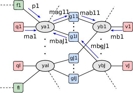
The factorization in (13) provides the basis for a factor graph representation. Contrary to [4], in this work, we consider an alternative factor graph where PO states and association variables are combined in joint variable nodes. In particular, legacy PO states and object-oriented association variables form joint nodes “”. In addition, new PO states and measurement-oriented association variables form joint nodes “”. This combination of variable nodes is motivated by the fact that in the original factor graph there is exactly one connected to the corresponding and exactly one connected to the corresponding . The resulting alternative factor graph leads to a presentation of the proposed method in Section V that is consistent with bp message passing rules [34] as well as the original work on nebp [41]. A single time step of the considered factor graph is shown in Fig. 2a.
Next, bp is applied to efficiently compute the beliefs that approximate the marginal posterior pdf . Since the considered factor graph in Fig. 2a has loops, a specific message-passing order has to be chosen. As in [3, 4], we choose an order that is based on the following rules: (i) BP messages are only sent forward in time, and (ii) iterative message passing is only performed for data association and at each time step individually.
In what follows, we will briefly discuss the calculation of bp messages on the considered factor graph shown in Fig. 2a. Note that messages sent from the singleton factor nodes “” to the joint variable nodes “”, and messages sent from the singleton factor nodes “” to the joint variable nodes “” are equal to the singleton factor nodes “” and “” themselves. Thus, we reuse the same notation for factor nodes and corresponding messages.
IV-1 Prediction Messages
The messages , passed from the factor nodes “” to the joint variable nodes “” are calculated as (cf. [4, Sec. IX-A1])
| (16) |
and where is a scalar that can be computed by making use of and (cf. [4, eq. (77)]). Note the belief and the message are normalized in the sense that they sum to unity,
e.g.,
| (17) |
IV-2 Iterative Probabilistic da
At message passing iteration , the messages and , , passed from variable nodes “” and “” to the indicator nodes “” are given by (cf. (2))
| (18) | ||||
| (19) |
In addition, the messages passed from indicator nodes “” to variables nodes “” and “” are obtained as (cf. (3)),
messages for , and
| (22) | ||||
| (23) |
Here, we have introduced the short notation
| (24) |
and
| (25) |
Note that with a small abuse of notation, one message passing iteration, indexed by , in (22) and (23) corresponds to two message passing iterations in (2) and (3). Iterative message passing (22) and (23) is initialized at , by setting in (23) for all and .
These combined messages can be further simplified [52] as follows. Because of the binary consistency constraints expressed by , each message comprises only two different values. In particular, in (22) takes on one value for and another for all . Furthermore, in (23) takes on one value for and another for all . Thus, each message can be represented (up to an irrelevant constant factor) by the ratio of the first value and the second value, hereafter denoted as for and for . By exchanging simplified messages the computational complexity of each message passing iteration only scales as (see [52, 4] for details). Furthermore, it has been shown in [52] that iterative probabilistic data association following (22)–(23) and its simplified version discussed above are guaranteed to converge.
IV-3 Belief Calculation
Finally, after the last message passing iteration , the beliefs , and , are computed according
to
where , and are normalizing constants that make sure that and sum and integrate to unity. The marginal beliefs , , , and can then be obtained from and by marginalization. In particular, the approximate marginal posterior pdf of augmented states , and , are used for object declaration and state estimation as discussed in Section III-D. Furthermore, the approximate marginal association probabilities , and , are used in a preprocessing step for performance evaluation discussed in Sections VII-A and VII-B.
V Proposed NEBP-based MOT Algorithm
In this section, we start with a discussion on how neural networks can extract features from raw sensor data by using previous state estimates and preprocessed measurements. We then introduce the proposed nebp framework for mot, which compared to bp for MOT uses features as an additional input. Since we limit our discussion to a single time step, we will omit the time index in what
follows.
V-A Feature Extraction
We consider two types of features: (i) features that represent motion information (e.g., position and velocity) and (ii) features that represent shape information.
For each legacy po , the shape feature is extracted
as
| (26) |
where is approximate mmse state estimate of legacy po at the previous time step. Furthermore, is the raw sensor data at the previous time step and is a neural network.
Similarly, for each preprocessed measurement , the shape feature is obtained
as
| (27) |
where is again a neural network and is the raw sensor data collected at the current time step.
Finally, for each legacy po and each measurement , a motion feature is computed according
to
| (28) |
where is the approximate existence probability of legacy po . Furthermore, and are again neural networks. We will discuss one particular instance of shape feature extraction in
Section VII-B.
V-B GNN Topology and BP Message Enhancement
The conjecture of this work is that in many mot applications (i) object dynamics and existence can be described accurately by a statistical model represented by the pdf , and parameters , ; (ii) measurement detection and the resulting measurements of the object’s position can also be described well by a statistical model represented by pdf , and parameters , ; but (iii) object shape information are difficult to represent accurately by a statistical model. Thus, we can make use of models available for (i) and (ii), but for (iii), we best learn the influence of object shape information on measurement detection directly from the data itself. Thus, contrary to the original nebp approach, in our nebp method, only the parts of the mot factor graph that model the data generating process are matched by the gnn. These matched parts are highlighted in Fig. 2. All factor nodes in this part of the factor graph are either singleton or pairwise factor nodes. As discussed in Section II-B, in nebp singleton factor nodes are not matched by gnn nodes. In addition, in our considered factor graph in Fig. 2(a), the pairwise factor nodes “”, and represent simple binary consistency constraints. Thus, we do not explicitly model factor nodes by gnn nodes. The node embeddings of gnn nodes introduced for the variable nodes “”, are denoted as and the node embeddings introduced for variables nodes “”, are denoted as . Finally, following the topology of the factor graph for data association in Fig. 2(a), GNN edges are introduced such that the bipartite GNN shown in Fig. 2(b) is obtained.
We recall from Section II-A that for singleton factor nodes, the message passed to the adjacent variable node is equal to the factor node itself. As a result, and not only describe factor nodes but also the messages that are enhanced. There are two challenges related to directly enhancing these messages based on the GNN according to (5)–(9), i.e., (i) the codomain of and can be very large, which complicates the training of the GNN [53] (see also Sections V-C and VI) and (ii) the messages and involve the continuous random variables and which makes it impossible to enhance them by the output of a gnn for every possible value of and individually.
To address the first challenge, we introduce normalized versions33 3 Multiplying BP messages by a constant factor does not alter the resulting beliefs [34]. of the original BP messages
as
| (29) | ||||
where and
are the normalization constants. Note that after normalization the codomain of and is limited to the interval .
The second challenge is addressed by enhancing bp messages , and , as follows (cf. (9))
| (31) | ||||
| (32) |
Here, and are computed from information provided by the GNN as discussed in the following Section V-C. The other entries of the messages , and , remain unenhanced, i.e., , , , and . Note that calculating nebp messages according to (31) and (32) avoids enhancing and for every possible value of and . All other BP messages are not enhanced.
Finally, neural enhanced data association can be performed by replacing the functions and in (22) and (23) with their neural enhanced counterparts and . These neural enhanced counterparts are obtained by replacing in (24) and (25) the bp messages and with the nebp messages and , respectively. In particular, for we
obtain
| (33) |
and . Similarly, for we
get
| (34) |
and , .
The value , provides a likelihood ratio for the measurement with index being associated to the legacy po with index [4]. In addition, provides a likelihood ratio for the measurement with index being generated by a new po. The shape association term in (33), calculated by the gnn implements object shape association, which can be interpreted as follows. The GNN compares the shape feature extracted for legacy PO with the shape feature extracted for measurement and, if there is a good match, outputs a large . According to (33), this effectively increases the likelihood ratio that the legacy po is associated with the measurement . Note that there is no shape association term in (34). Since the shape feature extracted for new po would be the same as the shape feature for measurement , comparing shape features as performed for legacy POs and measurements is not possible.
The scalar in (33) and (34) provided by the gnn implements false alarm rejection. In particular, is equal to the local increase of the false alarm distribution according to (cf. (29), (), (14), and (15)). In (33), this local increase of the false alarm distribution makes it less likely that the measurement is associated to a legacy PO. In (34), this local increase reduces the existence probability of the new PO introduced for the
measurement .
V-C Statement of the nebp for mot Algorithm
nebp for mot consists of the following steps:
V-C1 Conventional bp
First, the conventional bp-based mot algorithm is run until convergence, from which we obtain , and (cf. Section IV-2), where and .
V-C2 gnn Messages
Next, gnn message passing is
executed iteratively. In particular, at iteration the messages passed along the edges of gnn are computed
as
| (35) | ||||
| (36) |
where is the edge neural network. Furthermore, node embedding vectors of each node are obtained as
| (37) | ||||
| (38) |
where is the node neural network. The iterative processing scheme is initialized by setting node embeddings equal to motion and shape features, i.e., and .
V-C3 NEBP Messages
After computing (35)-(38) for iterations, the refinement used in (31) and (32) is calculated
as
| (39) |
Here, is a neural network and is the sigmoid function. Furthermore, the temperature and the bias are hyperparameters [54] that make it possible to calibrate the transition of the sigmoid.
Finally, the refinement used in (31) is obtained as
| (40) |
where is another neural network and is the rectified linear unit.
V-C4 Belief Calculation
Finally, iterative probabilistic da is again run until convergence by replacing and in (29) and () by its neural enhanced counterparts and in (31) and (32), respectively. This results in the enhanced
messages and (cf. Section IV-2), which are then used for the calculation of legacy po beliefs , and new po beliefs as discussed in Section IV-3.
V-D Complexity Analysis
In this section, we analyze and compare the computational complexity of the conventional bp and the proposed nebp methods for mot. Since both bp and nebp for mot follow the detect-then-track paradigm, the complexity of the detector has to be taken into account. We denote by the number of raw sensor data points. For example, if a LiDAR sensor is considered, this is the number of points of the LiDAR point cloud, and if a camera sensor is used, this is the number of pixels of the camera image. Then the number of operations needed for detection is , where is a constant that depends on the size and type of neural network used as the detector . As discussed in [3, 4], the number of operations needed for the conventional bp method for mot algorithm is , where is a constant that depends on the number of message passing iterations for da, the number of particles, and further parameters. In total, the number of operations for bp is . Thus, the computational complexity of bp scales as .
The additional operations of nebp compared to conventional bp are related to feature extraction and the gnn. Feature extraction as discussed in (26)–(28) requires operations, where are constants that depend on the size and type of the neural networks , respectively. The gnn is a fully connected bipartite graph, i.e., it consists of two sets of nodes, and each node in the first set is connected via an edge to each node in the second set. The number of nodes in each set is equal to and , respectively. GNN messages are exchanged on the edges of the network according to (35) and (36). This is followed by GNN messages aggregation in (37) and (38), as well as BP message refinement in (39) and (40). The total number of operations is hence equal to , where depends on the size and type of neural networks , , , and . It can thus be seen, that the computational complexity of nebp also scales as . Note that due to the additional operations performed by nebp, the runtime of nebp is longer compared to bp. Runtimes of bp and nebp are further analyzed in Section VII-D.
VI Loss Function and Training
Training of the proposed nebp method is performed in a supervised manner. It is assumed that a training set consisting of ground truth object tracks is available. A ground truth object track is a sequence of object positions. Every sequence is characterized by an object identity (ID). During the training phase, the parameters of all neural networks are updated through back-propagation, which computes the gradient of the loss function. The loss function has the form , where the two contributions and are related to false alarm rejection and object shape association, respectively.
Thus, we consider the following binary cross-entropy loss [55, Chapter 4.3] for false alarm rejection, i.e.,
| (41) |
where is the pseudo ground truth label for each measurement and is a tuning parameter. The pseudo ground truth label is equal to if the distance between the measurement and any ground truth position is smaller or equal to , and otherwise. The tuning parameter addresses the imbalance problem in learning-based binary classification (see [56] for details). This problem is caused by the fact that, since missing an object is typically more severe than producing a false alarm, object detectors produce more false alarm measurements than true measurements.
Since in (33) represents the likelihood that the legacy po is associated to the measurement , ideally is large if po is associated to the measurement , and is equal to zero if they are not associated. Thus, we consider the following binary cross-entropy loss for object shape association,
i.e.,
| (42) |
where is the sigmoid function and is the pseudo ground truth association vector of legacy po . In each pseudo ground truth association vector , at most one element is equal to one and all the other elements are equal to zero. We apply instead of in the binary entropy loss (42). This is because the otherwise ReLU operation “blocks” certain gradients, i.e., gradients are zero for negative values of . It was been observed, that by performing backpropagation by also making use of the gradients related to the negative values of , the gnn can be trained more efficiently.
At each time step, pseudo ground truth association vectors are constructed from measurements and ground truth object tracks based on the following
rules:
- •
Get Measurement IDs: First, the Euclidean distance between all ground truth positions and measurements is computed. Next, the Hungarian algorithm [1] is performed to find the best association between ground truth positions and measurements. Finally, all measurements that have been associated with a ground truth position and have a distance to that ground truth position that is smaller than , inherit the ID of the ground truth position. All other measurements do not have an ID.
- •
Update Legacy PO IDs: Legacy POs inherit the ID from the previous time step. If a legacy PO with ID has a distance not larger than to a ground truth position with the same ID, it keeps its ID. If a legacy PO has the same ID as measurement , the entry is set to one. All other entries , , are set to zero.
- •
Introduce New PO IDs: A new PO inherits the ID from the corresponding measurement if the measurement has an ID that is different from the ID of any legacy po. All other new POs do not have an
ID.
VII Numerical Results
To validate the performance of our method, we present results in an autonomous driving
scenario.
VII-A Experimental Setup
VII-A1 Dataset
Our numerical evaluation is based on the nuScenes autonomous driving dataset [57], which contains 1000 autonomous driving scenes. We use the official predefined dataset split, where 700 scenes are considered for training, 150 for validation, and 150 for testing. Each scene has a length of roughly 20 seconds and contains keyframes (frames with ground truth annotations) sampled at 2Hz. There are seven object classes. The proposed mot method and reference techniques are performed for each class individually. If not stated otherwise, all the operations described next are performed for each class separately. In this paper, we only consider LiDAR data provided by the nuScenes dataset. A scene of the considered autonomous driving application is shown in Fig. 3.
VII-A2 System Model
The state of a po consists of its 2-D position and 2-D velocity. Preprocessed measurements are extracted from the LiDAR data. For the extraction of preprocessed measurements, we employed the CenterPoint [13] detector which is based on deep learning44 4 The measurements provided by the CenterPoint detector are further preprocessed using nms (nms) with 3-D iou [58, 19] where the threshold is set to 0.1. . Any preprocessed measurement consists of 2-D position, 2-D velocity, and a confidence score .
Object dynamics are modeled by a constant-velocity motion model [59]. Object tracking is performed in a global reference frame that is predefined for each scene [57]. The considered roi (roi) is defined by , where is the 2-D position of the “ego vehicle” that is equipped with the LiDAR sensor. The pdf that describe false alarms and unknown objects are uniformly distributed over the roi. The measurement model that defines the likelihood function is linear with additive Gaussian noise, i.e., , where with being the diagonal covariance matrix. The probability of survival is set to . The threshold for target declaration is .
The pruning threshold discussed in Section III-D is set to . In addition, we also prune new POs with to further reduce the number of false objects and computational complexity. All other parameters used in the system model are extracted from training data. For the bp part of the proposed nebp method, we use the particle-based implementation introduced in [3].
VII-A3 Performance Metrics
We consider using the amota (amota) metric proposed in [16] to evaluate the performance of our algorithm. In addition, we also use the widely used CLEAR metrics [60] and track quality measures [61] that include the number of ids (ids) and track frag (frag). The number of ids is increased if a ground truth object is matched to an estimated object with index at the current time step, while it was matched to an estimated object with index at a previous time. The number of frag is increased if a ground truth object is matched to an estimated object at the previous time step, but it is not matched to any estimated objects at the current time step. Note that amota is the primary metric used by the nuScenes tracking challenge
[57].
VII-B Implementation Details
For shape features extraction as discussed in Section V-A, a neural network that consists of two stages is introduced. The first stage is a VoxelNet [24], a neural network architecture that is used as the backbone for a variety of object detectors [13, 26]. The VoxelNet takes the LiDAR scan as input, and outputs a 3D tensor of size . This tensor is typically referred to as feature map. The first two dimensions of the feature map form a grid with elements that cover the roi. For each grid point, there is a feature vector with elements. The second stage is a cnn (cnn) that consists of two convolutional layers and a single-hidden-layer mlp (mlp). Here, we use a cnn since it has fewer trainable parameters compared to an MLP and is thus easier to train. Note that cnn have been widely used for feature extraction [62, 24]. The cnn extracts shape features from a reduced feature map, as discussed next.
For the extraction of shape features in the second stage, at first, the grid point of the feature map that corresponds to the considered po or measurements is located. Then, the feature vector at this grid point and the 8 feature vectors at adjacent grid points are extracted. As a result, for each po and each measurement, a reduced feature map of size is extracted. This reduced feature map is then used as the input of a cnn. Finally, the cnn computes the shape feature or . The considered feature map of dimension has been precomputed by the CenterPoint [13] method. The same VoxelNet is shared across all seven object classes. Its parameters remain fixed during the training of the proposed method.
The other neural networks , , , , and are mlp with a single hidden layer and a leaky ReLU activation function. All feature vectors, i.e., and , as well as and , , consist of 128 elements. The number of gnn iterations is . Training of the proposed method is performed based on the Adam optimizer [63]. The batch size, learning rate, and the number of “epochs”, i.e., the number of times the Adam optimizer processes the entire training dataset, are set to , , and , respectively. The hyperparameter in (41) is set to 0.1 and the threshold for the pseudo ground truth extraction discussed in Section VI is
set to 2 meters.
Evaluation of amota requires a score for each estimated object. It was observed that a high amota performance is obtained by calculating the estimated object score as a combination of existence probability and measurement score. In particular, for legacy po we calculate an estimated object score
as
| (43) |
For new PO the estimated object score is given by
.
VII-C Calibration
The calibration of the sigmoid introduced in (39) is performed as follows. For training, we set and . However, for inference we set and such that the sigmoid in (39) transitions to one quicker and for smaller values of . The different calibration values for inference are necessary because the loss function used for training and the AMOTA metric used for performance evaluation behave differently. In particular, for performance evaluation based on AMOTA, missing an object is significantly more severe than a false object. (Note that the AMOTA metric can not directly be used for training because it is not differentiable [55].) The calibration values and used for inference are selected based on a grid search over possible values and . The values for and that achieved the highest amota value on a subset of the training set were obtained as and for the classes bicycle, bus, car, motorcycle, pedestrian, trailer, and truck, respectively.
VII-D Performance Evaluation
For performance evaluation, we use state-of-the-art reference methods that all use measurements provided by the CenterPoint detector [13], which was the best LiDAR-only object detector for the nuScenes dataset at the time of the submission of this paper. In particular, bp refers to the conventional bp-based mot method [4]. CenterPointT refers to the tracking method proposed in [13]. It uses a heuristic to create new tracks and a greedy matching algorithm based on the Euclidean distance to associate measurements provided by the CenterPoint detector. The methods in [64, 22, 19] all follow a similar strategy. The CBMOT method [64] adopts a score update function for estimated object scores. Chiu et al. [22] make use of a hybrid distance that combines the Mahalanobis distance with a proposed deep feature distance. SimpleTrack [19] uses the giou (giou) as the distance for measurement association. In SimpleTrack [19], the object detector is also applied to non-keyframes and has a measurement rate of 10Hz. The Immortal tracker [20] has a measurement rate of 2Hz. It follows the tracking approach of SimpleTrack, except that it never terminates tracks. PMB [11] implements a Poisson multi-Bernoulli filter for mot that relies on a global nearest neighbor approach for data association. Finally, OGR3MOT [17] utilizes a network flow formulation and transforms the data association problem into a classification problem.
| Method | Modalities | AMOTA | IDS | Frag |
|---|---|---|---|---|
| CenterPointT [13] | LiDAR | 0.638 | 760 | 529 |
| CBMOT [64] | LiDAR | 0.649 | 557 | 450 |
| Chiu et al. [22] | LiDAR+Camera | 0.655 | 1043 | 717 |
| OGR3MOT [17] | LiDAR | 0.656 | 288 | 371 |
| SimpleTrack [19] | LiDAR | 0.668 | 575 | 591 |
| Immortal [20] | LiDAR | 0.677 | 320 | 477 |
| PMB [11] | LiDAR | 0.678 | 770 | 431 |
| BP | LiDAR | 0.666 | 182 | 245 |
| NEBP (proposed) | LiDAR | 0.683 | 227 | 299 |
| Method | Modalities | AMOTA | IDS | Frag |
|---|---|---|---|---|
| CenterPointT [13] | LiDAR | 0.665 | 562 | 424 |
| CBMOT [64] | LiDAR | 0.675 | 494 | - |
| Chiu et al. [22] | LiDAR+Camera | 0.687 | - | - |
| OGR3MOT [17] | LiDAR | 0.693 | 262 | 332 |
| SimpleTrack [19] | LiDAR | 0.696 | 405 | - |
| Immortal [20] | LiDAR | 0.702 | 385 | - |
| PMB [11] | LiDAR | 0.707 | 650 | 345 |
| BP | LiDAR | 0.698 | 161 | 250 |
| NEBP (proposed) | LiDAR | 0.708 | 172 | 271 |


| Detector | Method | AMOTA | IDS | Frag |
|---|---|---|---|---|
| PointPillar [25] | BP | 0.360 | 226 | 658 |
| NEBP (proposed) | 0.398 | 270 | 418 | |
| Megvii [26] | BP | 0.637 | 108 | 262 |
| NEBP (proposed) | 0.651 | 136 | 252 | |
| CenterPoint [13] | BP | 0.698 | 161 | 250 |
| NEBP (proposed) | 0.708 | 172 | 271 |
In Table I and II, we present the tracking performance of the considered methods on the nuScenes validation and test sets based on measurements provided by the CenterPoint detector. The symbol “-” in Table II indicates that the metric is not reported. It can be seen that the proposed nebp approach outperforms all reference methods in terms of amota performance. Furthermore, it can be observed, that bp and nebp achieve a much lower ids and frag metric compared to the reference methods. This is because both bp and nebp make use of a statistical model to determine the initialization and termination of tracks [4], which is more robust compared to the heuristic track management performed by other reference methods. The improved amota performance of nebp over bp comes at the cost of a slightly increased ids and frag. Qualitative results for a single time step of an example autonomous driving scene are shown in Fig. 4. It can be seen that compared to CenterPointT, bp can reduce the number of false objects significantly, while nebp can reduce the number of false alarms even further. We also report estimation performance results based on the gospa (gospa) metric [65]. This metric can be split up into three components, namely, localization error, false estimated objects, and missed ground truth objects. nebp outperforms bp in all three components.
| Method | GOSPA | Localization | False | Missed |
|---|---|---|---|---|
| BP | 1.163 | 0.327 | 0.127 | 0.709 |
| NEBP (proposed) | 1.140 | 0.318 | 0.123 | 0.699 |
We also compare the performance of the proposed NEBP method with BP based on measurements provided by different object detectors. In particular, in addition to measurements provided by the CenterPoint [13] detector, we also consider measurements provided by the PointPillar [25] and the Megvii [26] detectors. Results based on the nuScenes validation set are shown in Table III. For all three detectors, nebp can outperform bp in terms of amota, and at the same time maintain a similar number of ids and frag. These results indicated that the proposed nebp method is robust with respect to the chosen object detector.
All experiments were executed on a single Nvidia P100 GPU. For training, eight epochs of the nuScenes training set were performed. The total training time was measured as 30 hours. The inference times of bp and nebp applied to the nuScenes validation were measured as 658 seconds and 1137 seconds. These times do not include the execution of the object detector, which yields a runtime of 822 seconds. nebp has a higher computational complexity compared to bp due to the additional operations discussed in Section V-D.
VII-E Ablation Study
In this section, we analyze the contribution of different algorithmic components to the overall performance of our nebp method. In particular, we analyze the degradations of nebp performance that are the result of the ablation of specific algorithmic components. All ablation studies are based on the nuScenes validation set, and measurements provided by the CenterPoint detector [13].
We aim to quantify the performance benefits of nebp resulting from using shape features as an additional input. We consider three nebp variants: “NEBP-m”, “NEBP-r” and “NEBP-a”. NEBP-m does not make use of shape features. In particular, it initializes the gnn node embeddings only based on motion features, i.e., and . The two variants NEBP-r and NEBP-a are introduced to quantify the benefits of false alarm rejection and object shape association, respectively. More specifically, NEBP-r focuses on false alarm rejection only, i.e., in (31) object shape association is deactivated by setting . Similarly, NEBP-a focuses on object shape association only, i.e., in (31) and (32) false alarm rejection is deactivated by setting .
| Method | AMOTA | IDS | Frag |
|---|---|---|---|
| BP | 0.698 | 161 | 250 |
| NEBP-m | 0.698 | 183 | 228 |
| NEBP-a | 0.703 | 195 | 259 |
| NEBP-r | 0.706 | 178 | 227 |
| NEBP-nc | 0.703 | 180 | 250 |
| NEBP (proposed) | 0.708 | 172 | 271 |
Table V shows the tracking performance of these nebp variants, conventional bp, and the proposed nebp method. It can be seen that NEBP-m can not achieve any performance improvements compared to bp. This is not surprising since object motion is already modeled accurately by the statistical model and, compared to bp, NEBP-m does not make use of any additional information. On the other hand, both NEBP-a and NEBP-r can achieve an improved amota performance compared to bp. This is because NEBP-a and NEBP-r incorporate additional information in the form of shape features and address the fact that the statistical model used by bp does not accurately model the true data-generating process. In particular, in the statistical model, false alarm measurements are uniformly distributed over the roi. Furthermore, false alarm measurement and their number are also assumed to be independent and identically distributed across time. However, these assumptions do often not hold in real-world mot applications such as the considered autonomous driving scenario. This is because physical structures and other reflecting features in the environment can generate so-called persistent false alarm measurements. These false alarm measurements are not uniformly distributed and are not independent across time. Thus, they are not accurately represented by the considered statistical model. This model mismatch degrades tracking performance and is addressed by false alarm rejection performed by NEBP and NEBP-r. Object shape association as performed by NEBP and NEBP-a improves data association by using object shape information provided by shape features.
Finally, Table V also reports performance improvements that result from the calibration process discussed in Section VII-C. In particular, “NEBP-nc” is the NEBP variant where no calibration has been performed, i.e., we have and for training and inference. It can be seen that calibration can significantly improve the performance of nebp.
The effect of temperature parameters for five representative object classes is shown in Table VI. For each class, the bias is fixed to the value provided above. Note that , is equivalent to discarding all measurements with . It can be seen that nebp does not always achieve the best amota for . In cases where it is difficult to determine whether a measurement is a false alarm, using a temperature can be more robust, as it does not directly discard the measurements with , but instead reduces the estimated object score (43) of po that are likely to generate these
measurements.
| Temperature | bicycle | pedestrian | motorcycle | trailer | truck |
|---|---|---|---|---|---|
| 0.528 | 0.807 | 0.737 | 0.568 | 0.662 | |
| 0.534 | 0.809 | 0.727 | 0.565 | 0.663 | |
| 0.527 | 0.810 | 0.716 | 0.563 | 0.662 | |
| 0.550 | 0.815 | 0.727 | 0.566 | 0.664 | |
| 0.544 | 0.814 | 0.739 | 0.569 | 0.662 | |
| 0.540 | 0.813 | 0.730 | 0.562 | 0.662 | |
| 0.547 | 0.814 | 0.736 | 0.567 | 0.657 | |
| 0.550 | 0.813 | 0.739 | 0.559 | 0.656 |
VIII Conclusion
In this paper, we present a nebp method for mot that enhances the solution of model-based bp by making use of shape features learned from raw sensor data. Our approach conjectures that learned information can reduce model mismatch and thus improve data association and rejection of false alarms. A gnn that matches the topology of the factor graph used for model-based data association is introduced. For false alarm rejection, the gnn identifies measurements that are likely false alarms. For object shape association, the gnn computes corrections terms that result in more accurate association probabilities. The proposed approach can improve the object declaration and state estimation performance of bp while preserving its favorable scalability of the computational complexity. Furthermore, the proposed nebp method inherits the robust track management of bp-based algorithms. We employed the nuScenes autonomous driving dataset for performance evaluation and demonstrated state-of-the-art object tracking performance. Due to robust track management nebp yields a much lower number of ids and track frag compared to non-bp-based reference
methods. A promising direction for future research is an application of the proposed nebp approach to multipath-aided localization
[66].
.
References
- [1] Y. Bar-Shalom, P. K. Willett, and X. Tian, Tracking and Data Fusion: A Handbook of Algorithms. Storrs, CT: Yaakov Bar-Shalom, 2011.
- [2] R. Mahler, Statistical Multisource-Multitarget Information Fusion. Norwood, MA: Artech House, 2007.
- [3] F. Meyer, P. Braca, P. Willett, and F. Hlawatsch, “A scalable algorithm for tracking an unknown number of targets using multiple sensors,” IEEE Trans. Signal Process., vol. 65, no. 13, pp. 3478–3493, Jul. 2017.
- [4] F. Meyer, T. Kropfreiter, J. L. Williams, R. A. Lau, F. Hlawatsch, P. Braca, and M. Z. Win, “Message passing algorithms for scalable multitarget tracking,” Proc. IEEE, vol. 106, no. 2, pp. 221–259, Feb. 2018.
- [5] F. Meyer and J. L. Williams, “Scalable detection and tracking of geometric extended objects,” IEEE Trans. Signal Process., vol. 69, pp. 6283–6298, 2021.
- [6] J. L. Williams, “Marginal multi-Bernoulli filters: RFS derivation of MHT, JIPDA and association-based MeMBer,” IEEE Trans. Aerosp. Electron. Syst., vol. 51, no. 3, pp. 1664–1687, Jul. 2015.
- [7] Á. F. García-Fernández, J. L. Williams, K. Granström, and L. Svensson, “Poisson multi-Bernoulli mixture filter: Direct derivation and implementation,” IEEE Trans. Aerosp. Electron. Syst., vol. 54, no. 4, pp. 1883–1901, Feb. 2018.
- [8] S. Scheidegger, J. Benjaminsson, E. Rosenberg, A. Krishnan, and K. Granström, “Mono-camera 3D multi-object tracking using deep learning detections and PMBM filtering,” in Proc. IEEE IV-18, Jun. 2018, pp. 433–440.
- [9] G. Soldi, F. Meyer, P. Braca, and F. Hlawatsch, “Self-tuning algorithms for multisensor-multitarget tracking using belief propagation,” IEEE Trans. Signal Process., vol. 67, no. 15, pp. 3922–3937, Aug. 2019.
- [10] S. Pang, D. Morris, and H. Radha, “3D multi-object tracking using random finite set-based multiple measurement models filtering (RFS-M3) for autonomous vehicles,” in Proc. ICRA-21, Jun. 2021, pp. 13 701–13 707.
- [11] J. Liu, L. Bai, Y. Xia, T. Huang, and B. Zhu, “GNN-PMB: A simple but effective online 3D multi-object tracker without bells and whistles,” arXiv preprint arxiv.2206.10255, 2022.
- [12] W. Zhang and F. Meyer, “Graph-based multiobject tracking with embedded particle flow,” in Proc. IEEE RadarConf-21, May 2021, pp. 1–6.
- [13] T. Yin, X. Zhou, and P. Krahenbuhl, “Center-based 3D object detection and tracking,” in Proc. CVPR-21, Jun. 2021, pp. 11 784–11 793.
- [14] F. Meyer and M. Z. Win, “Scalable data association for extended object tracking,” IEEE Trans. Signal Inf. Process. Netw., vol. 6, pp. 491–507, May 2020.
- [15] H.-k. Chiu, A. Prioletti, J. Li, and J. Bohg, “Probabilistic 3D multi-object tracking for autonomous driving,” arXiv preprint arXiv:2001.05673, 2020.
- [16] X. Weng, J. Wang, D. Held, and K. Kitani, “3D multi-object tracking: A baseline and new evaluation metrics,” in Proc. IROS-20, Oct. 2020, pp. 10 359–10 366.
- [17] J.-N. Zaech, D. Dai, A. Liniger, M. Danelljan, and L. Van Gool, “Learnable online graph representations for 3D multi-object tracking,” IEEE Robot. Autom. Lett., vol. 7, no. 2, pp. 5103–5110, Jan. 2022.
- [18] A. Rangesh, P. Maheshwari, M. Gebre, S. Mhatre, V. Ramezani, and M. M. Trivedi, “TrackMPNN: A message passing graph neural architecture for multi-object tracking,” arXiv preprint arXiv:2101.04206, 2021.
- [19] Z. Pang, Z. Li, and N. Wang, “SimpleTrack: Understanding and rethinking 3D multi-object tracking,” arXiv preprint arXiv:2111.09621, 2021.
- [20] Q. Wang, Y. Chen, Z. Pang, N. Wang, and Z. Zhang, “Immortal Tracker: Tracklet never dies,” arXiv preprint arXiv:2111.13672, 2021.
- [21] X. Weng, Y. Wang, Y. Man, and K. M. Kitani, “GNN3DMOT: Graph neural network for 3D multi-object tracking with 2D-3D multi-feature learning,” in Proc. CVPR-20, Jun. 2020, pp. 6499–6508.
- [22] H.-k. Chiu, J. Li, R. Ambrus, and J. Bohg, “Probabilistic 3D multi-modal, multi-object tracking for autonomous driving,” in Proc. ICRA-21, Jun. 2021, pp. 14 227–14 233.
- [23] X. Li, E. Leitinger, A. Venus, and F. Tufvesson, “Sequential detection and estimation of multipath channel parameters using belief propagation,” IEEE Trans. Wireless Commun., vol. 21, no. 10, pp. 8385–8402, 2022.
- [24] Y. Zhou and O. Tuzel, “Voxelnet: End-to-end learning for point cloud based 3D object detection,” in Proc. CVPR-18, Jun. 2018, pp. 4490–4499.
- [25] A. H. Lang, S. Vora, H. Caesar, L. Zhou, J. Yang, and O. Beijbom, “PointPillars: Fast encoders for object detection from point clouds,” in Proc. CVPR-19, Jun. 2019, pp. 12 697–12 705.
- [26] B. Zhu, Z. Jiang, X. Zhou, Z. Li, and G. Yu, “Class-balanced grouping and sampling for point cloud 3D object detection,” arXiv:1908.09492, 2019.
- [27] S. Ren, K. He, R. Girshick, and J. Sun, “Faster R-CNN: Towards real-time object detection with region proposal networks,” in Proc. NeurIPS-15, vol. 28, Dec. 2015, pp. 91–99.
- [28] S. Shi, X. Wang, and H. Li, “PointRCNN: 3D object proposal generation and detection from point cloud,” in Proc. CVPR-19, Jun. 2019, pp. 770–779.
- [29] A. Simonelli, S. R. Bulo, L. Porzi, M. López-Antequera, and P. Kontschieder, “Disentangling monocular 3D object detection,” in Proc. CVPR-19, Jun. 2019, pp. 1991–1999.
- [30] K. Okuma, A. Taleghani, N. d. Freitas, J. J. Little, and D. G. Lowe, “A boosted particle filter: Multitarget detection and tracking,” in Proc. ECCV-04, 2004, pp. 28–39.
- [31] M. D. Breitenstein, F. Reichlin, B. Leibe, E. Koller-Meier, and L. Van Gool, “Online multiperson tracking-by-detection from a single, uncalibrated camera,” IEEE Trans. Pattern Anal. Mach. Intell., vol. 33, no. 9, pp. 1820–1833, 2010.
- [32] H. W. Kuhn, “The Hungarian method for the assignment problem,” NRL quarterly, vol. 2, no. 1-2, pp. 83–97, Mar. 1955.
- [33] S. S. Blackman, “Multiple hypothesis tracking for multiple target tracking,” IEEE Trans. Aerosp. Electron. Syst., vol. 19, pp. 5–18, Jan. 2004.
- [34] F. R. Kschischang, B. J. Frey, and H.-A. Loeliger, “Factor graphs and the sum-product algorithm,” IEEE Trans. Inf. Theory, vol. 47, no. 2, pp. 498–519, Feb. 2001.
- [35] J. Yedidia, W. Freemand, and Y. Weiss, “Constructing free-energy approximations and generalized belief propagation algorithms,” IEEE Trans. Inf. Theory, vol. 51, no. 7, pp. 2282–2312, July 2005.
- [36] D. Koller and N. Friedman, Probabilistic Graphical Models: Principles and Techniques. Cambridge, MA: MIT Press, 2009.
- [37] M. S. Arulampalam, S. Maskell, N. Gordon, and T. Clapp, “A tutorial on particle filters for online nonlinear/non-Gaussian Bayesian tracking,” IEEE Trans. Signal Process., vol. 50, no. 2, pp. 174–188, Feb. 2002.
- [38] M. Gori, G. Monfardini, and F. Scarselli, “A new model for learning in graph domains,” in Proc. INNS/IEEE IJCNN-05, vol. 2, Aug. 2005, pp. 729–734.
- [39] J. Gilmer, S. S. Schoenholz, P. F. Riley, O. Vinyals, and G. E. Dahl, “Neural message passing for quantum chemistry,” in Proc. ICML-17, Aug. 2017, pp. 1263–1272.
- [40] K. Yoon, R. Liao, Y. Xiong, L. Zhang, E. Fetaya, R. Urtasun, R. Zemel, and X. Pitkow, “Inference in probabilistic graphical models by graph neural networks,” in Proc. IEEE Asilomar-19, 2019, pp. 868–875.
- [41] V. G. Satorras and M. Welling, “Neural enhanced belief propagation on factor graphs,” in Proc. AISTATS-21, Apr. 2021, pp. 685–693.
- [42] M. Liang and F. Meyer, “Neural enhanced belief propagation for cooperative localization,” in Proc. IEEE SSP-21, Jul. 2021, pp. 326–330.
- [43] K. Granström, M. Baum, and S. Reuter, “Extended object tracking: Introduction, overview and applications,” J. Adv. Inf. Fusion, vol. 12, no. 2, pp. 139–174, Dec. 2017.
- [44] K. Granström, M. Fatemi, and L. Svensson, “Poisson multi-Bernoulli mixture conjugate prior for multiple extended target filtering,” IEEE Trans. Aerosp. Electron. Syst., vol. 56, no. 1, pp. 208–225, Feb. 2020.
- [45] M. Liang and F. Meyer, “Neural enhanced belief propagation for data association in multiobject tracking,” in Proc. FUSION-22, Jul. 2022.
- [46] H.-A. Loeliger, “An introduction to factor graphs,” IEEE Signal Process. Mag., vol. 21, no. 1, pp. 28–41, 2004.
- [47] H. Wymeersch, Iterative Receiver Design. Cambridge University Press, 2007.
- [48] M. J. Wainwright and M. I. Jordan, “Graphical models, exponential families, and variational inference,” University of California, Berkeley, Tech. Rep. TR-649, Sep. 2003.
- [49] M. Bayati, D. Shah, and M. Sharma, “Max-product for maximum weight matching: Convergence, correctness, and LP duality,” IEEE Trans. Inf. Theory, vol. 54, no. 3, pp. 1241–1251, 2008.
- [50] J. L. Williams and R. A. Lau, “Data association by loopy belief propagation,” in Proc. FUSION-10, 2010, pp. 1–8.
- [51] H. V. Poor, An Introduction to Signal Detection and Estimation, 2nd ed. New York: Springer-Verlag, 1994.
- [52] J. L. Williams and R. Lau, “Approximate evaluation of marginal association probabilities with belief propagation,” IEEE Trans. Aerosp. Electron. Syst., vol. 50, no. 4, pp. 2942–2959, Oct. 2014.
- [53] S. Ioffe and C. Szegedy, “Batch normalization: Accelerating deep network training by reducing internal covariate shift,” in Proc. ICML-15, Jul. 2015, pp. 448–456.
- [54] C. Guo, G. Pleiss, Y. Sun, and K. Q. Weinberger, “On calibration of modern neural networks,” in Proc. ICML-17, Aug. 2017, pp. 1321–1330.
- [55] C. M. Bishop, Pattern Recognition and Machine Learning (Information Science and Statistics). Berlin, Heidelberg: Springer-Verlag, 2006.
- [56] K. Oksuz, B. C. Cam, S. Kalkan, and E. Akbas, “Imbalance problems in object detection: A review,” IEEE Trans. Pattern Anal. Mach. Intell., vol. 43, no. 10, pp. 3388–3415, Mar. 2020.
- [57] H. Caesar, V. Bankiti, A. H. Lang, S. Vora, V. E. Liong, Q. Xu, A. Krishnan, Y. Pan, G. Baldan, and O. Beijbom, “nuScenes: A multimodal dataset for autonomous driving,” in Proc. CVPR-20, Jun. 2020, pp. 11 621–11 631.
- [58] A. Neubeck and L. Van Gool, “Efficient non-maximum suppression,” in Proc. ICPR-06, vol. 3, Aug. 2006, pp. 850–855.
- [59] Y. Bar-Shalom, T. Kirubarajan, and X.-R. Li, Estimation with Applications to Tracking and Navigation. New York, NY: Wiley, 2002.
- [60] K. Bernardin and R. Stiefelhagen, “Evaluating multiple object tracking performance: the CLEAR MOT metrics,” EURASIP J. Image Video Proc., vol. 2008, pp. 1–10, May 2008.
- [61] B. Wu and R. Nevatia, “Tracking of multiple, partially occluded humans based on static body part detection,” in Proc. of CVPR-06, vol. 1, Jun. 2006, pp. 951–958.
- [62] Y. LeCun, B. Boser, J. Denker, D. Henderson, R. Howard, W. Hubbard, and L. Jackel, “Handwritten digit recognition with a back-propagation network,” in Proc. NeurIPS-89, vol. 2, Nov. 1989, pp. 396–404.
- [63] D. P. Kingma and J. Ba, “Adam: A method for stochastic optimization,” arXiv preprint arXiv:1412.6980, 2014.
- [64] N. Benbarka, J. Schröder, and A. Zell, “Score refinement for confidence-based 3D multi-object tracking,” in Proc. IROS-21, Sep. 2021, pp. 8083–8090.
- [65] A. S. Rahmathullah, Á. F. García-Fernández, and L. Svensson, “Generalized optimal sub-pattern assignment metric,” in Proc. FUSION-17, Jul. 2017, pp. 1–8.
- [66] E. Leitinger, F. Meyer, F. Hlawatsch, K. Witrisal, F. Tufvesson, and M. Z. Win, “A scalable belief propagation algorithm for radio signal based SLAM,” IEEE Trans. Wireless Commun., vol. 18, no. 12, Dec. 2019.