ReCo: Reliable Causal Chain Reasoning via Structural Causal Recurrent Neural Networks
Abstract
Causal chain reasoning (CCR) is an essential ability for many decision-making AI systems, which requires the model to build reliable causal chains by connecting causal pairs. However, CCR suffers from two main transitive problems: threshold effect and scene drift. In other words, the causal pairs to be spliced may have a conflicting threshold boundary or scenario. To address these issues, we propose a novel Reliable Causal chain reasoning framework (ReCo), which introduces exogenous variables to represent the threshold and scene factors of each causal pair within the causal chain, and estimates the threshold and scene contradictions across exogenous variables via structural causal recurrent neural networks (SRNN). Experiments show that ReCo outperforms a series of strong baselines on both Chinese and English CCR datasets. Moreover, by injecting reliable causal chain knowledge distilled by ReCo, BERT can achieve better performances on four downstream causal-related tasks than BERT models enhanced by other kinds of knowledge.
1 Introduction
Causal chain reasoning aims at understanding the long-distance causal dependencies of events and building reliable causal chains. Here, reliable means that events in the causal chain can naturally occur in the order of causal evolution within some circumstance based on the commonsense Roemmele et al. 2011. Causal chain knowledge is of great importance for various artificial intelligence applications, such as question answering Asai et al. 2019, and abductive reasoning Du et al. 2021a. Many studies focus on the reliability of causal pair knowledge but ignore that of causal chain knowledge, especially in the natural language processing (NLP) community.
Previous works mainly acquire causal chain knowledge by first extracting precise causal pairs from text with rule-based Heindorf et al. 2020; Li et al. 2020 or neural-based Ding et al. 2019; Zhang et al. 2020 methods, then connecting these causal pairs into causal chains based on the textual or semantic similarity between events. However, this straightforward approach may bring some transitive problems Johnson and Ahn 2015, leading to unreliable causal chains, which would hinder causal-enhanced models to get higher performances. For example, given a cause event: “playing basketball”, and two candidate effect events: “gets a technical foul” and “gets a red card”, an unreliable causal chain (“playing basketball”“dispute”“gets a red card”) would mislead the model to choose the less plausible effect “gets a red card”.
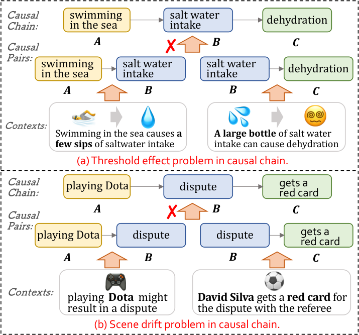
Among these transitive problems Johnson and Ahn 2015, threshold effect and scene drift are the most two salient ones. As shown in Figure 1 (a), given two causal pairs (A causes B, and B causes C), the threshold effect problem is that the influence of A on B is not enough for B to cause C. We can notice that, “swimming in the sea” can only result in tens of milliliters of “salt water intake”, while “dehydration” is caused by hundreds of milliliters of “salt water intake”. Therefore, “salt water intake” conditioned on “swimming in the sea” cannot lead to “dehydration”. Similarly, as shown in Figure 1 (b), the scene drift problem means that A B and B C would not happen within the same specific scene. These two “dispute” events are wrongly joined together by their surface forms. “Dispute” that happened in a video game scene cannot lead to “gets a red card” in a football match scene. Therefore, we find that the threshold effect and scene drift problems are caused by the contradictions between the threshold factors and between the scene factors, respectively.
To address these two issues, in ReCo, we first build a structural causal model (SCM) Pearl 2009 for each causal chain, and the SCM introduces exogenous variables to represent the threshold and scene factors of the causal pairs within the causal chain. Then, we conduct an exogenous-aware conditional variational autoencoder (EA-CVAE) to implicitly learn the semantic representations of exogenous variables according to the contexts of the causal pairs. Subsequently, we devise a novel causal recurrent neural network named SRNN to estimate the contradictions between the exogenous variables by modeling the semantic distance between them. Finally, we present a task-specific logic loss to better optimize ReCo.
Extensive experiments show that our method outperforms a series of baselines on both Chinese and English CCR datasets. The comparative experiments on different lengths of the causal chains further illustrate the superiority of our method. Moreover, BERT Devlin et al. 2019 injected with reliable casual chains distilled by ReCo, achieves better results on four downstream causal-related tasks, which indicates that ReCo could provide more effective and reliable causal knowledge. The code is available on https://github.com/Waste-Wood/ReCo.

2 Background
2.1 Problem Definition
In this paper, the CCR task is defined as a binary classification problem. Specifically, input a reliable antecedent causal chain () and a causal pair (), the model needs to output whether the causal chain is reliable or not.
2.2 Structural Causal Model
Structural Causal Model (SCM) was proposed by Pearl 2009, which is a probabilistic graph model that represents causality within a single system. SCM is defined as an ordered triple , where is a set of exogenous variables determined by external (implicit) factors of the system. is a set of endogenous variables determined by internal (explicit) factors of the system. is a set of structural equations, each structural equation represents the probability of an endogenous variable with the variables in and .

As shown in Figure 2 (a), given two causal pairs ( and ), they can be connected into a causal chain (). We construct an SCM for this causal chain. Events ( and ) are the endogenous variables, and exogenous variables (, ) contain the threshold and scene factors of the causal pairs. Each structural equation represents the probability of an endogenous variable in (eg. (|)). And as shown in Figure 2 (b), if the causal chain possesses threshold effect or scene drift problem, there are contradictions between and .
3 Method
3.1 Overview
In this paper, we devise ReCo to estimate the reliability of the input causal chain. Figure 3 (a) shows the architecture of ReCo, which consists of four components: (1) an encoder to encode causal events and their contexts into dense vectors; (2) an exogenous-aware CVAE to capture the exogenous variables with contexts; (3) an SRNN to understand the causal chain along the direction of causality in the constructed SCM and solve the two transitive problems with two designed estimators; (4) a predictor to predict the existence of the two transitive problems and the reliability of the causal chain.
3.2 Encoder
Given a reliable antecedent causal chain () and a causal pair (), the inputs of ReCo are a causal chain () with 5 events and their 4 corresponding contexts (). denotes the context of the causal pair . We first construct an SCM for each causal chain, which introduces exogenous variables to represent the threshold and scene factors of the causal pairs. The endogenous variables are the events in the causal chain. Then we use BERT to encode the input events and contexts.
Specifically, we concatenate the events and their contexts into two sequences: [CLS] [SEP] [SEP] [SEP] [SEP] [SEP], and [CLS] [SEP] [SEP] [SEP] [SEP]. The final hidden states of [SEP] tokens are set as the initial representations of the corresponding events and contexts. Then we scale them to -dimension. Finally, we acquire event embeddings and context embeddings , where denote the -th event and context, respectively.
3.3 Exogenous-aware CVAE
Since the exogenous variables are hard to explicitly capture and CVAE has shown its ability to implicitly estimate variables Chen et al. 2021; Du et al. 2021a. Thus, we devise an EA-CVAE to capture the exogenous variables based on each causal pair and its corresponding contexts.
The EA-CVAE takes a causal pair and its corresponding context as inputs, and outputs the distribution of the exogenous variable. For example, as shown in Figure 3 (b), given a causal pair and the corresponding context , we first concatenate into and . Hereafter, and are fed into the linear layers to estimate the mean and standard deviation values of the exogenous variable distribution:
| (1) | ||||
where and are trainable parameters. The size of the multivariate normal distribution is set as . Finally, we obtain two multivariate normal distributions and .
After that, we conduct reparameterization trick to sample exogenous variables from and . First, we sample a value from the standard normal distribution , and then we obtain the representation of the exogenous variable based on :
| (2) |
Hereafter, for each causal pair, we get the representation of its corresponding exogenous variable and obtain . In the training stage, is sampled from . While in the prediction stage, is sampled from . Thus, contexts are not required as inputs in the prediction stage.
Finally, we obtain the representations of the endogenous and exogenous variables in the SCM.
3.4 Structural Causal Recurrent Neural Networks
We propose SRNN to measure the reliability of the causal chain, and estimate the two transitive problems by measuring the semantic distance between the exogenous variables. As shown in Figure 3 (c), the SRNN consists of the following five components. The input of the SRNN in the first recurrent step is a quintuple .
Scene Drift Estimator
We design this component to estimate the scene drift problem between two exogenous variables:
| (3) |
where is the measurement of the scene drift problem. are trainable parameters, and is the sigmoid function.
Hidden Gate
Hidden gate is used for aggregating the information within the endogenous variables for the next recurrent step of the SRNN and estimating the threshold effect problem:
| (4) | |||
| (5) |
where are the aggregated endogenous variables, and is a trainable parameter.
Threshold Effect Estimator
Since the threshold effect problem can be discussed iff the scene is consistent, and threshold factors are event-specific, we can estimate the threshold effect problem with the endogenous and exogenous variables based on the result of the scene drift estimator.
| (6) |
where estimates whether the threshold effect problem exists, and is a trainable parameter.
Exogenous Gate
contradicts if there is threshold effect or scene drift problem. We can learn the contradiction of on by:
| (7) |
where is the representation of the contradiction of on , and is a trainable parameter. If there are not threshold effect and scene drift problems, and are equal to 0, and is close to .
Output Gate
For the inputs of the next recurrent step of the SRNN, we compose and into .
| (8) |
where is the aggregated exogenous variable, and is a trainable parameter.
Finally, we denote as the input to the next recurrent step of the SRNN.
3.5 Problems and Reliability Predictor
After the SRNN, we can obtain the final output . First, we can measure the existence of the threshold effect and scene drift problems based on and , respectively:
| (9) | ||||
where are the probability distributions of threshold effect and scene drift problems, respectively. The subscript and of and denote the non-existence and existence probabilities of the corresponding problems. are trainable parameters. Therefore, we can explain why this causal chain breaks according to and .
Finally, we can measure the reliability of the causal chain as follows:
| (10) | ||||
where are the intermediate parameters, is the probability distribution of the reliability of the causal chain , and denote the probabilities that the causal chain is unreliable and reliable, respectively. and are trainable parameters.
3.6 Optimizing with a Logic Loss
We design a logic loss to reduce the loss function from 4 parts to 3 parts. For example, if the causal chain is reliable, the probabilities that the two problems do not exist and the causal chain is reliable should be equal. Therefore, the logic loss is:
| (11) |
where and are the probabilities that the threshold effect and scene drift problems do not exist, and is the probability that the causal chain is reliable. Moreover, if the causal chain is unreliable due to the scene drift problem, the logic loss is .
Finally, the loss function is denoted as:
| (12) | ||||
where is the loss of the causal chain reliability. is the logic loss. is the Kullback-Leibler divergence loss Hershey and Olsen 2007 of the EA-CVAE. and are loss coefficients.
4 Experiments
4.1 CCR Datasets Construction
We choose the Chinese causal event graph CEG Ding et al. 2019 and English CauseNet Heindorf et al. 2020 to obtain unlabeled causal chain reasoning examples.
We first use Breadth-First Search on CEG and CauseNet to retrieve 2,911 and 1,400 causal chains with contexts, respectively. Each causal chain has 5 events, and no more than three events are overlapped between any two causal chains.
Then, we label the causal chains through crowd-sourcing. Professional annotators are asked to label the first causal relationship where the causal chain breaks, and which problem (threshold effect or scene drift) causes this break. Each chain will be labeled by three annotators, the Cohen’s agreement scores are = 78.21% and 75.69% for Chinese and English CCR datasets, respectively.
We split the causal chains into different lengths of training examples (Instance-3, Instance-4, Instance-5). If a causal chain of length 5 breaks at the third causal relationship, 1 positive and 1 negative training examples are constructed (positive: ; negative: ). The statistics of the two CCR datasets are shown in Table 1. Refer to Appendix B for Chinese and English CCR examples.
| CCR | Train | Dev | Test | |
|---|---|---|---|---|
| Zh | Chain | 2,131 | 290 | 490 |
| Instance-3 | 2,131 | 290 | 490 | |
| Instance-4 | 1,552 | 207 | 324 | |
| Instance-5 | 1,077 | 139 | 188 | |
| Total | 4,760 | 636 | 1,002 | |
| En | Chain | 1,037 | 139 | 224 |
| Instance-3 | 1,037 | 139 | 224 | |
| Instance-4 | 829 | 109 | 164 | |
| Instance-5 | 612 | 80 | 105 | |
| Total | 2,478 | 328 | 493 | |
4.2 Baselines
We compare the performance of ReCo against a variety of sequence modeling methods, and causal reasoning methods developed in recent years. In Embedding and ExCAR, for a causal chain , we treat and as the cause and effect, respectively.
Embedding
Xie and Mu 2019 measures word-level causality through causal embedding. We choose the max causality score between cause and effect words, and apply a threshold for prediction.
LSTM
Hochreiter and Schmidhuber 1997 is a recurrent neural network. We use BiLSTM to represent the causal chains for binary classification.
BERT
Devlin et al. 2019; Cui et al. 2020 is pre-trained unsupervised with massive unlabeled data. Specifically, we use BERT-base to represent the causal chains for the reliability classification.
ExCAR
(Du et al. 2021b) introduces evidence events for explainable causal reasoning. We introduce evidence events to the cause-effect pair for ExCAR experiments.
CausalBERT
(Li et al. 2021) injects massive causal pair knowledge into BERT. CausalBERT is used to represent the causal chain for experiments.
We use precision, recall, F1 score, and accuracy to measure the performance of each method.
4.3 Training Details
For ReCo, we use the pre-trained BERT-base Devlin et al. 2019; Cui et al. 2020 as the encoder to encode events and contexts. The batch size is set to 24, the dimension is 256, we choose Adam Kingma and Ba 2014 as the optimizer with a learning rate of 1-5. The loss coefficients and are 1 and 0.01, respectively. ReCo runs 50 epochs on two Tesla-P100-16gb GPUs.
| CCR | Methods | P | R | F1 | Acc % |
|---|---|---|---|---|---|
| Zh | Embedding | 61.30 | 82.75 | 70.43 | 58.18 |
| LSTM | 63.64 | 83.58 | 72.26 | 61.38 | |
| BERT | 64.85 | 86.90 | 74.27 | 63.77 | |
| ExCAR | 63.97 | 86.57 | 73.57 | 62.57 | |
| CausalBERT | 64.53 | 87.23 | 74.19 | 63.47 | |
| ReCo (Ours) | 66.50 | 87.56 | 75.59 | 65.97 | |
| En | Embedding | 65.30 | 81.17 | 72.55 | 59.63 |
| LSTM | 71.13 | 85.19 | 77.53 | 67.55 | |
| BERT | 72.75 | 84.88 | 78.35 | 69.17 | |
| ExCAR | 73.33 | 84.88 | 78.68 | 69.78 | |
| CausalBERT | 72.38 | 87.35 | 79.16 | 69.78 | |
| ReCo (Ours) | 74.03 | 87.96 | 80.39 | 71.81 |
4.4 Overall Results
We implement Embedding, LSTM, BERT, ExCAR, CausalBERT and ReCo on both Chinese and English CCR datasets. The overall results are shown in Table 2, from which we can observe that:
(1) Comparing word-level method (Embedding) to event-level methods (LSTM, BERT, ExCAR, CausalBERT and ReCo), event-level methods achieve absolute advantages, which indicates that considering the causality between words and ignoring the semantics of events is not better for CCR.
(2) Knowledge-enhanced methods (ExCAR and CausalBERT) achieve comparable results to BERT. This is mainly because not all the evidence events in ExCAR are reliable, and CausalBERT only possesses causal pair knowledge, making ExCAR and CausalBERT struggle with the CCR tasks.
(3) ReCo outperforms BERT, ExCAR and CausalBERT in F1 score and accuracy, which shows that the exogenous variables captured by the EA-CVAE are significant to conducting CCR tasks and the SRNN is important to address the two transitive problems. Moreover, the advantage of ReCo is mainly reflected in precision, it is because capturing the threshold and scene factors is effective to measure the transitive problems and estimate the reliability of the causal chains.
(4) All six methods get lower precision scores on the Chinese CCR test set than that on the English CCR test set. This is mainly because all events in the Chinese CCR dataset are sentences, and most of the events in the English CCR dataset consist of only one word, making the Chinese CCR task more challenging and more complex.
Moreover, we also compare ReCo with baselines on different lengths of causal chains. Results are illustrated in Figure 4. We can observe that:
(1) Most of the methods perform worse as the chain gets longer. It indicates that longer instances need stronger CCR ability.
| Datasets | BERT | BERT | BERT | BERT |
|---|---|---|---|---|
| Event StoryLine v0.9** * Only the intra-sentence event pairs are kept for experiments and the train, dev, test sets are split randomly. We also ensure the cause event precedes the effect event. Caselli and Vossen 2017 (F1 %) | 66.84 | 68.08 | 69.05 | 70.66 |
| BeCAUSE 2.1 Dunietz et al. 2017 (Accuracy %) | 79.17 | 81.94 | 83.33 | 83.80 |
| COPA Roemmele et al. 2011 (Accuracy %) | 73.80 | 74.00 | 74.20 | 75.40 |
| CommonsenseQA Talmor et al. 2019 (Accuracy %) | 54.71 | 54.87 | 55.04 | 55.12 |
(2) ReCo performs best on almost all instance levels of both CCR datasets. This is mainly because the threshold and scene factors captured by the EA-CVAE are important for CCR tasks, and the SRNN can properly capture the two transitive problems by estimating the semantic distance between threshold factors or scene factors. However, CausalBERT achieves the best performance on the instance-5 of the English CCR test set. This is mainly because Instance-5 in the English CCR dataset might rely more on massive external causal pair knowledge.
(3) Compared with the results on Instance-4, results drop more on the English Instance-5 than that on the Chinese Instance-5. The reason is that conducting CCR on the causal chains with five or more word-level events might need more extra information to reason from the first event to the last event.
4.5 Causal Knowledge Injection
| Methods | Accuracy % |
|---|---|
| BERT | 69.17 |
| -w context | 69.37 |
| ReCo | 71.81 |
| -w/o EA-CVAE | 68.97 |
| -w/o Problems Estimators | 70.18 |
| -w/o Logic Loss | 70.18 |
To further investigate the effectiveness of ReCo, we inject different kinds of causal knowledge into BERT. Then following Du et al. 2022, we test the causal-enhanced BERT models on four NLP benchmark datasets: a causal extraction dataset Event StoryLine v0.9 Caselli and Vossen 2017, two causal reasoning datasets BeCAUSE 2.1 Dunietz et al. 2017 and COPA Roemmele et al. 2011, as well as a commonsense reasoning dataset CommonsenseQA Talmor et al. 2019. To give a careful analysis, we inject causal knowledge into BERT in the following four different ways (The details of knowledge injection can refer to Appendix C):
BERT injected with no external knowledge.
BERT injected with causal pair knowledge.
BERT injected with unfiltered causal chain knowledge.
BERT injected with causal chain knowledge distilled by ReCo.
The results are shown in Table 3, from which we can observe that:
(1) Methods (BERT, BERT, BERT) enhanced with causal knowledge outperform the original BERT (BERT) on all four tasks, which indicates that causal knowledge can provide extra information to conduct causal-related tasks.
(2) Comparisons between causal chain knowledge enhanced methods (BERT, BERT) and causal pair knowledge enhanced method (BERT) show that BERT and BERT can push the model to a higher level than BERT on all four tasks. The main reason is that causal chains contain more abundant knowledge than causal pairs.
(3) Unfiltered causal chain knowledge enhanced method (BERT) performs worse than BERT injected with causal chain knowledge distilled by ReCo. The main reason is that some unfiltered causal chains would be unreliable due to the threshold effect or scene drift problem, which would mislead the model to choose the wrong answer.
4.6 Ablation Study
We provide ablation studies to show the superiority and effectiveness of ReCo. First, we provide the contexts of the causal pairs to BERT to prove the advantages of the EA-CVAE and SRNN in ReCo. Second, we remove the EA-CVAE in ReCo and set the contexts as the exogenous variables to investigate the effect of the EA-CVAE. Third, we remove the extra supervised signals of the problem estimators to study the effect of the problem estimators. Finally, we replace the logic loss with cross-entropy losses to validate the effectiveness of the logic loss. Overall results are shown in Table 4. From which we can find that:
(1) After providing contexts to BERT, the performance of BERT increases slightly, which shows that there is effective information in the contexts to conduct CCR tasks, but BERT cannot use it sufficiently. This proves that properly utilizing information in the contexts is of great importance.
(2) After removing EA-CVAE, the performance of ReCo drops and is worse than BERT. This is because the contexts are not proper estimations of the exogenous variables and there is also noise in the contexts which has negative impacts on ReCo.
(3) After removing the supervised signals of the problem estimators, RoCo performs worse, it indicates the problem estimators supervised by the extra problem labels are important to measure the existence of the two transitive problems. Moreover, ReCo without the extra supervised signals outperforms contexts-enhanced BERT, which indicates the EA-CVAE in ReCo can properly estimate the exogenous variables with contexts, and the SRNN in ReCo plays an important role in deeply understanding the causal chain.
(4) After replacing the logic loss with cross-entropy losses, the performance of ReCo drops 1.63 in accuracy, which indicates that the logic constraints applied by the logic loss can guide ReCo to better generalization.
4.7 Case Study
To intuitively investigate whether ReCo can discover the right problem when the causal chain is unreliable, we provide an example made by ReCo. As shown in Table 5, “bacteria” in a cosmetic scene caused by “acne” cannot lead to “salmonellosis”. ReCo gives the right label and the right problem which causes the causal chain unreliable. Refer to Appendix E for more cases.
| production of sebum acne bacteria salmonellosis | |
|---|---|
| ReCo Prediction | Unreliable |
| Scene Drift | True |
| Threshold Effect | False |
5 Related Work
5.1 Causal Knowledge Acquisition
Causal knowledge is crucial for various artificial intelligence applications. Many works Heindorf et al. 2020; Zhang et al. 2020 extract large-scale and precise causal pairs through neural or symbolic ways. Hereafter, they connect causal pairs into causal chains or graphs based on the textual or semantic similarity between events Chang and Choi 2004; Li et al. 2020; Hashimoto et al. 2014.
Luo et al. 2016 used linguistic patterns Chang and Choi 2004 to construct CausalNet. Heindorf et al. 2020 built CauseNet from web resources. Rashkin et al. 2018 constructed Event2mind and Sap et al. 2019 built Atomic both through crowd-sourcing. Zhang et al. 2020 proposed a large-scale eventuality knowledge graph called ASER. Li et al. 2020 built CausalBank to improve the coverage of the causal knowledge base.
Previous studies mainly focused on extracting high-precision causal pairs, while ignoring the transitive problems when connecting event pairs into causal chains. We are trying to solve the two transitive problems in generating reliable causal chains.
5.2 Causal Reasoning
Causal reasoning aims at grasping the causal dependency between cause and effect, which consists of statistical-based and neural-based methods.
As for statistical-based methods, Gordon et al. 2011 measured PMI based on a personal story corpus and then measured causality between words with PMI. Luo et al. 2016 and Sasaki et al. 2017 introduced direction information into causal strength index. Then they infer causality between events by combining the causality of word pairs.
Many neural-based methods introduce the semantics of events to measure the causality of causal pairs. Of late, Xie and Mu 2019 proposed to measure word-level causality with an attention-based mechanism. Wang et al. 2019 and Li et al. 2019 finetuned the pre-trained language model to resolve causal reasoning task and achieve impressive results. Li et al. 2021 injected a vast amount of causal pair knowledge into the pre-trained language model and got a noticeable improvement in COPA Roemmele et al. 2011 causal reasoning task. Du et al. 2021b introduced evidence events to the causal pairs and used a conditional Markov neural logic network to model the causal paths between cause and effect events, to achieve stable and self-explainable causal reasoning. Du et al. 2022 introduced general truth to event pair for investigating explainable causal reasoning.
Most of the above causal reasoning studies focus on causal pair reasoning, while we are trying to solve the reliable causal chain reasoning.
6 Conclusion
We explore the problem of causal chain reasoning and propose a novel framework called ReCo to overcome the two main transitive problems of threshold effect and scene drift. ReCo first constructs an SCM for each causal chain, the SCM introduces exogenous variables to represent the threshold and scene factor of the causal pairs, and then conducts EA-CVAE to implicitly learn the representations of the exogenous variables with the contexts. Finally, ReCo devises SRNN to estimate the threshold and scene contradictions across the exogenous variables. Experiments show that ReCo can achieve the best CCR performances on both Chinese and English datasets.
7 Acknowledgments
We would like to thank Bibo Cai and Minglei Li for their valuable feedback and advice, and the anonymous reviewers for their constructive comments, and gratefully acknowledge the support of the Technological Innovation “2030 Megaproject” - New Generation Artificial Intelligence of China (2018AAA0101901), and the National Natural Science Foundation of China (62176079, 61976073).
8 Limitations
There may be some possible limitations in this study. First, the threshold and scene factors are hard to explicitly capture, which might hinder ReCo to achieve higher performances. Second, due to the loss function possessing three components and the nature of CVAE, it needs more attempts to reach convergence in training. Third, due to the nature of the CEG, each causal pair consists of only one context. Having multiple contexts for each causal pair would be better to cover more conditions as well as capture the threshold effect and scene drift problems more precisely. Moreover, it would be better to have larger CCR datasets. Future research should be undertaken to explore a more efficient and general model architecture as well as obtain larger Chinese and English CCR datasets with higher agreements and multiple contexts.
References
- Asai et al. (2019) Akari Asai, Kazuma Hashimoto, Hannaneh Hajishirzi, Richard Socher, and Caiming Xiong. 2019. Learning to retrieve reasoning paths over wikipedia graph for question answering. In International Conference on Learning Representations.
- Caselli and Vossen (2017) Tommaso Caselli and Piek Vossen. 2017. The event storyline corpus: A new benchmark for causal and temporal relation extraction. In Proceedings of the Events and Stories in the News Workshop, pages 77–86.
- Chang and Choi (2004) Du-Seong Chang and Key-Sun Choi. 2004. Causal relation extraction using cue phrase and lexical pair probabilities. In International Conference on Natural Language Processing, pages 61–70. Springer.
- Chen et al. (2021) Wenqing Chen, Jidong Tian, Yitian Li, Hao He, and Yaohui Jin. 2021. De-confounded variational encoder-decoder for logical table-to-text generation. In Proceedings of the 59th Annual Meeting of the Association for Computational Linguistics and the 11th International Joint Conference on Natural Language Processing (Volume 1: Long Papers), pages 5532–5542.
- Cui et al. (2020) Yiming Cui, Wanxiang Che, Ting Liu, Bing Qin, Shijin Wang, and Guoping Hu. 2020. Revisiting pre-trained models for Chinese natural language processing. In Proceedings of the 2020 Conference on Empirical Methods in Natural Language Processing: Findings, pages 657–668, Online. Association for Computational Linguistics.
- Devlin et al. (2019) Jacob Devlin, Ming-Wei Chang, Kenton Lee, and Kristina Toutanova. 2019. Bert: Pre-training of deep bidirectional transformers for language understanding. In Proceedings of the 2019 Conference of the North American Chapter of the Association for Computational Linguistics: Human Language Technologies, Volume 1 (Long and Short Papers), pages 4171–4186.
- Ding et al. (2019) Xiao Ding, Zhongyang Li, Ting Liu, and Kuo Liao. 2019. Elg: an event logic graph. arXiv preprint arXiv:1907.08015.
- Du et al. (2021a) Li Du, Xiao Ding, Ting Liu, and Bing Qin. 2021a. Learning event graph knowledge for abductive reasoning. In Proceedings of the 59th Annual Meeting of the Association for Computational Linguistics and the 11th International Joint Conference on Natural Language Processing (Volume 1: Long Papers), pages 5181–5190.
- Du et al. (2021b) Li Du, Xiao Ding, Kai Xiong, Ting Liu, and Bing Qin. 2021b. Excar: Event graph knowledge enhanced explainable causal reasoning. In Proceedings of the 59th Annual Meeting of the Association for Computational Linguistics and the 11th International Joint Conference on Natural Language Processing (Volume 1: Long Papers), pages 2354–2363.
- Du et al. (2022) Li Du, Xiao Ding, Kai Xiong, Ting Liu, and Bing Qin. 2022. e-CARE: a new dataset for exploring explainable causal reasoning. In Proceedings of the 60th Annual Meeting of the Association for Computational Linguistics (Volume 1: Long Papers), pages 432–446, Dublin, Ireland. Association for Computational Linguistics.
- Dunietz et al. (2017) Jesse Dunietz, Lori Levin, and Jaime G Carbonell. 2017. The because corpus 2.0: Annotating causality and overlapping relations. In Proceedings of the 11th Linguistic Annotation Workshop, pages 95–104.
- Gordon et al. (2011) Andrew S Gordon, Cosmin A Bejan, and Kenji Sagae. 2011. Commonsense causal reasoning using millions of personal stories. In Twenty-Fifth AAAI Conference on Artificial Intelligence.
- Hashimoto et al. (2014) Chikara Hashimoto, Kentaro Torisawa, Julien Kloetzer, Motoki Sano, István Varga, Jong-Hoon Oh, and Yutaka Kidawara. 2014. Toward future scenario generation: Extracting event causality exploiting semantic relation, context, and association features. In Proceedings of the 52nd Annual Meeting of the Association for Computational Linguistics (Volume 1: Long Papers), pages 987–997.
- Heindorf et al. (2020) Stefan Heindorf, Yan Scholten, Henning Wachsmuth, Axel-Cyrille Ngonga Ngomo, and Martin Potthast. 2020. Causenet: Towards a causality graph extracted from the web. In Proceedings of the 29th ACM International Conference on Information & Knowledge Management, pages 3023–3030.
- Hershey and Olsen (2007) John R Hershey and Peder A Olsen. 2007. Approximating the kullback leibler divergence between gaussian mixture models. In 2007 IEEE International Conference on Acoustics, Speech and Signal Processing-ICASSP’07, volume 4, pages IV–317. IEEE.
- Hochreiter and Schmidhuber (1997) Sepp Hochreiter and Jürgen Schmidhuber. 1997. Long short-term memory. Neural computation, 9(8):1735–1780.
- Johnson and Ahn (2015) Samuel GB Johnson and Woo-kyoung Ahn. 2015. Causal networks or causal islands? the representation of mechanisms and the transitivity of causal judgment. Cognitive science, 39(7):1468–1503.
- Kingma and Ba (2014) Diederik P Kingma and Jimmy Ba. 2014. Adam: A method for stochastic optimization. arXiv preprint arXiv:1412.6980.
- Li et al. (2019) Zhongyang Li, Tongfei Chen, and Benjamin Van Durme. 2019. Learning to rank for plausible plausibility. In Proceedings of the 57th Annual Meeting of the Association for Computational Linguistics, pages 4818–4823.
- Li et al. (2021) Zhongyang Li, Xiao Ding, Kuo Liao, Bing Qin, and Ting Liu. 2021. Causalbert: Injecting causal knowledge into pre-trained models with minimal supervision. arXiv preprint arXiv:2107.09852.
- Li et al. (2020) Zhongyang Li, Xiao Ding, Ting Liu, J. Edward Hu, and Benjamin Van Durme. 2020. Guided generation of cause and effect. In Proceedings of the Twenty-Ninth International Joint Conference on Artificial Intelligence, IJCAI-20.
- Luo et al. (2016) Zhiyi Luo, Yuchen Sha, Kenny Q Zhu, Seung-won Hwang, and Zhongyuan Wang. 2016. Commonsense causal reasoning between short texts. In Fifteenth International Conference on the Principles of Knowledge Representation and Reasoning.
- Niwattanakul et al. (2013) Suphakit Niwattanakul, Jatsada Singthongchai, Ekkachai Naenudorn, and Supachanun Wanapu. 2013. Using of jaccard coefficient for keywords similarity. In Proceedings of the international multiconference of engineers and computer scientists, volume 1, pages 380–384.
- Pearl (2009) Judea Pearl. 2009. Causality. Cambridge university press.
- Rashkin et al. (2018) Hannah Rashkin, Maarten Sap, Emily Allaway, Noah A Smith, and Yejin Choi. 2018. Event2mind: Commonsense inference on events, intents, and reactions. In Proceedings of the 56th Annual Meeting of the Association for Computational Linguistics (Volume 1: Long Papers), pages 463–473.
- Roemmele et al. (2011) Melissa Roemmele, Cosmin Adrian Bejan, and Andrew S Gordon. 2011. Choice of plausible alternatives: An evaluation of commonsense causal reasoning. In 2011 AAAI Spring Symposium Series.
- Sap et al. (2019) Maarten Sap, Ronan Le Bras, Emily Allaway, Chandra Bhagavatula, Nicholas Lourie, Hannah Rashkin, Brendan Roof, Noah A Smith, and Yejin Choi. 2019. Atomic: An atlas of machine commonsense for if-then reasoning. In Proceedings of the AAAI Conference on Artificial Intelligence, volume 33, pages 3027–3035.
- Sasaki et al. (2017) Shota Sasaki, Sho Takase, Naoya Inoue, Naoaki Okazaki, and Kentaro Inui. 2017. Handling multiword expressions in causality estimation. In IWCS 2017—12th International Conference on Computational Semantics—Short papers.
- Talmor et al. (2019) Alon Talmor, Jonathan Herzig, Nicholas Lourie, and Jonathan Berant. 2019. Commonsenseqa: A question answering challenge targeting commonsense knowledge. In Proceedings of the 2019 Conference of the North American Chapter of the Association for Computational Linguistics: Human Language Technologies, Volume 1 (Long and Short Papers), pages 4149–4158.
- Wang et al. (2019) Alex Wang, Yada Pruksachatkun, Nikita Nangia, Amanpreet Singh, Julian Michael, Felix Hill, Omer Levy, and Samuel R Bowman. 2019. Superglue: a stickier benchmark for general-purpose language understanding systems. In Proceedings of the 33rd International Conference on Neural Information Processing Systems, pages 3266–3280.
- Xie and Mu (2019) Zhipeng Xie and Feiteng Mu. 2019. Distributed representation of words in cause and effect spaces. In Proceedings of the AAAI Conference on Artificial Intelligence, volume 33, pages 7330–7337.
- Zhang et al. (2020) Hongming Zhang, Xin Liu, Haojie Pan, Yangqiu Song, and Cane Wing-Ki Leung. 2020. ASER: A Large-Scale Eventuality Knowledge Graph, page 201–211. Association for Computing Machinery, New York, NY, USA.
Appendix A CEG Construction
CEG (Chinese Event Graph) Ding et al. 2019 is a large-scale and open-domain causal event graph, which consists of more than 1.6 million events and 3.6 million cause-effect edges. We list the steps of constructing CEG as follows:
1) Crawling news documents from the news websites (such Netease news†† † https://news.163.com/, Tencent news‡‡ ‡ https://news.qq.com/, etc.).
2) Conducting causal pairs extraction through sequence labeling (), training data are annotated through crowdsourcing.
3) Event similarity computation through Jaccard similarity coefficient Niwattanakul et al. 2013 and event clustering using a threshold.
4) Extracting common elements from events (make sure that at least a verb and a noun are kept) in the same cluster to generalize events.
5) Connecting event pairs into causal chains and CEG.
Appendix B CCR Examples
Examples of Chinese and English CCR are shown in Table 6 and Table 7, respectively. and in the labels represent the causal chain that will meet problems at the second and the fourth causal relationship, respectively. And the problem types are threshold effect and scene drift for Chinese and English CCR examples, respectively.
| Events |
| ||||||||
|---|---|---|---|---|---|---|---|---|---|
| Contexts |
| ||||||||
| Label | 2 | ||||||||
| Wrong Type | Threshold Effect |
| Events |
| ||||||||
|---|---|---|---|---|---|---|---|---|---|
| Contexts |
| ||||||||
| Label | 4 | ||||||||
| Wrong Type | Scene Drift |
Appendix C Causal Knowledge Injection
We use the English CCR dataset for different knowledge injections: causal pair knowledge (BERT), unfiltered causal chain knowledge (BERT), and causal chain knowledge distilled by ReCo (BERT). All the models are based on BERT-base Devlin et al. 2019.
C.1 Knowledge Injection Settings
For BERT, we split causal chains in English CCR datasets into causal pairs, and for each causal pair, we randomly sample a cause event or effect event from other causal pairs to obtain negative samples. The cause together with the effect event will be concatenated and sent into the pre-trained BERT, then we use the representation of [CLS] token in the last hidden state for binary classification.
For BERT, we split causal chains in the English CCR dataset into causal chains of length 2 to 5. As for negative samples, for each causal chain, we sample an event from another causal chain to replace the first or last event of the causal chain. The events in a causal chain will be concatenated into a sequence and sent into the pre-trained BERT, then we use the representation of [CLS] token in the last hidden state for binary classification.
For BERT, we split causal chains filtered by ReCo into causal chains of length 2 to 5. As for negative samples, for each causal chain, we sample an event from another causal chain to replace the first or last event of the causal chain. The events in a causal chain will be concatenated into a sequence and sent into the pre-trained BERT, then we use the representation of [CLS] token in the last hidden state for binary classification.
C.2 Knowledge Injection Details
For all methods (BERT, BERT and BERT), we use the base version of BERT Devlin et al. 2019. The batch size is 36, and we use Adam Kingma and Ba 2014 optimizer with the learning rate of 1-5. All three models are pre-trained for 2 epochs.
C.3 Downstream Tasks Finetuning
| Datasets | Train | Dev | Test |
|---|---|---|---|
| Event StoryLine v0.9 | 8,279 | 1,034 | 1,034 |
| BeCAUSE 2.1 | 1,741 | 216 | 216 |
| COPA | 450 | 50 | 500 |
| CommonsenseQA | 9,741 | 1,221 | - |
C.3.1 Dataset Settings
Event StoryLine v0.9 Caselli and Vossen 2017 For the Event StoryLine v0.9 dataset, we only keep the intra-sentence causal pairs and ensure that the cause event precedes the effect event. Finally, we randomly split the filtered causal pairs into train, dev, test sets.
BeCAUSE 2.1 Dunietz et al. 2017 For the BeCAUSE 2.1 dataset, we first extract event pairs from the annotated data, then we manually split the event pairs into train, dev, test sets.
COPA Roemmele et al. 2011 For the COPA dataset, for the reason that COPA does not have a training set, we randomly sample 90% of the dev set for training, the remaining 10% as the new dev set.
CommonsenseQA Talmor et al. 2019 For the CommonsenseQA dataset, we use the dev set for testing due to the test set of CommonsenseQA is a blind set.
The statistics of the four datasets are shown in Table 8.
C.3.2 Finetuning
We finetune BERT, BERT, BERT and BERT on the above four downstream tasks.
For Event StoryLine v0.9 and BeCAUSE 2.1, we concatenate the event pair into a sequence and send it into the above four models, then the representation of [CLS] in the last hidden state is used for binary classification. We use F1 score and accuracy as the evaluation metrics of Event StoryLine v0.9 and BeCAUSE 2.1, respectively.
For COPA and CommonsenseQA tasks, we concatenate the premise (question) together with one of the hypotheses (alternatives) and feed it into all four models, then we use the [CLS] token in the last hidden state for classification. We use accuracy as the evaluation metric for both COPA and CommonsenseQA.
As for the finetuning settings of the above four models, the batch size is set to 40, and we use Adam Kingma and Ba 2014 optimizer with the learning rate of 1-5. An early-stopping mechanism is applied for finetuning.
Appendix D Ablation Study
D.1 EA-CVAE
For investigating the importance of EV-CVAE in ReCO, we remove the EA-CVAE component in ReCo, and for constructing the SCM Pearl 2009, we use the contexts of the causal pairs as the exogenous variables in the SCM. Other components of ReCo are not changed and the training settings are the same as the original ReCo.
D.2 Problems Estimators
We devise two problem estimators to estimate threshold effect and scene drift problems. For investigating the importance of these two problem estimators, we remove the supervised signal (by removing in the loss) of Threshold and Scene Estimators in the SRNN, the parameters of the two problem estimators are only tuned by the final reliability prediction task (note that EA-CVAE are kept for training, and the tuning of Kullback-Leibler divergence loss Hershey and Olsen 2007 will not change the parameters in the two problem mechanisms). The model architecture and the training settings of this setting are the same as the original ReCo.
D.3 Logic Loss
The logic loss is used to apply a logic constraint on the predictions of ReCo. When the causal chain is reliable, both the threshold effect and scene drift problems do not exist. Moreover, when the causal chain is unreliable, one of the transitive problem should exist. For investigating the effect of the logic loss, we replace the logic loss with two cross entropy losses. One of the cross-entropy loss is conducted to supervise the threshold effect problem, and the other is used to supervise the scene drift problem.
Appendix E Case Study
| reading myopia problems stress | |
|---|---|
| ReCo Prediction | Unreliable |
| Scene Drift | False |
| Threshold Effect | True |
| volume growth revenue growth improvement energy savings | |
|---|---|
| ReCo Prediction | Unreliable |
| Scene Drift | True |
| Threshold Effect | False |