Application of Physics-Informed Neural Networks for Forward and Inverse Analysis of Pile-Soil InteractionJournal: Elsevier
Abstract
The application of the Physics-Informed Neural Networks (PINNs) to forward and inverse analysis of pile-soil interaction problems is presented. The main challenge encountered in the Artificial Neural Network (ANN) modelling of pile-soil interaction is the presence of abrupt changes in material properties, which results in large discontinuities in the gradient of the displacement solution. Therefore, a domain-decomposition multi-network model is proposed to deal with the discontinuities in the strain fields at common boundaries of pile-soil regions and soil layers. The application of the model to the analysis and parametric study of single piles embedded in both homogeneous and layered formations is demonstrated under axisymmetric and plane strain conditions. The performance of the model in parameter identification (inverse analysis) of pile-soil interaction is particularly investigated. It is shown that by using PINNs, the localized data acquired along the pile length –possibly obtained via fiber optic strain sensing–can be successfully used for the inversion of soil parameters in layered formations.
Keywords:
Physics-Informed Neural Networks (PINNs); Deep learning; Pile-soil interaction; SciANN1 Introduction
1.1 Background
The Finite Element Method (FEM) is ubiquitously used for the computational analysis of various geotechnical engineering problems Zienkiewicz et al. 1999, Ghasemi-Fare and Basu 2013, Rahmani and Pak 2012, Jafari et al. 2021. Consistently, in many classical studies, FEM has been the natural choice for the design of inversion or back-analysis algorithms for inferring important model parameters, like mechanical properties of soils Calvello and Finno 2004. The state-of-the-art techniques in this context mainly rely on minimization of the deviations between the simulation responses (due to an adjustable set of model parameters) with respect to field and laboratory measurements. For this purpose, a range of direct or gradient-based optimization techniques are extended which exploit successive numerical solutions iteratively to yield optimal precision for the sought-after parameters Kabe 1985. Nonetheless, both approaches can be prohibitively computationally expensive in particular for large-scale problems. Further challenges encountered during numerical back analysis in engineering applications have been due to non-uniqueness, material model limitations, and disparate data sources Vardakos et al. 2012, Walton and Sinha 2022.
Deep Learning (DL) has proven to be a rigorous approach for the forward and back analysis of geotechnical engineering problems Lefik and Schrefler 2002, Gawin et al. 2001, Parish and Duraisamy 2016, Kardani et al. 2020. In the analysis of piles, which is the focus of this study, DL has been applied for the prediction of the shaft and tip resistance of concrete piles by Momeni et al. Momeni et al. 2015, for estimation of the uplift resistance of screw piles by Mosallanezhad and Moayedi Moayedi and Mosallanezhad 2017, and for evaluation of the lateral load bearing capacity of piles by Das and Basudhar Das and Basudhar 2006 and Armaghan et al. Armaghani et al. 2017. It is noteworthy that the enumerated studies emphasize on forward prediction of mechanical response of piles itself. Based on the Universal approximation theorem (a.k.a., Cybenko theorem Cybenko 1989), neural networks comprising of at least a single hidden layer can uniformly reconstruct any function with arbitrary continuous non-linearity. Evidently, the composite system of soil-piles involves a strong material discontinuity, which in turn leads to a discontinuous strain field (i.e., the gradient of displacement). This study aims to develop a DL framework capable of handling the discontinuities induced by material interfaces within soil-pile systems.
1.2 Physics-Informed Deep Learning
Early Artificial Intelligence (AI) approaches were developed in the mid- century to tackle the intellectually difficult and complex-to-articulate problems, which pertain to straight-forward solution algorithms within relatively sterile environments Bishop 2006. DL aims to mitigate major sources of difficulty with conventional real-world Machine Learning (ML) practice, in terms of data sensitivity, noises, and other representation learning issues, through a nested hierarchy of simpler representations/concepts Goodfellow et al. 2016. Nowadays DL algorithms are predominantly employed in an increasing number of areas in engineering and science, including geotechnics Zhang et al. 2021, structural engineering Azimi and Pekcan 2020, Bao et al. 2019, engineering mechanics Li et al. 2019, reservoir engineering Zhang et al. 2018, material science Azimi et al. 2018, physical modelling De Bézenac et al. 2019, and earth sciences Reichstein et al. 2019, to name a few.
Most conventional DL algorithms rely on the availability of data for training to enable the development of reliable predictive models. However, in many engineering circumstances, the data acquisition costs could be prohibitive. Partial information threatens the robustness of machine learning to the extent that draws decision-making cumbersome, if not impossible. In a diversity of engineering and scientific applications, there exists a vast prior physical knowledge that can be exercised as a regularization agent rendering the admissible solution space into a manageable size Karniadakis et al. 2021. These approaches could be considered as a subset of Reinforcement Learning (RL) Sutton and Barto 2018 in a sense that a range of incentives are optimized rather than relying on the training dataset alone Han et al. 2018, Haghighat et al. 2021. Concurrent efforts in recent years have been made to incorporate prior physical information in DL by Owhadi Owhadi 2015, Han et al. Han et al. 2018, Bar-Sinai et al. Bar-Sinai et al. 2019, Rudy et al. Rudy et al. 2017, and Raissi et al. Raissi et al. 2019.
Physics-Informed Neural Networks (PINNs) are a class of deep learning that incorporate a series of physical laws, frequently described in the form of partial differential equations (PDEs), to steer the learning towards the solution for sparse training data-sets, which could not be plausible with classic DL algorithms. The prosperity of PINNs is attributed to substantial algorithmic advances (e.g., graph-based automated differentiation Baydin et al. 2018) and major software developments (e.g., TensorFlow Abadi et al. 2016, Keras Chollet et al. 2015). PINNs have been utilized with great success in a broad range of engineering disciplines, including solid mechanics Haghighat and Juanes 2021, Haghighat et al. 2021, Haghighat et al. 2021, Vahab et al. 2022, Khaleghi et al. 2022, fluid mechanics Mao et al. 2020, Sahli Costabal et al. 2020, Kharazmi et al. 2021, and thermo-mechanics Niaki et al. 2021. Conventional data-driven inversion models frequently fail in generalization, owing to extrapolation or observational biases Karniadakis et al. 2021, Raissi et al. 2019. A beneficial remedy can be offered by physics-informed deep learning, which provides the network model along with the laws of physics governing the system. This can rectify the issues associated with the missing ingredients induced by the sparsity of data, uncertainties, or other less understood factors. Inverse physics-informed solutions have been hitherto investigated in nano optics by Chen et al. Chen et al. 2020, in solid mechanics by Haghighat et al. Haghighat et al. 2021, for conservation laws by Jagtap et al. Jagtap et al. 2020, and for flow problems by Lou et al. Lou et al. 2021.
1.3 Our contribution
In this study, we emphasize on a novel application of PINNs to the solution and inverse analysis of soil-pile interaction problems. For this sake, we use the longitudinal strain profile along the entire length of piles, which could be obtained through the optical fiber strain-sensing technique in practice (e.g., see Mohamad et al. Mohamad et al. 2011, Mohamad et al. 2012). Differential strains (i.e., at either side of piles) may also be extracted by the installation of a group of fibers so as to enable the monitoring of both axial movements and bending Mohamad et al. 2011. Here, PINNs are first employed to construct efficient neural networks for the solution of soil-pile interactions in the absence of any data. Salient features of these systems, namely strain discontinuity, contact constraints, compatibility of stresses, and inhomogeneities, are incorporated through introducing a domain-decomposition multi-network model Kharazmi et al. 2021, Niaki et al. 2021, Jagtap et al. 2020, Jagtap and Karniadakis 2021. The localized data acquired along the pile length, in turn, is utilized for the inversion of key mechanical properties of soil in layered formations.
This paper is organized as follows: In section 2, the equations governing the pile-soil interactions are explained in detail. Section 3 is devoted to a brief introduction to the fundamentals of PINNs and its application to the solution of pile-soil systems. The forward solution of single piles –in both cylindrical and Cartesian coordinate systems –is explored in section 4. In addition, the inverse analysis of soil mechanical properties is conducted for homogeneous and layered formations. Concluding remarks are presented in section 5.
2 Problem Statement and Governing Equations

Fig. 1 depicts the pile-soil system considered in this study. The system is modelled in both two-dimensional (2D) and three-dimensional (3D) settings, representing a sheet-pile wall and a single cylindrical pile embedded in soil media, respectively. The Cartesian coordinate system is used for the 2D plane strain analysis, whereas the cylindrical coordinate system is employed for the 3D analysis of pile-soil interaction. In the figure, and denote the regions of the space occupied by the pile and the soil layer, respectively, where N is the number of the soil layers. The boundaries of the pile and soil regions are designated by and , respectively. The pile is assumed to be continuously bonded to and fully embedded in the soil medium. We leverage a generic representation of the pile deformation which enables the model to capture the non-uniform deformation along the cross-section of the pile, essential for the proper simulation of short pile response and interactions at low pile-soil stiffness ratios. The equilibrium equations governing the pile-soil system are expressed in the cylindrical coordinate system as
| (1) |
where is the Cauchy stress tensor , is the body-force density vector, and P and denote the corresponding quantities of the pile region and the soil medium, respectively. The strain-displacement relations are given by
| (2) |
where is the strain tensor and is the displacement vector. Using the indicial notation, Eq.s (1) and (2) can be written in the Cartesian coordinate system as
| (3) |
The elastic constitutive relation employed for the pile-soil system is given by
| (4) |
where and are the Lamé constants and is the Kronecker delta. The Lamé constants can be expressed in terms of the Young’s Modulus and Poisson’s ratio as:
| (5) |
These field equations are accompanied by the boundary conditions at the interfaces of pile and soil and soil layers, i.e.
| (6) |
in which is the unit outward normal vector of . On the top surface,
| (7) |
where is the surface traction applied to the pile head and is the radius of the pile. Under vertical loading condition, , where is the applied vertical load. For a single pile embedded in a half-space, the regularity conditions at infinity are specified as
| (8) |
For the case with underlying bedrock, the boundary condition at the bedrock level can be expressed as
| (9) |
where H is the depth to bedrock.
3 PINN Forward and Inverse Solvers
In this section, we briefly review the construction and training process of Physics-Informed Neural Network (PINN) solvers. Next, we implement the PINNs for the analysis of piles in homogeneous and layered formations.
3.1 Physics-Informed Neural Networks

Suppose is an -layer neural network with and being the input and output vectors, and and being weights and biases of the transformation, respectively. As depicted in Fig. 2, a feed-forward network is employed to approximate the solution variable for given inputs through the following transformations:
| (10) |
where
| (11) |
In the above relation, and are the inputs and outputs of the model, with s being the nonlinear activation functions and being the compositional construction of the network. Notably, the hyperbolic-tangent is frequently employed as the activation function.
Consider a quasi-static partial differential operator acting on the solution variable , as . It is noteworthy that is the vector form of the displacement field described as or in cylindrical or Cartesian coordinate systems, respectively. The boundary conditions associated with the solution field can also be expressed versus partial differential operator as , for , where is the spatial dimension of the problem. Suppose the network parameters are all collected in . In the context of PINNs, the network parameters are determined through the minimization of a loss function constructed versus the equations governing the problem on the domain and boundary conditions as
| (12) |
with being a loss function, and s being a selection of weights associated with each loss term which are determined adoptively throughout the solution process.
The mean squared error norm is elaborated for the evaluation of the loss function, i.e., . In this fashion, the network parameters are determined by means of an optimization problem represented by
| (13) |
in which is the total number of trainable parameters, with being the set of collocation points used for the optimization of the loss function. In this study, the construction and training of PINNs is performed by taking advantage of the open-source python API SciANN [Haghighat and Juanes 2021], which is implemented on reputed deep-learning packages TensorFlow [Abadi et al. 2016] and Keras [Chollet et al. 2015].
3.2 Domain-decomposed PINNs for Layered Soils
The primary partial differential equation that governs the deformation of pile-soil system is the equilibrium equation described in section 2. Provided that the material properties of the pile as well as each layer of the surrounding soil could be significantly different, we are dealing with inherent discontinuities within the strain field. Indeed, the variations in material stiffness, that could differ by several orders of magnitude, is responsible for the discontinuity in the derivatives of the displacement field. As such, a domain-decomposed PINN solver is a reasonable choice Kharazmi et al. 2021, Niaki et al. 2021, Jagtap et al. 2020, Jagtap and Karniadakis 2021. We, therefore, introduce a series of domain factors to distinguish one material domain from another as
| (14) |
in which for homogeneous domains, and in case of layered formations. In line with the definition of domain factors, it is required to define a distinct neural network for each domain involved. This facilitates the presence of a weak discontinuity in the displacement field across the material interfaces. Hence, the displacement field can be represented over the entire solution domain as
| (15) |
where .
As mentioned in section 2, in order to avoid non-physical overlap/separation of the displacement fields associated with different solution domains, displacement constraints need to be imposed along the material interfaces. For the sake of simplicity, it is also stipulated that no-slip may occur along any material interface. As such, the compatibility constraints corresponding to the displacement field across the whole domain can be expressed by
| (16) |
where or for the Cylindrical and Cartesian coordinates, respectively.
4 PINNs Solution and Parametric Study
In this section, application of the proposed framework is demonstrated for the solution and parametric study of piles in both homogeneous and layered formations. For this sake, the governing equations presented in section 2 are employed for the solution of pile-soil systems under axisymmetric and plane strain conditions. The performance of the framework for parameter identification in layered soils is explored in the final example.
4.1 Forward Solution of Cylindrical Piles in Homogeneous Soils


In this example, the PINNs solution of an axisymmetric cylindrical pile under vertical loading is investigated. The general form of the PDEs governing the deformation of the pile-soil system is given by the Equilibrium Eq.s (1). Considering the axisymmetricity of the problem, all derivatives with respect to and the terms related to shear stresses exerted in direction are vanished. To avoid the singularity of the governing equations, the equilibrium equations are multiplied by . Thus, the simplified form of the equilibrium equations is expressed as
| (17) |
The strain field is described by Eq. (2), except that all terms involving or derivatives with respect to are vanished. In addition, the singularities due to the presence of the term at the origin (i.e., ) are relieved through the addition of an small amount , as (here, ). Therefore, it follows that
| (18) |
where . The above equations are accompanied by the constitutive relation given by Eq. (4).
The compatibility constraint required for the interface formed at the intersection of pile and soil is expressed by
| (19) |
As depicted in Fig. 3, suppose a cylindrical pile with the slenderness ratio of , which is subject to the vertical loading of . The domain consists of a homogeneous soil layer that is extended for the normalized radius of and length of . The material properties for the soil are assumed as: Young’s Modulus of Elasticity, ; Poisson’s ratio, . The material properties of the pile are: Young’s Modulus of Elasticity, ; Poisson’s ratio, . In this fashion, the problem is studied for the stiffness ratios .
In order to perform the PINNs solution, as explained in section 3, we need to use multiple neural networks proportional to the number of materials existing throughout the entire domain. As such, two distinct neural networks are introduced as per component of the displacement field as
| (20) |
4 hidden layers with 20 neurons in each layer are considered in all the cases. Hyperbolic-tangent is also used as the activation function. The physics-informed loss terms of the total cost function are expressed as
| (21) |
where , and are differential operators associated with the equilibrium equations, boundary conditions, and preassigned boundary values of the problem, respectively, in the directions and .
The training is performed by using 3000 sampling points over each of domains and (i.e., 6000 in total), whereas at least of the sampling points are clustered over the boundaries and . The use of non-uniform sampling grid ensures that the complex boundary conditions introduced along the pile-soil interface as well as the external boundaries are properly satisfied. Furthermore, Neural Tangent Kernel (NTK) adaptive weighting is employed to determine s, which guarantees all loss terms are calibrated proportionally throughout the training process Wang et al. 2022. Here, the Adam optimization scheme is adopted for the training with the learning rate of .
In Fig. 4, the evolution of normalized loss versus epochs and time is illustrated. Evidently, in all cases, the designated architecture converges rapidly to the relative error of within less than epochs. Meanwhile, the training process is accomplished relatively fast (total duration ). Contours of the normalized vertical displacement field is shown for all the cases in Fig. 5. Furthermore, a reference solution obtained using the FEM software COMSOL Multiphysics Multiphysics 1998 is presented for the sake of comparison. An excellent agreement is observed between the PINNs solution and the results of the FEM analysis. This demonstrates the validity of the proposed framework for the analysis of pile-soil systems under the axisymmetric condition.
4.2 Forward Solution of Piles in Homogeneous Soils Under Plane Strain Condition
This example investigates the PINN solution of a sheet-pile wall subject to vertical loading in homogeneous soils. The response of the wall is governed by the equilibrium Eq. (3) in Cartesian coordinate systems. However, as sheet-piles are relatively long structural members in nature, simplified plane strain description of the equilibrium equation is typically applied for the analysis of their response in soil medium. In this respect, all derivatives with respect to are vanished. In the absence of body forces, the equilibrium equation under the plane-strain condition can be described as
| (22) |
In the plane-strain regime, the strain terms manifest in Eq. (3) are further simplified as
| (23) |
where . Here, the compatibility constraint for the material interface of pile-soil system is expressed as
| (24) |
Consider a sheet-pile wall with the slenderness ratio of subject to a vertical line load of , as shown in Fig. 6. In this example, it is assumed that the surrounding soil is homogeneous with the depth ratio of . The stiffness ratios with and Poisson’s ratio are considered in this problem. The PINNs solution of this problem is performed by using the below set of neural networks
| (25) |
The architecture of all neural networks consists of 4 hidden layers with 20 neurons each, where hyperbolic-tangent is used as the activation function. The loss terms of the total cost function in here are defined identically to the previous example (see Eq. (21)), except that the indices are now replaced by . The training is performed by means of 6000 sampling points, with 3000 points assumed for each of and domains. NTK adaptive weighting is applied for the training in conjunction with a learning rate of .
The training history of the normalized loss versus epochs and time is reported in Fig. 7. As can be seen, the loss function has immediately reached below the relative error norm of within epochs. The improved performance in terms of convergence rate in comparison to the previous example is attributed to the increased simplicity of the governing equations in the Cartesian system of coordinates. Finally, in Fig. 8, contours of the normalized vertical displacement field is presented for all the cases considered based on the PINNs solution and a reference FEM using COMSOL Muiltiphysics. The excellent agreement between the PINNs results and the reference solution indicates the robustness of the extended framework in the study of pile-soil systems under the plane strain condition.


4.3 Identification of Material Parameters by Inverse Analysis


In this example, we evaluate the performance of PINNs for the identification of model parameters involved in pile-soil systems. For this sake, the interaction of a single pile with the surrounding homogeneous soil medium under the plane strain condition is considered first. The material properties considered in here are: Young’s Modulus of Elasticity, , ; Poisson’s ratio, , stiffness ratios . The input data-set is due to the longitudinal strain (or equivalently stress) profile along the pile, which is obtained by means of optical fiber strain-sensing technique in practice (e.g., see Mohamad et al. 2011, Mohamad et al. 2012). In lieu of field data, a synthetic data-set is generated through the high-fidelity FEM solution of the same problem using COMSOL software. To emulate the limitations encountered in practice, merely a 1D profile along the center line of the pile is extracted from the FEM solution. This input data, in turn, is employed for the inversion of the Young’s Modulus of the surrounding soil (i.e., ). Sampling grid involves 3000 sampling points over each solution domain and , in conjunction with an input data consisting of 2000 points (8000 points in total). It is noteworthy that a similar study is not feasible by the use of conventional deep learning considering the sparsity of the input data in this problem. Here, we demonstrate the versatility of PINNs in handling such study with extremely limited data-set.
The same governing equations presented in the previous example are applied in here for the inverse analysis of piles in homogeneous formations (i.e., Eqs. (22)-(24)). However, the loss function is now updated by the inclusion of an extra term corresponding to the available input data as
| (26) |
in which is the input data-set.
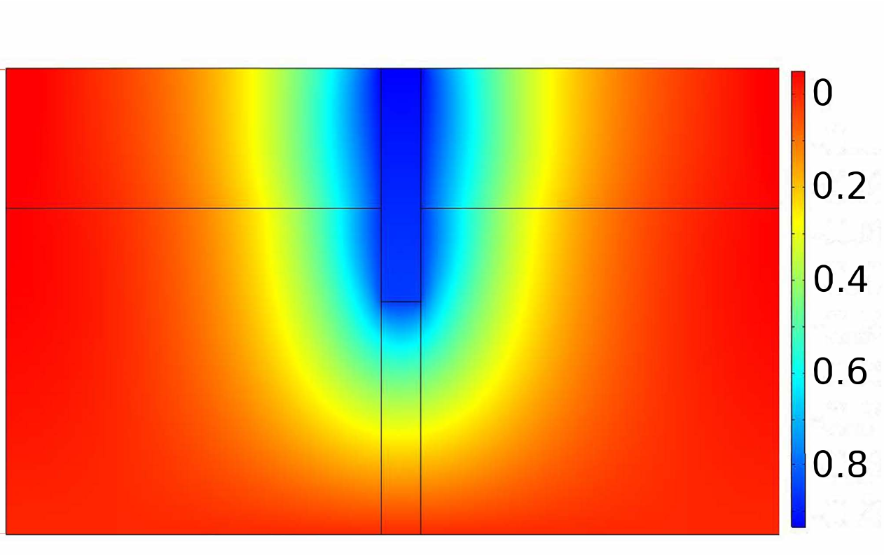
In Fig. 9, the training history of the normalized loss versus epochs and time is presented for the identification study. As can be seen, the relative error norm has reached below within epochs. This indicates a substantial reduction in convergence rate in comparison to the forward study, which is expected in inverse solutions. In Fig. 10, contours of the normalized vertical displacement field are presented for the backward solution and compared to the reference FEM solution using COMSOL. Evidently, the PINNs results are in excellent agreement with the reference solution. In table 1 the exact values of the Young’s modulus of the soil inverted in each case are reported. Notably, the deduced values in all cases lie within variation from the exact values.
In the last example, the application of PINNs to identify the material parameters of layered soils based on the inverse analysis of the axial strain profile measured/obtained along the pile is demonstrated. Consider a two-layered soil with the thickness ratios of and . The material properties of the domain are: Young’s Moduli of Elasticity, , , ; Poisson’s ratio, . Here, the equations governing the response of homogeneous soils (i.e., Eq.s (22)-(24)) need to be extended by inclusion of both soils layers (i.e., ). In particular, the contact constraints (i.e., Eq. (24)) need to be imposed across the interface of the pile with each soil layer as well as between the soil layers itself (see Eq. (16)). Such derivations are straightforward task, which is not presented here for the sake of brevity.
PINNs are employed to extract the Young’s moduli of both soils (i.e., and ). This inversion is again carried out by using a 1D data-set involving the strain (stress) profile across the center line of the pile. Six neural networks are elaborated for the PINNs solution in this example as
| (27) |
which consist of the same architecture as the previous case. The loss function is extended to incorporate both layers of the soil in conjunction with the additional contact constraints as
| (28) |
Sampling grid involves 3000 sampling points over , 2000 points in each of the soil layers and , and 2000 points due to the input data-set, which is summed at 9000 points in total. In Fig. 11, the training history of the normalized loss is presented. As can be seen, the convergence rate versus epochs has been relatively fast. Still, given the number of losses has expanded dramatically, the training is conducted significantly slower with respect to the case of inversion in homogeneous soils. Contours of the normalized vertical displacement field are depicted in Fig. 12 for both PINNs and reference solution by COMSOL. Evidently, excellent agreement is observed between the PINNs results and FE simulation. Finally, in Table 2 the inverted Young’s modulus for each soil layer is reported. The inverted values are in very good agreement with the precise amounts. This further demonstrates the excellent performance of PINNs in complex parametric studies pertaining to extremely limited input data.
| Analysis | |||
| Analysis 1. | 5.0 | 0.0213 | 0.02 |
| Analysis 2. | 5.0 | 0.105 | 0.10 |
| Analysis 3. | 5.0 | 0.525 | 0.5 |
| Analysis | |||||
| 5.0 | 0.095 | 0.1 | 0.023 | 0.02 |
5 Conclusions
A physics-informed deep learning framework is presented for the analysis of pile-soil interaction under vertical loading. In the framework, a domain-decomposition multi-network model is introduced to deal with the sharp discontinuities in the strain field at the interfaces of pile-soil regions and soil layers. The framework is trained by minimizing the loss function defined in terms of the equilibrium equations and the boundary conditions governing the pile-soil interaction problem. Several examples are provided to demonstrate the performance of the framework in the analysis of single piles embedded in homogeneous and layered soils under axisymmetric and plane strain conditions. Essential features of the framework are validated by comparing the PINN results with the results obtained from the finite element analysis. Good agreement is observed between the PINN and FEM results in all the cases considered. The application of the model for the inverse analysis and parameter identification of pile-soil interaction is also presented. In the examples provided, the localized data acquired along the pile length–possibly obtained via fiber optic strain sensing– is used for the inversion of soil parameters in both homogeneous and layered formations. As expected, a substantial reduction in the convergence rate is observed in the inverse analysis in comparison to the forward study. However, it is seen that the proposed PINN framework is able to identify the material parameters quite efficiently.
References
- Zienkiewicz et al. [1999] O. C. Zienkiewicz, A. Chan, M. Pastor, B. Schrefler, T. Shiomi, Computational geomechanics, volume 613, Citeseer, 1999.
- Ghasemi-Fare and Basu [2013] O. Ghasemi-Fare, P. Basu, A practical heat transfer model for geothermal piles, Energy and Buildings 66 (2013) 470–479.
- Rahmani and Pak [2012] A. Rahmani, A. Pak, Dynamic behavior of pile foundations under cyclic loading in liquefiable soils, Computers and Geotechnics 40 (2012) 114–126.
- Jafari et al. [2021] A. Jafari, M. Vahab, N. Khalili, Fully coupled xfem formulation for hydraulic fracturing simulation based on a generalized fluid leak-off model, Computer Methods in Applied Mechanics and Engineering 373 (2021) 113447.
- Calvello and Finno [2004] M. Calvello, R. J. Finno, Selecting parameters to optimize in model calibration by inverse analysis, Computers and Geotechnics 31 (2004) 410–424.
- Kabe [1985] A. M. Kabe, Stiffness matrix adjustment using mode data, AIAA journal 23 (1985) 1431–1436.
- Vardakos et al. [2012] S. Vardakos, M. Gutierrez, C. Xia, Parameter identification in numerical modeling of tunneling using the differential evolution genetic algorithm (dega), Tunnelling and underground space technology 28 (2012) 109–123.
- Walton and Sinha [2022] G. Walton, S. Sinha, Challenges associated with numerical back analysis in rock mechanics, Journal of Rock Mechanics and Geotechnical Engineering (2022).
- Lefik and Schrefler [2002] M. Lefik, B. A. Schrefler, Artificial neural network for parameter identifications for an elasto-plastic model of superconducting cable under cyclic loading, Computers & structures 80 (2002) 1699–1713.
- Gawin et al. [2001] D. Gawin, M. Lefik, B. Schrefler, Ann approach to sorption hysteresis within a coupled hygro-thermo-mechanical fe analysis, International Journal for Numerical Methods in Engineering 50 (2001) 299–323.
- Parish and Duraisamy [2016] E. J. Parish, K. Duraisamy, A paradigm for data-driven predictive modeling using field inversion and machine learning, Journal of computational physics 305 (2016) 758–774.
- Kardani et al. [2020] N. Kardani, A. Zhou, M. Nazem, S.-L. Shen, Estimation of bearing capacity of piles in cohesionless soil using optimised machine learning approaches, Geotechnical and Geological Engineering 38 (2020) 2271–2291.
- Momeni et al. [2015] E. Momeni, R. Nazir, D. J. Armaghani, H. Maizir, Application of artificial neural network for predicting shaft and tip resistances of concrete piles, Earth Sciences Research Journal 19 (2015) 85–93.
- Moayedi and Mosallanezhad [2017] H. Moayedi, M. Mosallanezhad, Uplift resistance of belled and multi-belled piles in loose sand, Measurement 109 (2017) 346–353.
- Das and Basudhar [2006] S. K. Das, P. K. Basudhar, Undrained lateral load capacity of piles in clay using artificial neural network, Computers and Geotechnics 33 (2006) 454–459.
- Armaghani et al. [2017] D. J. Armaghani, R. S. N. S. B. Raja, K. Faizi, A. S. A. Rashid, et al., Developing a hybrid pso–ann model for estimating the ultimate bearing capacity of rock-socketed piles, Neural Computing and Applications 28 (2017) 391–405.
- Cybenko [1989] G. Cybenko, Approximation by superpositions of a sigmoidal function, Mathematics of control, signals and systems 2 (1989) 303–314.
- Bishop [2006] C. M. Bishop, Pattern recognition and machine learning, springer, 2006.
- Goodfellow et al. [2016] I. Goodfellow, Y. Bengio, A. Courville, Y. Bengio, Deep learning, volume 1, MIT press Cambridge, 2016.
- Zhang et al. [2021] W. Zhang, H. Li, Y. Li, H. Liu, Y. Chen, X. Ding, Application of deep learning algorithms in geotechnical engineering: a short critical review, Artificial Intelligence Review (2021) 1–41.
- Azimi and Pekcan [2020] M. Azimi, G. Pekcan, Structural health monitoring using extremely compressed data through deep learning, Computer-Aided Civil and Infrastructure Engineering 35 (2020) 597–614.
- Bao et al. [2019] Y. Bao, Z. Tang, H. Li, Y. Zhang, Computer vision and deep learning–based data anomaly detection method for structural health monitoring, Structural Health Monitoring 18 (2019) 401–421.
- Li et al. [2019] X. Li, Z. Liu, S. Cui, C. Luo, C. Li, Z. Zhuang, Predicting the effective mechanical property of heterogeneous materials by image based modeling and deep learning, Computer Methods in Applied Mechanics and Engineering 347 (2019) 735–753.
- Zhang et al. [2018] D. Zhang, J. Lin, Q. Peng, D. Wang, T. Yang, S. Sorooshian, X. Liu, J. Zhuang, Modeling and simulating of reservoir operation using the artificial neural network, support vector regression, deep learning algorithm, Journal of Hydrology 565 (2018) 720–736.
- Azimi et al. [2018] S. M. Azimi, D. Britz, M. Engstler, M. Fritz, F. Mücklich, Advanced steel microstructural classification by deep learning methods, Scientific reports 8 (2018) 1–14.
- De Bézenac et al. [2019] E. De Bézenac, A. Pajot, P. Gallinari, Deep learning for physical processes: Incorporating prior scientific knowledge, Journal of Statistical Mechanics: Theory and Experiment 2019 (2019) 124009.
- Reichstein et al. [2019] M. Reichstein, G. Camps-Valls, B. Stevens, M. Jung, J. Denzler, N. Carvalhais, et al., Deep learning and process understanding for data-driven earth system science, Nature 566 (2019) 195–204.
- Karniadakis et al. [2021] G. E. Karniadakis, I. G. Kevrekidis, L. Lu, P. Perdikaris, S. Wang, L. Yang, Physics-informed machine learning, Nature Reviews Physics 3 (2021) 422–440.
- Sutton and Barto [2018] R. S. Sutton, A. G. Barto, Reinforcement learning: An introduction, MIT press, 2018.
- Han et al. [2018] J. Han, A. Jentzen, E. Weinan, Solving high-dimensional partial differential equations using deep learning, Proceedings of the National Academy of Sciences 115 (2018) 8505–8510.
- Haghighat et al. [2021] E. Haghighat, M. Raissi, A. Moure, H. Gomez, R. Juanes, A physics-informed deep learning framework for inversion and surrogate modeling in solid mechanics, Computer Methods in Applied Mechanics and Engineering 379 (2021) 113741.
- Owhadi [2015] H. Owhadi, Bayesian numerical homogenization, Multiscale Modeling & Simulation 13 (2015) 812–828.
- Bar-Sinai et al. [2019] Y. Bar-Sinai, S. Hoyer, J. Hickey, M. P. Brenner, Learning data-driven discretizations for partial differential equations, Proceedings of the National Academy of Sciences 116 (2019) 15344–15349.
- Rudy et al. [2017] S. H. Rudy, S. L. Brunton, J. L. Proctor, J. N. Kutz, Data-driven discovery of partial differential equations, Science Advances 3 (2017) e1602614.
- Raissi et al. [2019] M. Raissi, P. Perdikaris, G. E. Karniadakis, Physics-informed neural networks: A deep learning framework for solving forward and inverse problems involving nonlinear partial differential equations, Journal of Computational Physics 378 (2019) 686–707.
- Baydin et al. [2018] A. G. Baydin, B. A. Pearlmutter, A. A. Radul, J. M. Siskind, Automatic differentiation in machine learning: a survey, Journal of machine learning research 18 (2018).
- Abadi et al. [2016] M. Abadi, P. Barham, J. Chen, Z. Chen, A. Davis, J. Dean, M. Devin, S. Ghemawat, G. Irving, M. Isard, et al., Tensorflow: A system for large-scale machine learning, in: 12th USENIX symposium on operating systems design and implementation (OSDI 16), pp. 265–283.
- Chollet et al. [2015] F. Chollet, et al., keras, 2015.
- Haghighat and Juanes [2021] E. Haghighat, R. Juanes, Sciann: A keras/tensorflow wrapper for scientific computations and physics-informed deep learning using artificial neural networks, Computer Methods in Applied Mechanics and Engineering 373 (2021) 113552.
- Haghighat et al. [2021] E. Haghighat, A. C. Bekar, E. Madenci, R. Juanes, A nonlocal physics-informed deep learning framework using the peridynamic differential operator, Computer Methods in Applied Mechanics and Engineering 385 (2021) 114012.
- Vahab et al. [2022] M. Vahab, E. Haghighat, M. Khaleghi, N. Khalili, A physics-informed neural network approach to solution and identification of biharmonic equations of elasticity, Journal of Engineering Mechanics 148 (2022) 04021154.
- Khaleghi et al. [2022] M. Khaleghi, E. Haghighat, M. Vahab, B. Shahbodagh, N. Khalili, Fracture characterization from noisy displacement data using artificial neural networks, Engineering Fracture Mechanics 271 (2022) 108649.
- Mao et al. [2020] Z. Mao, A. D. Jagtap, G. E. Karniadakis, Physics-informed neural networks for high-speed flows, Computer Methods in Applied Mechanics and Engineering 360 (2020) 112789.
- Sahli Costabal et al. [2020] F. Sahli Costabal, Y. Yang, P. Perdikaris, D. E. Hurtado, E. Kuhl, Physics-informed neural networks for cardiac activation mapping, Frontiers in Physics 8 (2020) 42.
- Kharazmi et al. [2021] E. Kharazmi, Z. Zhang, G. E. Karniadakis, hp-vpinns: Variational physics-informed neural networks with domain decomposition, Computer Methods in Applied Mechanics and Engineering 374 (2021) 113547.
- Niaki et al. [2021] S. A. Niaki, E. Haghighat, T. Campbell, A. Poursartip, R. Vaziri, Physics-informed neural network for modelling the thermochemical curing process of composite-tool systems during manufacture, Computer Methods in Applied Mechanics and Engineering 384 (2021) 113959.
- Chen et al. [2020] Y. Chen, L. Lu, G. E. Karniadakis, L. Dal Negro, Physics-informed neural networks for inverse problems in nano-optics and metamaterials, Optics express 28 (2020) 11618–11633.
- Jagtap et al. [2020] A. D. Jagtap, E. Kharazmi, G. E. Karniadakis, Conservative physics-informed neural networks on discrete domains for conservation laws: Applications to forward and inverse problems, Computer Methods in Applied Mechanics and Engineering 365 (2020) 113028.
- Lou et al. [2021] Q. Lou, X. Meng, G. E. Karniadakis, Physics-informed neural networks for solving forward and inverse flow problems via the boltzmann-bgk formulation, Journal of Computational Physics (2021) 110676.
- Mohamad et al. [2011] H. Mohamad, K. Soga, A. Pellew, P. J. Bennett, Performance monitoring of a secant-piled wall using distributed fiber optic strain sensing, Journal of Geotechnical and Geoenvironmental Engineering 137 (2011) 1236–1243.
- Mohamad et al. [2012] H. Mohamad, K. Soga, P. J. Bennett, R. J. Mair, C. S. Lim, Monitoring twin tunnel interaction using distributed optical fiber strain measurements, Journal of geotechnical and geoenvironmental engineering 138 (2012) 957–967.
- Jagtap and Karniadakis [2021] A. D. Jagtap, G. E. Karniadakis, Extended physics-informed neural networks (xpinns): A generalized space-time domain decomposition based deep learning framework for nonlinear partial differential equations., in: AAAI Spring Symposium: MLPS, pp. 2002––2041.
- Wang et al. [2022] S. Wang, X. Yu, P. Perdikaris, When and why pinns fail to train: A neural tangent kernel perspective, Journal of Computational Physics 449 (2022) 110768.
- Multiphysics [1998] C. Multiphysics, Introduction to comsol multiphysics®, COMSOL Multiphysics, Burlington, MA, accessed Feb 9 (1998) 2018.