Quantum corrections to the Schwarzschild metric from vacuum polarization

The leading order contributions of the stress-energy tensor are expected to behave as $\langle\rho\rangle\sim O(\hbar^{1})$, $\langle p\rangle\sim O(\hbar^{1})$ [where $\langle p\rangle=\langle p_{r}\rangle=\langle p_{t}\rangle$]. We can thus look for perturbative solutions of the semiclassical TOV equations, solving the system order by order in powers of $\hbar$. In this subsection we will obtain the first order correction using analytical techniques, and in the next subsection we will analyze the validity of this approach by solving the system of equations numerically.

Solving the TOV equations at order $\hbar^{0}$ gives $m(r)=M+O(\hbar)$ and $\phi\sim-\frac{1}{2}\log({1-2M/r})+O(\hbar)$, where $M$ is an arbitrary constant of integration, which can be identified with the ADM mass. This is the Schwarzschild metric, as expected at order $\hbar^{0}$. To get something interesting we have to solve the equations at first order in $\hbar$. Let us define $m=M+m_{1}\hbar+O(\hbar^{2})$, $\phi\sim-\frac{1}{2}\log({1-2M/r})+\phi_{1}\hbar+O(\hbar^{2})$, $\langle\rho\rangle=\rho_{1}\hbar+O(\hbar^{2})$,$\langle p\rangle=p_{1}\hbar+O(\hbar^{2})$. Then the system of equations at first order in $\hbar$ is given by

	$\displaystyle\frac{dm_{1}}{dr}$	$\displaystyle=$	$\displaystyle 4\pi r^{2}\rho_{1}\,,$		(12)
	$\displaystyle\frac{d\phi_{1}}{dr}$	$\displaystyle=$	$\displaystyle-\frac{m_{1}}{r^{2}f^{2}}-\frac{4\pi rp_{1}}{f}\,,$		(13)
	$\displaystyle\frac{dp_{1}}{dr}$	$\displaystyle=$	$\displaystyle-\frac{M}{r^{2}f}(\rho_{1}+p_{1})\,,$		(14)
	$\displaystyle-\rho_{1}$	$\displaystyle+$	$\displaystyle 3p_{1}=\frac{M^{2}}{60\pi^{2}r^{6}}\,,$		(15)

where $f=1-\frac{2M}{r}$. This system can be solved analytically, obtaining the following expressions for the pressure and density ¹¹ 1 The negative sign and the dependence on $1/f^{2}$ obtained in these expressions are in agreement with the exact results obtained on the fixed (Schwarzschild) background near the horizon for the Boulware vacuum state [see (11)].

	$\displaystyle\langle p\rangle$	$\displaystyle=$	$\displaystyle-\frac{\hbar M^{3}}{480\pi^{2}r^{7}f^{2}}(\frac{1}{7}+f)+\mathcal{O}(\hbar^{2})\ ,$		(16)
	$\displaystyle\langle\rho\rangle$	$\displaystyle=$	$\displaystyle\hbar\left(-\frac{M^{3}}{160\pi^{2}r^{7}f^{2}}(\frac{1}{7}+f)-\frac{M^{2}}{60\pi^{2}r^{6}}\right)+\mathcal{O}(\hbar^{2})\ ,$		(17)

and the following ones for the metric components

	$\displaystyle m$	$\displaystyle=$	$\displaystyle M+\frac{\hbar}{40320\pi Mf}\left(9-36f\log(f)+10f-174f^{2}+246f^{3}-91f^{4}\right)+O(\hbar^{2})\,,$		(18)
	$\displaystyle\phi$	$\displaystyle=$	$\displaystyle-\frac{1}{2}\log f+\frac{\hbar}{80640\pi M^{2}f^{2}}\left(3+36(-1+3f)f\log(f)-35f+152f^{2}-132f^{3}+5f^{4}+7f^{5}\right)+O(\hbar^{2})\,.$		(19)

To fix the constants of integration we have assumed the natural boundary conditions $\langle p\rangle(r\to\infty)=0$, $\langle\rho\rangle(r\to\infty)=0$ and the metric tending to the Schwarzschild one as $r\to\infty$. For pedagogical purposes, we display the asymptotic form of the metric around $r=2M$

$$ds^{2}=-\left(f(r)-\hbar\left(\frac{1}{13440\pi M^{2}f(r)}+\mathcal{O}(\log f)\right)+\mathcal{O}(\hbar^{2})\right)dt^{2}+\frac{dr^{2}}{f(r)-\hbar\left(\frac{1}{4480\pi M^{2}f(r)}+\mathcal{O}(\log f)\right)+\mathcal{O}(\hbar^{2})}+r^{2}d\Omega^{2}\,.$$

(20)

In the Appendix A we prove that the curvature at this singular point is finite, so this is just a coordinate singularity. In fact, this is just the classical Schwarzschild coordinate singularity at $r=2M$ shifted to the value $r_{0}$ defined by $g_{rr}^{-1}(r_{0})=0$. Using the expression (18) and imposing $2m(r_{0})=r_{0}$, we easily obtain

$$r_{0}=2M+\frac{\sqrt{\hbar}}{4\sqrt{70\pi}}+\mathcal{O}(\hbar)\ .$$

(21)

In geometrized units $\sqrt{\hbar}=l_{p}$ is the Planck length. This singular, limiting point defines the end of validity of our coordinate system, which would traditionally indicate the location of a “horizon” at $r=r_{0}$. However, note that, unlike the Schwarzschild case, in this point the component $g_{tt}$ of the metric (the so called redshift function) does not vanish, but takes the value

$$g_{tt}(r_{0})=-\frac{\sqrt{\hbar}}{12\sqrt{70\pi}M}+\mathcal{O}(\hbar)\,.$$

(22)

This implies that the static spacetime that we have obtained does not contain a horizon, i.e. it is not defining a black hole Vishveshwara. We check this in the Appendix A.

Note that, even though (16)-(17) are generally very small (because of the prefactor $\hbar$), they become relevant around $r\sim r_{0}$, since in this limit the factor $f(r)$ in the denominator can compensate $\hbar$. In other words, quantum effects are quite important near the location of what was classically the horizon. The Krechtmann scalar is also found to be significantly corrected at the singular point (see Appendix A). These observations lead us to the following subsection.

As we can see the results obtained above at first order in $\hbar$ also depend on $f(r)$, which takes values of order $\sqrt{\hbar}$ near the singular point $r=r_{0}$. This dependence compensates the small value of $\hbar$ in some expressions above. Because of this, a natural question is whether the perturbative method is a good approximation near to the singular point. To answer this we can solve the TOV equations at second order in $\hbar$ and analyze whether near the singular point the solution is consistent with the perturbative hypothesis (i.e. that the order $\hbar^{1}$ is larger than the order $\hbar^{2}$, etc.). The analysis is tedious and we avoid showing the details. What we obtain is that the $\hbar^{2}$ contribution to the pressure and the density is proportional to $\hbar^{2}/{f(r)^{4}}$. Near to the singular point $f(r)^{4}$ is of order $\hbar^{2}$, so this term competes with the first order contribution (16), which is proportional to $\hbar/f(r)^{2}$. Therefore we find that, near the singular point, the higher order contributions in $\hbar$ are not necessarily smaller than the first one and perturbation theory actually breaks down. Therefore, we cannot rely on the perturbative series in the vicinity of $r_{0}$ and we are forced to solve the differential TOV equations exactly, which can only be done numerically. Still, we shall find that the perturbative approach presented in the previous subsection is a good approximation to the problem, and it qualitatively predicts well the behavior of the nonperturbative solution.²² 2 In this paper we work in the semiclassical regime in which fluctuations of the stress-energy tensor are negligible compared to its mean value. Going beyond this framework would require working with techniques in stochastic gravity hu-verdaguer, which is out of the scope of the present paper. By nonperturbative we mean the exact solution of the TOV equations within the semiclassical framework.

We now turn to solve numerically the TOV equations (4)-(6) using the equation of state (10) and $\langle p_{r}\rangle=\langle p_{t}\rangle$. We place the boundary conditions at $r=1000M$, and demand that at this location the solution is approximately the Schwarzschild metric³³ 3 To get more precision we can choose the corrected solution at first order in $\hbar$ obtained above, but the results near the singular point are numerically indistinguishable.. An important issue that one faces when solving the equations numerically is that the value of $\hbar$ is much smaller than $M$. To be able to distinguish the implications of a nonzero but tiny value of $\hbar$ from the numerical error, one needs a huge computer accuracy. To avoid this issue, a useful strategy is to use first some artificial high values of $\hbar$ (between $10^{-5}M^{2}$ and $10^{-15}M^{2}$), study the dependence of the results on $\hbar$, and then extrapolate the relevant quantities to the actual value of $\hbar$. By solving numerically the equations for different values of $\hbar$ and calculating for each case the value of $r_{0}$ we obtain results that approximately fit the expression $r_{0}\approx 2M+0.01947\sqrt{\hbar}$. This shift differs from the one estimated by the perturbative method ($r_{0}\approx 2M+0.01686\sqrt{\hbar}$) but the functional dependence on $\hbar$ remains the same.

In Fig. 1 we plot the components of the metric obtained numerically, normalized by the factor $f(r)=1-2M/r$, as well as the renormalized energy density and pressure. They are plotted as a function of $\epsilon=\frac{r-2M}{\sqrt{\hbar}}$. With this new radial variable the singular point $r_{0}$ does not depend on the specific value of $\hbar$. These plots are taken for $\hbar/M^{2}=10^{-5}$, but we have analyzed them for other values and have seen that they do not significantly depend on the chosen value of $\hbar$ near the singular point. From these plots one can see that, as in the perturbative solution, the component $g_{rr}^{-1}$ tends to 0 at the singular point $r=r_{0}$, while $g_{tt}$ tends to a nonzero value. The energy density and pressure differ from 0 as they approach the singular point, as expected. More precisely $g_{tt}\sim O(\sqrt{\hbar}/M)$, $g^{-1}_{rr}\sim(r-r_{0})/M$, $\rho\sim O(\hbar^{0})$, and $p\sim O(\hbar^{0})$ as $r\to r_{0}$. This is the same dependence on $\sqrt{\hbar}/M$ as that obtained by the perturbative approach, although the numerical coefficients are different. This allows us to consider the perturbative solution as a qualitatively good approximation.

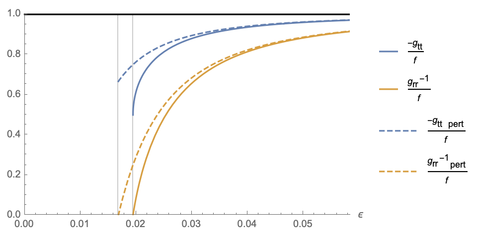
We can summarize the above numerical result in terms of the following generic expression for the metric

$$ds^{2}=g_{tt}dt^{2}+g_{rr}dr^{2}+r^{2}d\Omega^{2}\ ,$$

(23)

where $g^{-1}_{rr}\to 0$, as $r\to r_{0}>2M$ and $g_{tt}(r_{0})\neq 0$. Furthermore, $g^{-1}_{rr}\ \sim(r-r_{0})/M$ and $g_{tt}(r)\sim\mathcal{O}(\sqrt{\hbar}/{M})$ in a neighborhood of $r_{0}$.

Instead of working with the metric ansatz (2) and then transforming to (24) by a change of variables, we can alternatively solve the problem from scratch using the latter metric directly and explore if there exist wormhole solutions. The equivalent system of TOV equations now reads (we find convenient to introduce the defining relation $g(l)\equiv\frac{dr}{dl}$)

	$\displaystyle\frac{dr}{dl}$	$\displaystyle=$	$\displaystyle g\,,$		(25)
	$\displaystyle\frac{dg}{dl}$	$\displaystyle=$	$\displaystyle\frac{1-8\pi r^{2}\left<\rho\right>+g^{2}}{2r}\,,$		(26)
	$\displaystyle\frac{d\phi}{dl}$	$\displaystyle=$	$\displaystyle\frac{-1-8\pi r^{2}\left<p_{r}\right>+g^{2}}{2rg}\,,$		(27)
	$\displaystyle\frac{d\left<p_{r}\right>}{dl}$	$\displaystyle=$	$\displaystyle\frac{(-1-8\pi r^{2}\left<p_{r}\right>+g^{2})(\left<p_{r}\right>+\left<\rho\right>)}{2rg}+\frac{2g(\left<p_{t}\right>-\left<p_{r}\right>)}{r}\,.$		(28)

There are six unknowns for four equations. Again, we can impose two equations of state to get a solvable model. As before, we shall take $\left<p_{t}\right>=\left<p_{r}\right>$ (notice that the contribution of $\langle p_{t}\rangle-\langle p_{r}\rangle$ is negligible near the throat, where as we will see $g(0)=0$) and $\left<T^{a}_{a}\right>$ given by the trace anomaly:

$$-\langle\rho\rangle+3\langle p\rangle=\frac{\hbar}{180}\left[\frac{1-g^{2}}{2\pi r^{2}}\left(3\frac{1-g^{2}}{2\pi r^{2}}-8\langle\rho\rangle\right)+8\langle\rho\rangle(\langle p\rangle+\langle\rho\rangle)\right]\,.$$

(29)

To get wormhole solutions we must impose several conditions. Without loss of generality, we can locate the throat at $l=0$. One of the sectors of the throat (that would represent the universe we live in) must be asymptotically flat, and inertial observers at infinity must measure time with $t$. We choose that sector corresponding to $l>0$. Then the previous condition requires $\phi(\infty)=0$, $\left<p_{r}\right>(\infty)=\left<\rho\right>(\infty)=0$. On the other hand, the coordinate $l$ should agree with the radial function $r(l)$ at infinity, i.e. $r(l)\to l$ as $l\to\infty$. Furthermore, for sufficiently large distances away from the throat, $g$ must be given by the Morris-Thorne coordinate transformation (the solution should mimic a black hole at large distances), i.e. $g(l)\sim\sqrt{1-2m(l)/l}$ and therefore $g(\infty)=1$.

This set of boundary conditions, together with the two equations of state specified above, can be used to obtain a unique solution to the above system of differential equations, integrating all the way down from $l=+\infty$ until negative values of $l$. Notice that in general there will be no mirror-reflection symmetry at the throat. The results are shown in the next subsection. For the solution to represent a wormhole, note that i) the throat must have a finite, nonvanishing radius, so $r(0)=r_{0}>0$, and ii) the throat area must correspond to a minimum, therefore $g(0)=0$.

Before discussing the results, we remark an important issue. It may seem that the above system of equations is not well defined at the throat $l=0$ because of $g(0)=0$ in the denominator of some equations. But notice that, according to Einstein’s equation,

$\displaystyle\left<p_{r}(r)\right>=-\frac{1}{8\pi}\left[\frac{2m}{r^{3}}-2\left(1-\frac{2m}{r}\right)\frac{\partial_{r}\phi}{r}\right]\,,$

(30)

so at the throat (where $2m(r)=r$) we also have $p_{r}(0)=-1/(8\pi r_{0}^{2})$, provided that $\partial_{r}\phi(0)$ is well-defined at the throat or that it does not blow up as quickly as $(1-2m/r)^{-1}$ (this is verified in this case, using the numerical solution obtained in the previous section one can see that $\partial_{r}\phi\sim(1-2m(r)/r)^{-1/2}$ when $r\to r_{0}$). Therefore, the numerator of (27) and (28) also vanishes whenever the denominator does, and we have a $0/0$ ambiguity. To ensure that we can extend the metric across the throat one needs to check first that the limit $l\to 0$ tends to a finite value under the boundary conditions specified above. Numerically we find that near the throat $1+8\pi r^{2}p\sim O(l)$ and $g\sim O(l)$, so we can conclude that the limit of the quotient will be finite.

In Fig. 2 we show the result of solving numerically the system of equations (25),(26),(27),(28) and (29) under the conditions specified in the previous subsection. As in Sec III. B, to capture the implications of a nonvanishing but tiny value of $\hbar$ on the equations, we do the calculation for several high values of $\hbar$ (so that their effect is numerically distinguishable), then we perform a fit of the results to be able to extrapolate the value of interest with the actual value of Planck’s constant. In our calculation the throat is located at $l=0$, note how at this point there is a bounce in the function $r(l)$ (its derivative $g(l)$ changes sign).

Furthermore, we find that in the interior region, $l<0$, a new singular point appears at $l_{s}\sim-0.278\,\hbar^{1/4}\sqrt{M}$. It is a singular point because the redshift function vanishes there, $g_{tt}(l_{s})=0$. As we approach to $l_{s}$ we find that the renormalized density, the pressure and the scalar of curvature $R=8\pi(-\rho+3p)$ all tend to diverge. This signals the existence of a curvature singularity. To confirm the existence of this singularity from an analytical viewpoint we can examine the expression of the scalar curvature in terms of the metric components:

$$R(l)=\frac{g_{tt}^{\prime}(l)^{2}}{2g_{tt}(l)^{2}}-\frac{g_{tt}^{\prime\prime}(l)r(l)+2g_{tt}^{\prime}(l)r^{\prime}(l)}{g_{tt}(l)r(l)}-\frac{2\left(2r(l)r^{\prime\prime}(l)+r^{\prime}(l)^{2}-1\right)}{r(l)^{2}}\,.$$

(31)

Since at the singular point $g_{tt}(l_{s})=0$ (see Fig. 2) some terms of this expression diverge at this point. Although $g_{tt}^{\prime}(l)$ also vanishes at $l=l_{s}$, numerical computations show that it decreases slower than $g_{tt}(l)$. To see the causal character of this curvature singularity, let us consider the induced metric on a $l=$ constant three-dimensional hypersurface: $d\bar{s}^{2}=g_{tt}(l)dt^{2}+r(l)^{2}d\Omega^{2}$. At the singularity $l=l_{s}$ we have $g_{tt}(l_{s})=0$, so the metric becomes degenerate: $d\bar{s}^{2}=0+r(l_{s})^{2}d\Omega^{2}$. Therefore, the surface $l=l_{s}$ becomes a null hypersurface Galloway, and this curvature singularity is null. Fig. 3 provides a Penrose diagram that shows all these features.

An important question is how long it would take for an observer crossing the throat to reach this curvature singularity. To study this let us consider a radial and timelike geodesic starting at $l=0$ (throat) and ending at the singular point $l=l_{s}$. The relevant geodesic equation for a static and spherically symmetric metric $ds^{2}=g_{tt}(l)dt^{2}+g_{ll}(l)dl^{2}+r(l)^{2}d\Omega^{2}$ is given by

$$\frac{dl}{d\tau}=\pm\sqrt{-g_{ll}^{-1}(E^{2}g_{tt}^{-1}+\frac{L^{2}}{r^{2}}+\mu)}$$

(32)

where $\tau$ is the proper time, $\mu=+1,0,-1$ for timelike, null and spacelike geodesics respectively, and $E$ and $L$ are constants of motion given by $E=-g_{tt}\frac{dt}{d\tau}$ and $L=r^{2}\frac{d\phi}{d\tau}$. In our case $g_{ll}=1$, $\mu=1$, $L=0$, and $dl/d\tau<0$ (the geodesic is approaching the singularity), so

$$\frac{dl}{d\tau}=-\sqrt{E^{2}g_{tt}(l)^{-1}-1}\,.$$

(33)

The proper time needed to reach the curvature singularity from the throat is then given by

$$\Delta\tau=-\int_{0}^{l_{s}}\frac{dl}{\sqrt{E^{2}g_{tt}(l)^{-1}-1}}\,.$$

(34)

(the condition that the geodesic propagates into the future, $\partial_{\tau}t>0$, implies $E^{2}g_{tt}(l)^{-1}>1$ and guarantees that the integral is real). The order of magnitude of this quantity can be estimated as follows. From (22) we know that $g_{tt}(0)\sim\sqrt{\hbar}/M$. Assuming $E\sim 1$, we have $E^{2}g_{tt}^{-1}(l)>>1$ in the region of the integration. Since $|l_{s}|\sim\hbar^{1/4}\sqrt{M}<<1$ we can also Taylor expand the integral to finally get

$$\Delta\tau\sim-\int_{0}^{l_{s}}\sqrt{g_{tt}(l)}dl\sim\sqrt{g_{tt}(0)}|l_{s}|+O(l_{s}^{2})\sim\sqrt{\hbar}$$

(35)

So an observer crossing the throat will almost immediately see the presence of the curvature singularity.

Finally, we want to stress that the occurrence of the curvature singularity has been obtained for a purely vacuum semiclassical solution. The presence of matter producing very compact stellar objects (ECOs) makes only the outer part of the solution physically relevant. Moreover, these results also suggest a maximum in the compactness of ECOs. This maximum would be given by the minimum of the radial function $r(l)$, i.e. the throat ($r=r_{0}$). Therefore this maximum of compactness (measured as $2M/r(l)$) is of order

$$\frac{2M}{r_{0}}\sim 1-0.01686\frac{\sqrt{\hbar}}{2M}\ .$$

(36)

We regard (36) as one of the main results of this work. Probing the exterior of the semiclassical metric via scalar and vector perturbations will be the topic of the next section.

Remark: Another way to extend the metric beyond the coordinate singularity $r=r_{0}$ consists in defining a coordinate $\bar{r}$ by $\frac{d\bar{r}}{dr}=e^{-\phi(r)}(1-\frac{2m(r)}{r})^{-1/2}$. In this case the metric has the form

$$ds^{2}=-G(\bar{r})dt^{2}+\frac{dr^{2}}{G(\bar{r})}+R(\bar{r})^{2}d\Omega^{2}\,.$$

(37)

Using this metric as an ansatz for solving the semiclassical TOV equations we found that the functions $G$ and $R$ can be analitically extended beyond the coordinate singularity $\bar{r}=\bar{r}_{0}$. In particular $R(\bar{r})$ reaches a minimum at $\bar{r}_{0}$ and starts increasing for lower values, as expected for a wormhole metric. On the other hand $G(\bar{r})$ continues to decrease until it reaches the value $\bar{r}=\bar{r}_{s}$, where $G(\bar{r}_{s})=0$. At this point we again find a curvature singularity, which is equivalent to the one found in the other extension explained above. Therefore, with this alternative extension, we obtain the same conclusions. However the approach described above allows a higher accuracy in the numerical calculations.

Let us study the behavior of a massless scalar field coupled to a general static and spherically symmetric background, $ds^{2}=g_{tt}dt^{2}+g_{rr}dr^{2}+r^{2}d\Omega^{2}$. The field satisfies the Klein-Gordon equation

$$(\Box+\xi R)\phi=0\,.$$

(38)

Since the metric is static and spherically symmetric, we can look for solutions of the following form

$$\phi_{\omega lm}=\frac{1}{r}e^{-i\omega t}Y_{lm}(\theta,\psi)\Psi_{\omega l}(r)\,.$$

(39)

For a curved spacetime the D’Alembert operator is given by $\Box\phi=\frac{1}{\sqrt{-g}}\partial_{\mu}(\sqrt{-g}g^{\mu\nu}\partial_{\nu}\phi)$. The Klein-Gordon equation decouples and, after some calculations one obtains the following equation for the radial function

$$F^{2}\Psi_{\omega l}^{\prime\prime}+FF^{\prime}\Psi_{\omega l}^{\prime}+(\omega^{2}-V_{l})\Psi_{\omega l}=0\,,$$

(40)

where

	$\displaystyle F(r)=\sqrt{-\frac{g_{tt}}{g_{rr}}}\,,$		(41)
	$\displaystyle V(r)=-g_{tt}(r)\left(\frac{l(l+1)}{r^{2}}-\xi R(r)\right)+\frac{F(r)F^{\prime}(r)}{r}\,.$		(42)

If we define a generalized tortoise coordinate as $\partial_{r^{*}}=F(r)\partial_{r}$, then Eq.(40) can be rewritten in the usual Regge-Wheeler form $\partial_{r_{*}}^{2}{\Psi}_{\ell m}+(\omega^{2}-V){\Psi}_{\ell m}=0$. In particular, for a Schwarzschild background we recover the usual expression.

Now let us study this potential for our particular case, given by $g_{tt}=-e^{-2\phi(r)}$ and $g_{rr}=1-\frac{2m(r)}{r}$, where $\phi(r)$ and $m(r)$ have been obtained in Sec. III. Using the semiclassical TOV equations we can rewrite the potential as

$$V(r)=e^{-2\phi(r)}\left(\frac{l(l+1)}{r^{2}}+\frac{2m(r)}{r^{3}}+4\pi\left((1-6\xi)\langle p(r)\rangle+(-1+2\xi)\langle\rho(r)\rangle\right)\right)\,.$$

(43)

It is easy to see that in the Schwarzschild limit $\hbar\to 0$ this expression reduces to the usual effective potential for scalar fields. We can now use the perturbative solution of the corrected Schwarzschild metric to obtain the correction of the Regge-Wheeler potential at first order in $\hbar$. The resulting expression, at first order in $\hbar$, yields

	$\displaystyle V(r)$	$\displaystyle=$	$\displaystyle V_{0}(r)+\frac{\hbar}{20160\pi M^{2}r^{6}f}\biggl[-2688M^{4}\xi f^{2}+Mr^{3}\biggl(-3\lambda+(53+32\lambda)f-40(1+3\lambda)f^{2}+12(-36+\lambda)f^{3}$		(44)
		$\displaystyle+$	$\displaystyle(664+7\lambda)f^{4}-245f^{5}\biggr)+18r^{4}\left((1+\lambda)-(5+3\lambda)f+4f\right)f\log(f)\biggr]+O\left(\hbar^{2}\right)\,,$

where $f=1-\frac{2M}{r}$, $\lambda=l(l+1)$ and $V_{0}(r)=f(\frac{\lambda}{r^{2}}+\frac{2M}{r^{3}})$, which is the effective potential for scalar fields on a Schwarzschild background. Note that this expression does not depend on $\xi$. This is because the scalar curvature is given by $R=8\pi(-\rho+3p)$, and expanding around $r=2M$ we have $\rho\approx 3p$ at leading order (see (17) and (16)), so the term $\xi R$ is subleading. On the other hand, near the throat $f(r_{0})\sim O(\sqrt{\hbar}/M)$ so the quantum correction of the effective potential is of order $O(\sqrt{\hbar}/M^{3})$ near the throat, while it is of order $O(\hbar/M^{4})$ in general.

Using this expression for the corrected effective potential, we can now obtain the quantum corrections at first order in $\hbar$ to the light ring frequencies. The computation of these frequencies requires numerical methods. However, one can obtain a reasonable estimation by using the WKB approximation iyer-will.

Let us briefly review the calculation for a Schwarzschild metric. In this framework the light ring frequencies at $0-$th adiabatic order are given by

$$\omega_{n}^{2}=V(r^{*}_{m})-i\sqrt{-2V^{\prime\prime}(r^{*}_{m})}(n+\frac{1}{2})\,,$$

(45)

where $r^{*}_{m}$ is the value of the tortoise coordinate at which the potential is maximum, and the primes mean derivatives with respect to $r^{*}$. In the case of a Schwarzschild background the maximum of the potential is located at

$$r_{m}=\frac{3(\lambda-1)+\sqrt{(9\lambda+14)\lambda+9}}{2\lambda}M\,,$$

(46)

which for large $l$ tends to $r_{m}\sim 3M$. [The case $\lambda=0$ ($l=0$) has to be studied separately, we analyze it at the end of this section]. Using this expression, we can obtain the frequency of the light-ring modes for a scalar perturbation in a classical black hole

$$\small{\omega_{Sch}^{2}=\frac{1}{M^{2}}\left(1-\frac{2}{\tilde{r}_{m}}\right)\left(\frac{\lambda}{\tilde{r}_{m}^{2}}+\frac{2}{\tilde{r}_{m}^{3}}\right)-i\left(n+\frac{1}{2}\right)\frac{2}{M^{2}\tilde{r}_{m}^{4}}\sqrt{\left(1-\frac{2}{\tilde{r}_{m}}\right)\left(-96\tilde{r}_{m}-10(3\lambda-7)\tilde{r}_{m}^{2}+4(5\lambda-3)\tilde{r}_{m}^{3}-3\lambda\tilde{r}_{m}^{4}\right)}}\,,$$

(47)

where $\tilde{r}_{m}=r_{m}/M$.

References

- (1) B. P. Abbott et al. (LIGO Scientific Collaboration and Virgo Collaboration) Phys. Rev. Lett. 116, 061102 (2016).
- (2) The Event Horizon Telescope Collaboration et al., Astrophys.J.Lett. 875, L1 (2019).
- (3) V. Cardoso and P. Pani, Living Rev. Relativity 22, 4 (2019).
- (4) S. L. Shapiro, S. L. and S. A. Teukolsky, Black Holes, White Dwarfs, and Neutron Stars: The Physics of Compact Objects (Wiley, New York, 1983).
- (5) F. E. Schunck, and E. W. Mielke, Classical Quantum Gravity 20, R301 (2003).
- (6) G. Raposo, P. Pani, M. Bezares, C. Palenzuela, and V. Cardoso, Phys. Rev. D 99, 104072 (2019).
- (7) P. O. Mazur and E. Mottola, Proc. Natl. Acad. Sci. U.S.A. 101, 9545 (2004); Classical Quantum Gravity 32, 215024 (2015).
- (8) B. Holdom and J. Ren, Phys. Rev. D 95, 084034 (2017).
- (9) S. D. Mathur, Fortschr. Phys. 53, 793 (2005).
- (10) R. Brustein and A. J. M. Medved, Fortschr. Phys. 65, 1600114 (2017).
- (11) N. D. Birrel and P.C.W. Davies Quantum Fields in Curved Space (Cambridge University Press, Cambridge, England, 1984).
- (12) L. Parker and D. Toms Quantum Field Theory in Curved Spacetime ( Cambridge University Press, Cambridge, England, 2009).
- (13) B-L. Hu and E. Verdaguer, Semiclassical and Stochastic Gravity: Quantum Field Effects on Curved Spacetime ( Cambridge University Press, Cambridge, England, 2020).
- (14) P. R. Anderson, W. A. Hiscock and D. A. Samuel, Phys.Rev.D 51, 4337 (1995).
- (15) A. Levi and A. Ori, Phys. Rev. D 91, 104028 (2015).
- (16) A. Levi, E. Eilon, A. Ori and M. van de Meent, Phys. Rev. Lett. 118, 141102 (2017).
- (17) A. Fabbri and J. Navarro-Salas, Modeling Black Hole Evaporation (ICP-World Scientific, London, England, 2005).
- (18) A. Fabbri, S. Farese, J. Navarro-Salas, G. J. Olmo and H. Sanchis-Alepuz, Phys. Rev. D 73, 104023 (2006); J. Phys.: Conf. Ser. 33, 457 (2006).
- (19) P.M. Ho and Y. Matsuo, Classical Quantum Gravity 35, 065012 (2018).
- (20) J. Arrechea, C. Barceló, R. Carballo-Rubio and L.J.Garay, Phys. Rev. D 101, 064059 (2020).
- (21) R. Carballo-Rubio, Phys. Rev. Lett. 120, 061102 (2018).
- (22) P.M. Ho and Y. Matsuo, J. High Energy Phys. 03, 096 (2018).
- (23) J. Arrechea, C. Barceló, R. Carballo-Rubio and L.J.Garay, Phys. Rev.D 104, 084071 (2021); Sci. Rep. 12, 15958 (2022).
- (24) P.M. Ho, H. Kawai, Y. Matsuo. and Y. Yokokura, J. High Energy Phys. 11, 056 (2018).
- (25) J. L. Jaramillo, R. P. Macedo and L. A. Sheikh, Phys. Rev. X 11, 031003 (2021); Phys. Rev. Lett. 128, 211102 (2022).
- (26) V. Boyanov, K. Destounis, R. P. Macedo, V. Cardoso and J. L. Jaramillo, Phys. Rev. D 107, 064012 (2023).
- (27) I. Agullo, V. Cardoso, A. del Rio, M. Maggiore and J. Pullin, Phys. Rev. Lett. 126, 041302 (2021); Int. J. Mod. Phys. D 30, 2142013 (2021).
- (28) S. Chakraborty, E. Maggio, A. Mazumdar and P. Pani, Phys. Rev. D 106, 024041 (2022); R. Dey, S. Chakraborty, N. Afshordi, Phys. Rev. D 101, 104014 (2020).
- (29) B. Schutz, A First Course in General Relativity (Cambridge University Press, Cambridge, England, 2009).
- (30) P. Candelas Phys.Rev.D 21, 2185 (1980).
- (31) S.M. Christensen and S.A. Fulling, Phys. Rev. D 15, 2088 (1977).
- (32) R. M. Wald, Phys. Rev.D 17, 1477 (1978).
- (33) P. R. Anderson, R. Balbinot and A. Fabbri, Phys. Rev. Lett. 94, 061301 (2005).
- (34) C. V. Vishveshwara, J. Math. Phys. (N.Y.) 9, 1319 (1968).
- (35) Matt Visser, Lorentzian Wormholes: From Einstein to Hawking (Washington University, St. Louis, 1995).
- (36) F. S. N. Lobo, Wormholes, Warp Drives and Energy Conditions (Springer, Berlin, 2017), Vol. 189.
- (37) G. Galloway, Ann. Henri Poincaré 1, 543 (2000).
- (38) V. Cardoso, E. Franzin and P. Pani, Phys. Rev. Lett. 116, 171101 (2016); 117, 089902(E) (2016).
- (39) G. Khanna and R. H. Price Phys. Rev. D 95, 081501 (2017).
- (40) S. Iyer and C. M. Will, Phys. Rev. D 35, 3621 (1987); S. Iyer, Phys. Rev. D 35, 3632 (1987).
- (41) E. Berti, V. Cardoso and A. O. Starinets, Classical Quantum Gravity 26, 163001 (2009).
- (42) I. Agullo, A. del Rio and J. Navarro-Salas, Phys. Rev. Lett. 118, 111301 (2017); Phys. Rev. D 98, 125001 (2018).
- (43) J. Arrechea, C. Barcelo, R. Carballo-Rubio and L. J. Garay, Phys. Rev. D 107, 085005 (2023).