Transient Radio Lines from Axion Miniclusters and Axion Stars Preprint: FERMILAB-PUB-22-908-T
Abstract
Gravitationally bound clumps of dark matter axions in the form of ‘miniclusters’ or even denser ‘axion stars’ can generate strong radio signals through axion-photon conversion when encountering highly magnetised neutron star magnetospheres. We systematically study encounters of axion clumps with neutron stars and characterise the axion infall, conversion and the subsequent propagation of the photons. We show that the high density and low escape velocity of the axion clumps lead to strong, narrow, and temporally characteristic transient radio lines with an expected duration varying from seconds to months. Our work comprises the first end-to-end modeling pipeline capable of characterizing the radio signal generated during these transient encounters, quantifying the typical brightness, anisotropy, spectral width, and temporal evolution of the radio flux. The methods developed here may prove essential in developing dedicated radio searches for transient radio lines arising from miniclusters and axion stars.
I Introduction
Despite comprising over of the energy density in the Universe, the fundamental nature of dark matter remains unknown Aghanim et al. 2020a. Among the most well-motivated candidates for dark matter is the axion – a light pseudoscalar arising from a broken global symmetry that was originally introduced to solve the strong CP problem (i.e. the question of why quantum chromodynamics seems to conserve charge-parity symmetry) Peccei and Quinn 1977a; Peccei and Quinn 1977b; Weinberg 1978; Wilczek 1978.
Axion dark matter can be abundantly produced via various non-thermal processes in the early Universe, including the misalignment mechanism and the decays of topological defects (i.e. cosmic strings and domain walls) Preskill et al. 1983; Abbott and Sikivie 1983; Dine and Fischler 1983; Davis 1986; Lyth 1992. In the event that the global Peccei-Quinn symmetry is broken after the end of inflation, one expects these production mechanisms to generate modest fluctuations in the axion density field; the produced over-densities can subsequently undergo gravitational collapse near matter-radiation equality to source small virialized structures known as ‘axion miniclusters’ Hogan and Rees 1988; Kolb and Tkachev 1993; Kolb and Tkachev 1994a; Kolb and Tkachev 1994b; Kolb and Tkachev 1996; Zurek et al. 2007; Hardy 2017; O’Hare and Green 2017; Dokuchaev et al. 2017; Fairbairn et al. 2018; Vaquero et al. 2019; Eggemeier et al. 2020; Buschmann et al. 2020; Xiao et al. 2021; Ellis et al. 2022. As the miniclusters subsequently relax, the central regions of these objects can condense and form stable high-density cores known as ‘axion stars’ Kaup 1968; Ruffini and Bonazzola 1969; Tkachev 1986; Kolb and Tkachev 1993; Seidel and Suen 1994; Barranco and Bernal 2011; Levkov et al. 2018; Eggemeier and Niemeyer 2019; Chen et al. 2021; Braaten et al. 2016; Schiappacasse and Hertzberg 2018; Visinelli et al. 2018.
Recent years have shown significant progress in simulating the dynamics of the axion field in the early Universe, leading to estimates of the fraction of axion dark matter that collapses into miniclusters Vaquero et al. 2019; Buschmann et al. 2020; Xiao et al. 2021 in the post-inflationary Peccei-Quinn symmetry breaking scenario. A majority of these miniclusters are expected to survive until today – the notable exception being those which pass through dense stellar environments (such as found in the center of galaxies), where stellar encounters can efficiently strip and disrupt even the densest cores Kavanagh et al. 2021; Dandoy et al. 2022; Shen et al. 2022. Notice that the value of plays an important role in determining how and where to search for axion dark matter; in the limit , the local dark matter density is expected to tend toward zero (this is a consequence of the fact that Earth is statistically unlikely to be embedded in such an object), meaning the sensitivity of laboratory-based searches for axion dark matter may be severely reduced, or even eliminated entirely (although a recent study has suggested that the local dark matter density may only be reduced by Eggemeier et al. 2022). In such a scenario, one may have to rely entirely on indirect searches, and in particular those which account for the stochastic nature of the underlying dark matter distribution.
One of the more promising proposals to try and indirectly search for the existence of axions is to look for radio signatures produced from axion-photon mixing in the magnetospheres of neutron stars Pshirkov and Popov 2009; Huang et al. 2018; Hook et al. 2018; Safdi et al. 2019; Battye et al. 2020; Leroy et al. 2020; Foster et al. 2020; Witte et al. 2021; Battye et al. 2021; Millar et al. 2021; Foster et al. 2022; Noordhuis et al. 2022. Owing to the strong magnetic fields, the mixing in these environments is large, and the presence of a spatially varying background plasma in neutron star magnetospheres can enable resonant conversion, occurring when the axion mass approximately matches the effective mass of photons in the plasma Raffelt and Stodolsky 1988. In some cases, this resonance can even lead to axion-to-photon conversion probabilities (see e.g. Foster et al. 2022). This field has seen significant progress over the last few years, with major improvements on e.g. the computation of axion-photon mixing in highly magnetized plasma Millar et al. 2021, and the impact of refractive, dispersive, and dissipative effects of the plasma on the expected radio signal Witte et al. 2021; Battye et al. 2021.
A number of dedicated radio searches for axion dark matter have already been performed; these searches have used various telescopes and targeted both individual neutron stars and the broader neutron star population in the Galactic Center11 1 It is worth noting that radio observations of pulsars can also be used to constrain axions even if they do not contribute to the dark matter Prabhu 2021; Noordhuis et al. 2022., leading to competitive constraints on the axion-photon coupling across a range of axion masses Foster et al. 2020; Battye et al. 2022; Foster et al. 202222 2 As a word of caution, we note the constraints derived from these searches cannot be directly compared, as the implicit assumptions entering the modeling yield significant changes to the inferred limits (see e.g. comparisons made in Foster et al. 2022).. An implicit assumption in these searches is that axions are smoothly distributed in the inner parts of the galaxy, meaning the spectral line is approximately static when averaged on timescales much longer than the rotational period of the pulsar. Should, however, the number density of axion clumps (henceforth, we will use the term axion clump to interchangeably refer to both miniclusters as axion stars) be non-negligible, one instead expects the appearance of transient radio lines, which are generated as these objects pass through the neutron star magnetospheres Edwards et al. 2021; Iwazaki 2015; Buckley et al. 2021; Nurmi et al. 2021; Bai and Hamada 2018; Dietrich et al. 2019; Bai et al. 2022; Kouvaris et al. 2022. The expectation is that the large dark matter densities found in these gravitationally bound objects will allow one to probe small values of the axion-photon coupling, potentially even testing the parameter space of the QCD axion (see e.g. Edwards et al. 2021). This scenario, however, is far more difficult to treat than the case of the smooth axion background, as the observability of these transients depend on: the properties and distributions of axion clumps at formation, the tidal stripping and disruption of these objects at late times, the properties and distributions of the neutron star population, and the non-linear dynamics of each individual encounter (from the tidal disruption and in-fall, to the photon production and propagation). The focus of this work is on developing the tools and formalism required to treat , providing a crucial step toward understanding how to develop and optimize future radio searches for miniclusters and axion stars.
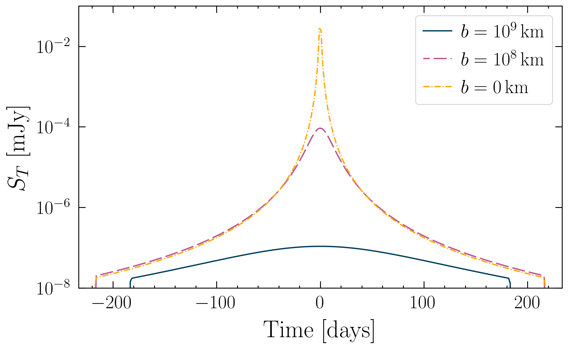
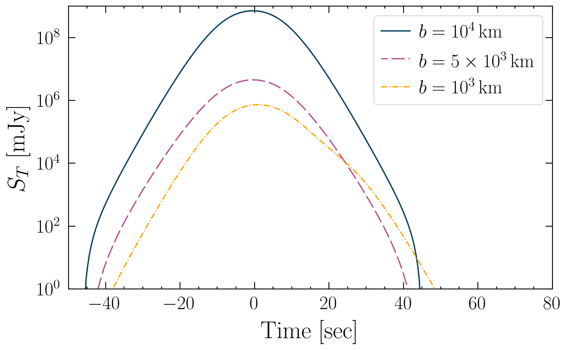
Before delving into details, let us first provide a high-level overview of the properties and characteristics of these transient events. The radio emission from an interaction of an axion clump with a neutron star can endure on timescales spanning from seconds to years, depending on the characteristic size of the axion clump. During the encounter, one expects a steady rise in the flux, followed by an extended fall (see e.g. Fig. 1 for illustrative examples33 3 Notice that the right panel of Fig. 1 illustrates a rather unintuitive scaling of flux with the impact parameter, with larger values of generating stronger signals – this effect arises as a consequence of the the internal velocity dispersion in the axion star, and is discussed in Sec. IV.), with the temporal evolution set by the density profile and the impact parameter. Notice that for typical velocities km/s, the maximum impact parameter leading to radio emission is roughly comparable to the size of the axion clump itself; for the fiducial models shown in Fig. 1, this maximum impact parameter roughly corresponds to the blue line. In addition to the long term time evolution of the signal, one expects time structure to appear at the level of the rotational period of the neutron star (spanning from seconds for a typical pulsar, which is typically much less than the transient timescale); this is a consequence of having a misalignment between the magnetic and rotational axes, and a highly asymmetric axion phase space near the neutron star. The asymmetry in the axion phase space is also expected to generate a highly inhomogeneous radio signal, especially in the case of small clumps, which may only illuminate a small fraction of the sky. Finally, it is worth highlighting that the central densities of these objects can be extremely large, meaning that they may be observable to extragalactic, or even cosmological, distances (depending on the details of the object and the axion-photon coupling). For example, consider the peak flux density produced from the axion star-neutron star encounter shown in Fig. 1: for an impact parameter of km at a distance of 1 kpc from Earth (and fixing parameters to the fiducial values shown in Table 1), we find a peak flux of mJy; assuming a telescope sensitivity of mJy (roughly consistent with the minimum flux density observed from a fast radio burst, see Petroff et al. 2016), this event could be observed out to distances of Mpc, i.e. anywhere in the Local Group.
The organization of this paper is as follows. In Sec. II we describe the current knowledge of axion miniclusters and axion stars – including their formation, properties, and evolution over the cosmic history. In Sec. III we outline the formalism used to treat the gravitational disruption of these objects, as well as photon production and propagation. Finally, we present the results of this analysis in Sec. IV, illustrating the characteristic strength of the radio signal, its anisotropy on the sky, the time-domain structure, the spectral properties, and the sensitivity of these quantities to e.g. the impact parameter and relative velocities. We conclude in Sec. V.
II Axion Miniclusters and Axion Stars
In this section, we outline the current knowledge of axion miniclusters and axion stars, motivating in particular the characteristic properties used to compute the radio signals generated in the remainder of this paper.
II.1 Axion Miniclusters
An axion minicluster is a self-gravitating virialized clump of axions Hogan and Rees 1988; Kolb and Tkachev 1993; Kolb and Tkachev 1994b; Kolb and Tkachev 1996; Zurek et al. 2007. Although axion miniclusters have been discussed for more than four decades, many of their properties are still unclear. They form from inhomogeneities in the initial axion density field and thus are mostly relevant in the post-inflationary Peccei-Quinn (PQ) symmetry breaking scenario. Numerical simulations of the axion field through the QCD phase transition Kolb and Tkachev 1994a; Vaquero et al. 2019; Buschmann et al. 2020 as well as from matter-radiation equality until redshift Eggemeier et al. 2020 have been carried out to infer the mass function as well as the density profiles of axion miniclusters. While we have learned much about miniclusters in the post-inflationary PQ scenario from these simulations, there are still many open questions. Among the properties most relevant for this work are the minicluster density profiles, which are expected to sit somewhere between a power law and a broken power law. The formation of the most massive axion miniclusters arguably involves hierarchical merging; in this case one would expect their density profile to be described by a Navarro-Frenk-White (NFW) profile Navarro et al. 1996
| (1) |
where is the characteristic density and the scale radius. On the other hand, the initial formation mechanism of axion miniclusters from the overdensities imprinted in the axion field is more akin to a direct collapse when gravity starts to be relevant around matter-radiation equality Zurek et al. 2007; O’Hare and Green 2017. In this case, the density profile should be given by a power-law Bertschinger 1985; Zurek et al. 2007
| (2) |
Assuming that the miniclusters formed from direct collapse shortly before matter radiation equality, their characteristic density is given in terms of the overdensity Kolb and Tkachev 1994b
| (3) |
where is the averaged density of axions at matter-radiation equality. Should axions comprise the entirety of the dark matter, (assuming Planck cosmology Aghanim et al. 2020b). From the simulations of the axion field through the QCD phase transition, one obtains a typical values of Buschmann et al. 2020 at matter-radiation equality. Hence, a typical value for the density scale of axion miniclusters is , although is obviously very sensitive to the value of . The density profiles of axion miniclusters in the Milky Way will also be affected by encounters with stars Dokuchaev et al. 2017; Kavanagh et al. 2021; Dandoy et al. 2022; Shen et al. 2022, although we neglect such effects here.
In order to relate the mass of the minicluster and its typical density to those of a NFW or power-law density profile we follow Refs. Fairbairn et al. 2018; Kavanagh et al. 2021. For the NFW profile, we identify
| (4) |
where and we choose a concentration parameter . We truncate the NFW profile at . For the power-law profile, we choose a truncation radius
| (5) |
and fix the normalization of the profile, Eq. (2) via .
For the velocity profile of axions in the minicluster, we assume a Maxwell-Boltzmann distribution with velocity dispersion truncated at the escape velocity ,
| (6) |
in the minicluster rest frame. In Eq. (6), denotes the Heaviside step function. The normalization coefficient is given by
| (7) |
For a virialized minicluster with spherically symmetrical density distribution , the velocity dispersion is given by the circular velocity, where Binney and Tremaine 2008
| (8) |
is the mass enclosed within the radius . Similarly, the escape velocity is given by the gravitational potential at ,
| (9) |
For the numerical results shown in this work, we consider axion miniclusters with an NFW profile. Furthermore, we neglect the radial dependence of the escape velocity and velocity dispersion, and set these quantities to their respective values evaluated at . This is done in order to simplify the sampling procedure, however it is worth emphasizing that this can be corrected in a straight-forward manner by employing an importance sampling scheme. We have validated that for the examples shown this approximation has a negligible impact on the radio flux.
II.2 Axion Star
Axion stars Kaup 1968; Ruffini and Bonazzola 1969; Tkachev 1986 are, like axion miniclusters, self-gravitating clumps of axions. However, while axion miniclusters are virialized objects formed from the direct collapse of overdensities in the axion field or hierarchical mergers of such direct-collapse miniclusters, axion stars are equilibrium solutions of the classical axion field equations found by balancing the self-gravity of the (classical) field describing an axion configuration with the gradient pressure of that field. It has been shown in numerical simulations that axion stars form efficiently in the centers of axion miniclusters Levkov et al. 2018; Eggemeier and Niemeyer 2019; Chen et al. 2021, although in what follows, for simplicity, we will treat axion stars as isolated objects.
A heuristic explanation of the properties of axions stars in the classical field description based on balancing self-gravity with the gradient pressure of the field can, e.g., be found in Ref. Visinelli et al. 2018. One can also understand the properties of an axion star heuristically in the axion particle picture: Let us denote the mass and radius of the axion star configuration as and , respectively, and the typical velocities of axions in the axion star as . The contributions of the axions’ kinetic energy and the self-gravity and to the axion star’s energy are then
| (10) |
Since the axions are confined in a volume with linear dimensions , their velocities must at least be as large as what is dictated by the uncertainty principle, , where is the axion mass.44 4 Equivalently, one can note that the size of an axion configuration with velocity must be at least as large as the axions’ De Broglie wavelength, . If one substitutes this relation into Eq. (10), one finds that the energy of the configuration is minimized for
| (11) |
In order to fit this heuristic result to numerical solutions of axions, we have here replaced with , the radius containing 90 % of the axion star’s mass, and inserted a numerical coefficient, Visinelli et al. 2018.
Beyond the characteristic mass-radius relations of axion stars, , we can learn two more lessons about axion stars from this heuristic argument: First, the gradient pressure stabilizing axion stars in the classic field picture has its origin in the particle nature of axions and the uncertainty principle; note that in the literature this gradient pressure is sometimes referred to as “quantum pressure”. Second, the heuristic argument suggests that axion stars are the densest axion configurations possible held together by gravity. While denser axion configurations are possible if they are bound by forces other than gravity, for example, the characteristic attractive quartic self-interactions of axions, such denser configurations are unstable to perturbations and/or decay quickly Schiappacasse and Hertzberg 2018; Visinelli et al. 2018. The instabilites brought about by the self-interactions also set a maximal mass for (stable) axions stars,
| (12) |
where is the axion decay constant controlling the self-interactions.
The precise density profile of axion stars can only be determined from numerical solutions to the axion equations of motion; in general, a “sech” Ansatz has been shown to yield a good fit to the numerical solutions over a wide range of masses Schiappacasse and Hertzberg 2018,
| (13) |
where . For the numerical results shown in this work, we will use axion star density profiles directly obtained from solving the equations of motions following Ref. Visinelli et al. 2018.55 5 Note that we use the “non-relativistic (single harmonic) limit” of Ref. Visinelli et al. 2018 and neglect axion self-interactions as appropriate for the “dilute” axion stars we are interested in here.
For the velocity distribution of axions in the axion star we assume a flat distribution, , truncated at the escape velocity . Note that this yields a velocity distribution compatible with the uncertainty principle giving rise to the pressure support of axion stars.
III From Gravitational Disruption to Photon Detection
In general, the radio signal generated from axion-photon mixing is obtained by integrating the coupled equations of motion for the axion and photon over the trajectories of the in-falling axions. This problem simplifies significantly by noticing that the ‘non-resonant’ mixing far from the neutron star (where ) scales with the power in the magnetic field at length scales comparable to the (inverse) momentum transfer () Marsh et al. 2022. For the axion masses we are interested in [], this non-resonant contribution is negligible in neutron star magnetospheres, instead, the mixing is strongly dominated by local resonances near the neutron star which occur when the axion 4-momentum matches that of photons, . Note that for non-relativistic particles in a strongly magnetized plasma, roughly corresponds to , where the plasma frequency , with being the electron/positron charge density, and being the mass. Focusing exclusively on the resonant contribution to the photon flux, one can express the photon production rate as
| (14) |
where is the hyper-surface defined by the manifold over which , is the normal to , is the axion phase space (normalized to the energy density)66 6 Note that we have defined using a notation that differs slightly from that of Witte et al. 2021., and is the axion-to-photon conversion probability. It is worth noting the resonant condition depends on the axion energy, the plasma frequency, and the relative angular orientation of the axion momentum with respect to the magnetic field; as a result of the angular dependence, the conversion surface is actually a fattened version of the 2-dimensional surface defined by , with the width of the fattened volume at the level of . For simplicity, in what follows we neglect this fattening of the resonance hyper-surface, treating it instead as a 2-dimensional surface defined by ; we have verified that this approximation introduces a negligible error in the calculation.
The remainder of this section is devoted to describing in detail how we solve Eq. (14), and how geometric ray tracing methods can be used to relate Eq. (14) to observable quantities such as the flux density. Our procedure relies on computing Eq. (14) via a Monte Carlo (MC) integration, and thus the description below focuses primarily on how to draw, and subsequently weight, each of the MC samples.
III.1 The Conversion Surface
Let us start by focusing on the surface integral. We will assume throughout this work that the charge density of the magnetosphere is given by the charge-separated Goldreich-Julian (GJ) distribution Goldreich and Julian 196977 7 Note that this expression neglects a relativistic factor which become important near the light cylinder . The focus here, however, is at distances , and this term is negligible.; here, is the angular velocity of the pulsar, and it is is assumed that is misaligned with respect to the magnetic field (which we assume to be purely poloidal dipolar) by an angle . Notice that definition of above is enough to uniquely describe the spatial structure of , and thus we have also uniquely set the structure of the conversion surface itself.
In order to perform the surface integral in Eq. (14), we uniformly sample the conversion surface using the procedure described in Witte et al. 2021. This allows us to re-express Eq. (14) as
| (15) |
where the summation runs over the MC samples obtained at positions , and the factor is the maximum radial distance chosen in the surface area scheme (i.e. , is chosen to be any number greater than the maximal radial distance of the conversion surface, see e.g. Witte et al. 2021). The surface normal is obtained by taking the gradient of the plasma frequency at .
Before continuing, it is worth emphasizing the charge-separated GJ model is only expected to provide a rough estimate of the plasma frequency of active pulsars (although it is in excellent agreement with the electrosphere model of dead pulsars at small radii, see e.g. Safdi et al. 2019), and as such caution should be taken in the quantitative interpretation of the results presented.
III.2 The local axion phase space distribution
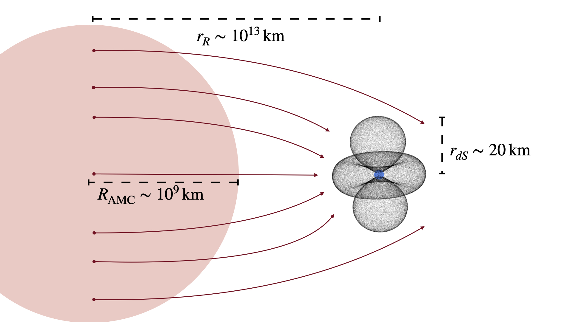
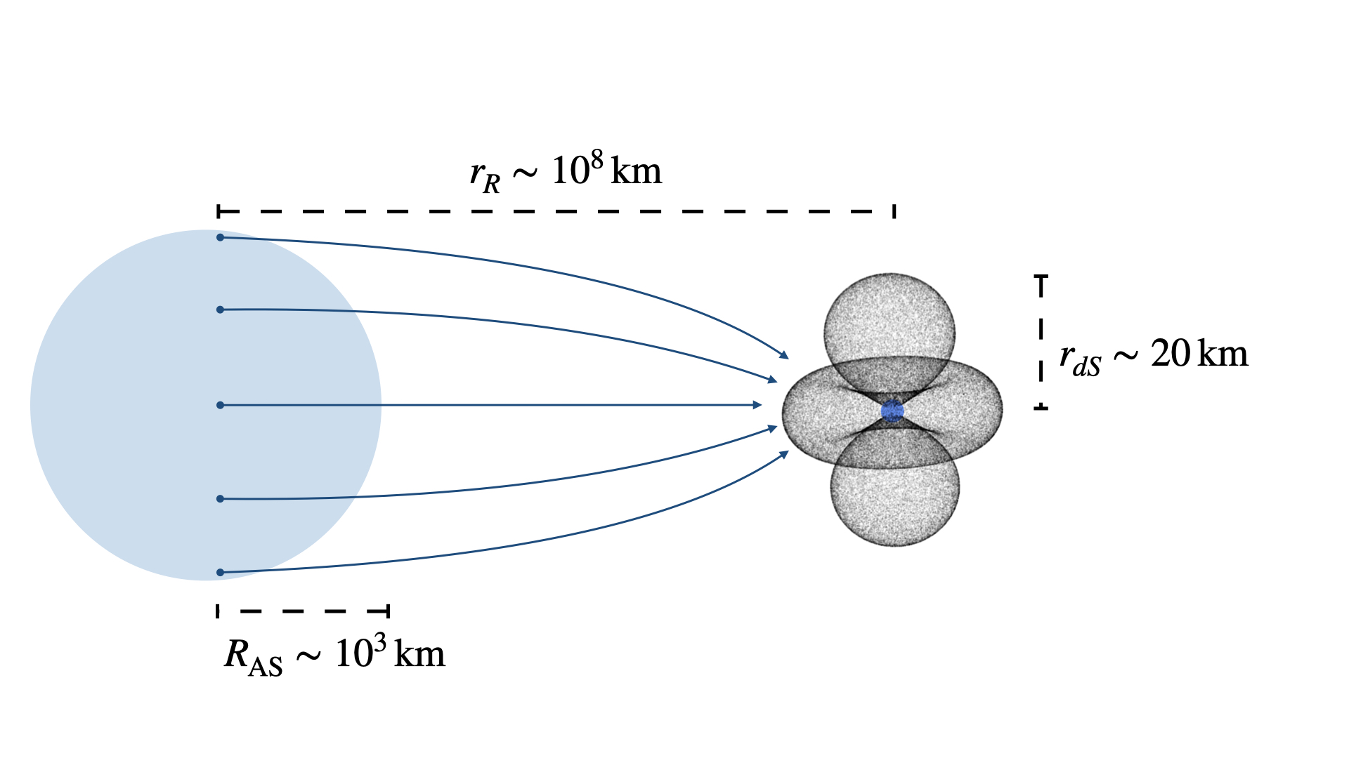
We now turn our attention to the integration over the local velocity distribution in Eq. (15), which is complicated by the fact that axion clumps falling through the magnetosphere will have their phase space ‘spaghettified’, i.e. it will become heavily concentrated along a narrow set of in-falling trajectories; this effect is illustrated (along with the characteristic scales in the problem) in Fig. 2. In order to simplify the problem, we use Liouville’s theorem to relate the local phase space density to the phase space density far away from the neutron star. For practical purposes, we choose to work under the assumption that the disruption of a minicluster or axion star can be treated as an instantaneous event occurring at the Roche radius (this is the distance at which the tidal force exerted by the neutron star exceeds the self gravity of the object itself ). This approximation implies that miniclusters and axion stars are treated as a freely propagating bodies at distances , and the axions comprising these objects are treated as independent free-falling objects at ; see e.g. Ref. Bai et al. 2022 for a justification of this approximation. Switching the integration variable to the velocity at the Roche radius , Eq. (15) can be expressed as
where is the Jacobian relating the local velocity to that at the Roche radius, and is the spatial position at the Roche radius consistent with producing a trajectory from that intersects the conversion surface at .
We can perform the velocity integral by drawing MC samples from the normalized velocity distribution at the Roche radius , where we have boosted the velocity distribution discussed in Sec. II by the relative velocity between the axion clump and the neutron star. Neglecting relativistic effects and assuming conservation of energy and angular momentum, one can relate the to the local velocity at a position via Alenazi and Gondolo 2006
| (16) |
For a fixed value of and , this equation can be inverted to solve for a maximum number of two solutions . Under this procedure, the production rate simplifies to
| (17) |
where the summation over accounts for all possible solutions to Eq. (16), and we have re-expressed the energy density in terms of the number density .
The only remaining piece is to determine the axion number density at . This can be obtained by evolving each axion trajectory backward to the Roche radius (under the assumption of Newtonian gravity). At the Roche radius, the number density can be directly evaluated for any choice of density profile and impact parameter. We note that while tracing the axion trajectory, we treat the interior of the neutron star to be at constant density88 8 Notice that if we made the point mass approximation, we could have bypassed back-tracing the axion by setting the initial velocity and distance (the later fixed to the Roche radius), and enforcing conservation of angular momentum. We have used this procedure to instead verify the accuracy of this back-tracing procedure. and take the mass and radius of the neutron star to be and km. It is worth highlighting that for maximally allowed axion-nucleon couplings, the mean free path of axions through nuclear matter is many orders of magnitude larger than the neutron star radius, and thus we need not be concerned with issues of absorption.
III.3 Photon Production
The final ingredient required to evaluate the photon production rate is the axion-photon conversion probability, which we take from Millar et al. 202199 9 This equation is derived in Ref. Millar et al. 2021 by writing down the modified version of Maxwell’s equations to include the background axion field, and looking for a plane wave solution in the WKB limit (i.e. the limit in which the axion momentum is larger than the first derivatives of the electric fields). The final expression for the ‘conversion probability’ reflects the ratio of the energy density stored in outgoing propagating Langmuir-O modes relative to the incoming axion field. :
| (18) |
Here, we have introduced the factor and defined
| (19) |
where and point in the direction parallel and perpendicular to the axion momentum, and we adopt a sign convention such that . In this work, we focus on the small coupling regime where , and employ the perturbative calculation shown in Eq. (18). Depending on the properties of the neutron star, the conversion probability can become for axion-photon couplings as small as ; in that case, the perturbative calculation is no longer correct, and the photon flux may be significantly modified – see e.g. Foster et al. 2022; Carenza and Marsh 2023 for a discussion. Importantly, this implies that the flux density estimates shown here cannot simply be re-scaled in order to estimate the sensitivity to the axion-photon coupling.
Before continuing, a comment on the conversion probability is in order. The derivation of Eq. (18) assumes that axions and photons travel on approximately straight trajectories over the “conversion length” , and that variations in the background can be approximated by a linear expansion. The second of these can be treated by either truncating the conversion length at the scale over which these assumptions fail, or by keeping higher order terms in the expansion Millar et al. 2021 – for the examples of interest, this can be treated be ensuring the conversion length stays below km scales. Photon refraction, on the other hand, can invalidate the assumption of straight trajectories on much smaller distance scales. At the moment, the extent to which this premature photon refraction modifies the conversion probability is unclear. Reference Witte et al. 2021 has proposed a procedure for truncating the conversion length when refraction becomes significant, leading to a maximally conservative estimate of the conversion probability – this technique is sometimes called the ‘-cut’, or the de-phasing cut. In what follows, we will in most cases apply the de-phasing cut so as to avoid the potential over-estimation of the radio flux (and we will clarify explicitly when this is not applied).
III.4 Photon Propagation
Until now, we have focused on computing the rate of photon production at the resonant conversion surface. In order to understand the properties of the radio flux, one must connect this rate with the distribution and properties of photons far from the neutron star. This connection can be accomplished using geometric ray tracing methods, which follow the group velocities of the sourced electromagnetic modes as as they refract and reflect off the background plasma (in what follows, we will use the term ‘photons’ to refer to the group velocities of excited electromagnetic modes); such algorithms have already proven invaluable in understanding the radio properties generated from axions near neutron stars Leroy et al. 2020; Witte et al. 2021; Battye et al. 2021; Foster et al. 2022; Noordhuis et al. 2022.
Given a dispersion relation , the ray tracing equations are
| (20) | |||||
| (21) | |||||
| (22) |
where the third equation controls the dispersive effect of the plasma, giving rise to line-broadening. For the highly magnetized environments of interest, we are interested solely in Langmuir-O (L-O) mode, as this is the only propagating mode that mixes with the axion (mode mixing is not expected to arise in these environments, see e.g. Witte et al. 2021). The dispersion relation of the L-O mode is given by
| (23) |
where is the angle between and the magnetic field.
We propagate all photons to a sphere around the neutron star with radius equal to that of the light cylinder 1010 10 Note that we choose this distance for two reasons: it is sufficiently far from the neutron star that photon trajectories are to a good approximation parallel, and the assumption of a GJ charge distribution and dipolar magnetic field breaks down. Neglecting uncertainties associated to the latter point, this choice has been shown to be robust Witte et al. 2021., bin the photons in pixelated regions on the sky of angular area , and compute the differential power via
| (24) |
where is the weight (defined by the contribution to Eq. (III.2)) of each photon, and the sum is confined to photons whose final locations are included in the pixel of interest1111 11 Here, we neglect resonant cyclotron absorption, which can induce an suppression of the flux for neutron stars with large magnetic fields (see Witte et al. 2021). . The energy is set by the sum of the asymptotic energy of the axion prior to in-fall with the energy shift due to plasma broadening, and thus naturally accounts for the redshifting of the photon as it escapes the gravitational potential.
The flux density observed by a telescope is then given by
| (25) |
where is the distance to the neutron star and is the bandwidth of the observation. The central value and characteristic width (in units of axion mass) of the spectral line in each bin can also be computed via
| (26) | |||||
| (27) |
For the examples of interest, the characteristic shift in is much less than the effect of line broadening, and thus we will assume that the spectral properties are entirely determined by the latter.
|
IV Results


In this section we present the main results of this work, answering fundamental questions needed to search for axion clump-neutron star encounters, including: what is the expected magnitude and anisotropy of the radio transients, is there significant time-domain structure, what is the width of the spectral line, and how these properties change as a function of e.g. impact parameter and relative velocity. In what follows, we adopt a fiducial set of parameters (listed in Table 1), and vary them systematically in order to understand the impact of our assumptions.
IV.1 Anisotropy of Radio Flux
Let us begin by looking at the anisotropy of the radio signal generated by a minicluster-neutron star encounter. In order to help disentangle the various effects that can contribute to the anisotropy of the flux, we begin by producing results without the de-phasing cut described in Sec. III.3 (implying the flux densities are likely overestimated).
In Fig. 3 we plot the flux density observed across the sky (as viewed by an observer situated at the center of the neutron star) for various minicluster-neutron star encounters; the panels illustrate the effect of changing the orientation between the asymptotic minicluster velocity (in the neutron star rest frame) and the neutron star rotation axis. It is worth highlighting that all sky maps generated throughout the paper represent what an observer would view at a fixed snapshot in time; for simplicity, we choose this time to align with the peak of the flux density generated throughout the encounter (see e.g. the time points in Fig. 1).




The maps presented in Fig. 3 show complex small scale structures which are not easy to explain from the intrinsic geometry of the problem. In order better under their origin, we identify the photons in the map (top panel) for which , and project these photons back onto the conversion surface. This procedure is illustrated in Fig. 4, where each photon has been colored by its relative contribution to the flux (top) or its final sky location (bottom; again, this angle is defined relative to the axis of rotation). The bright bands identified in Fig. 3 emanate from very small localized regions in the neutron star magnetosphere – it is straightforward to identify these regions as arising from ‘glancing’ axion trajectories, i.e. trajectories for which is very small (note that this roughly corresponds to axion trajectories moving perpendicular to the plasma gradient at the conversion surface). In the case of the smooth dark matter halo, the relative phase space associated with such glancing trajectories is small, and thus such features do not arise; here, however, no such suppression exists; rather, the phase space is effectively ‘spaghettified’, i.e. it is heavily concentrated along a narrow set of in-falling trajectories (note that if the asymptotic velocity distribution were a pure delta function, each point on the conversion surface would be uniquely defined by at most two velocity vectors).
In order to remain as conservative as possible in our estimates of the signal strength, we apply the de-phasing cut to all subsequent calculations. This de-phasing is driven by photon refraction, one expects a strong suppression in the conversion probability of glancing axion trajectories since the large tangential plasma gradients help drive pre-mature refraction. In order to visualize this effect, we repeat the above procedure for the same set of minicluster-neutron star encounters, but applying the de-phasing cut – the results are shown in Fig. 5 and Fig. 6. One can see that the de-phasing cut induces both a net suppression of the flux density, a significant smoothing of all small-scale features, and a relative shift in the sky location of the peak flux. The projection plots also illustrate that the brightest photons now emanate from a much broader region across the conversion surface.
Owing to the compact nature of axion stars, axion star-neutron star encounters are expected to give rise to much stronger, but also more anisotropic, signals. We illustrate the magnitude and anisotropy that can arise from such encounters in Fig. 7, where as before we have shown the results for our fiducial model parameters (including the de-phasing cut), and varied the relative orientation of the encounter from to . Notice that at its brightest, the flux density is increased by up to 11 orders of magnitude compared to that of the minicluster encounter, however, a large fraction of the sky observes effectively no radio flux.
IV.2 Time structure
We now turn our attention to the short-term time structure of the radio signal generated from the axion clump-neutron star encounters (recall that the long-term time structure, depicted in Fig. 1, is dictated by the density profile of the object prior to in-fall, whereas the short-term time structure is dictated by the rotational period of the pulsar). For typical pulsars, this amounts to looking for variation in the flux density on timescales of seconds.
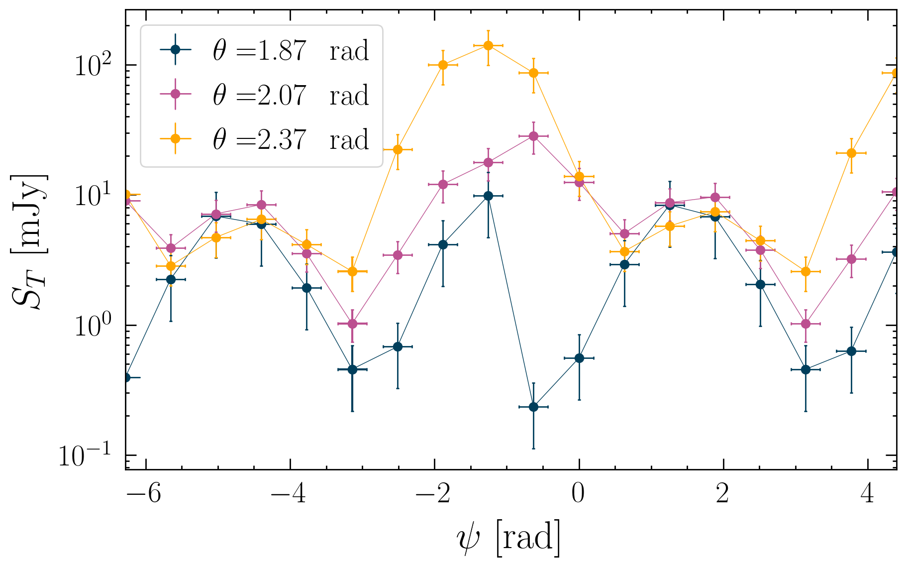
For the fiducial axion clump encounter, we generate 12 sky maps evenly spaced over the rotational period of the pulsar. We isolate a number of small regions on the sky , and compute the flux density at that point in each sky map.
The top panel of Fig. 8 illustrates the temporal behavior (as a function of rotational phase ) of a typical minicluster-neutron star encounter, where we have taken and 0.9 radians, and . The solid lines are obtained by taking an azimuthal slice through the sky map – note that this is the temporal dependence that would arise if the phase space were isotropic (as e.g. studied in Witte et al. 2021); this approach continues to serve as a good approximation so long as the asymptotic phase space is approximately homogeneous, as is the case for a minicluster. The horizontal error bars associated to each point in Fig. 8 represent the width of the azimuthal bin over which the flux is averaged. The vertical bars, on the other hand, are a rough approximation of the statistical uncertainty (and are intended to illustrate the agreement between the two procedures); these are obtained by generating 6 sky maps at (each with 5 million photons), taking 10 evenly spaced values at a fixed , and determining the average standard deviation of each sample (normalized to the mean flux). In reality, we plot to account for the fact that this uncertainty enters both the discrete data points as well as the azimuthal slice (solid curve).
In the bottom panel of Fig. 8 we show the temporal evolution of the axion star-neutron star encounter over a timescale slightly larger than the rotational period of the neutron star. In the case of the axion star, the inhomogeneity is so large that the azimuthal slice approximation is inapplicable, and thus we do not plot this quantity for comparison. Fig. 8 illustrates two important points: the signal remains strong throughout the encounter, but exhibits order-of-magnitude variations over the rotational period of the neutron star, and similarly as for miniclusters, the peak signal strength depends on the viewing angle; however, since the axion star flux is more localised, this dependency is more pronounced.
IV.3 Line Width
One of the defining features of these radio transients is the narrow spectral line, which is roughly centered about the axion mass, that arises as a result of the extremely low escape velocities of the axion clumps. The minimal value of the characteristic line width is set by the typical velocity dispersion of axions prior to in-fall; it is well known, however, that the background plasma can induce significant spectral broadening after photon production, with the amplitude of the broadening depending on the rotational frequency and the characteristic scale of the conversion surface. Given that the signal to noise ratio scales with the (assuming an observing bandwidth ), designing an optimal radio search requires understanding the characteristic line width arising from these transient events.

In general, there are two relevant effects which can serve to broaden the line. The first is a shift in the central value of the line over the course of a rotational period (any observation averaging over long observation times would thus observe a broadened line). This effect, however, is in most cases strongly subdominant to the second effect, which is a pure broadening of the line (i.e. the case in which the central value of the line does not shift, but the width grows). As a result, in what follows we neglect the former effect and define the net width to be determined by the standard deviation of the rate-weighted photon distribution in a given pixel (see Eq. (27)).

The results for the minicluster and axion star encounters are shown in Fig. 9 and Fig. 10, respectively. As before, sky maps are shown for three different values of the encounter angle . The maximum width across all maps tends to be , however some pixels produce lines that are orders of magnitude narrower than this value.


It is worth highlighting here a major difference between the scenario of axion clump-neutron star transient encounters and the case in which radio lines are sourced from a smooth background distribution of axions. In the case of the latter, the minimum line width is set by the typical energy in the rest frame of the halo , where . Here, the minimum line width is set by the velocity dispersion of the axion clump, which can be many orders of magnitude smaller. As a result, transient encounters with highly aligned or slow rotators (where plasma broadening effects are heavily reduced) can produce far narrower, and more distinctive, lines. As an example, we plot in Fig. 11 the characteristic width that would arise from a nearly aligned rotator, with radians, showing that typical values are on the order of .
IV.4 Sensitivity to Impact Parameter and Relative Velocity
Thus far, we have kept the impact parameter and the magnitude of the relative axion clump-neutron star velocity fixed. Here, we illustrate the sensitivity of the flux density to reasonable variations in these parameters.
In the case of the minicluster-neutron star encounter, we choose to plot the phase-averaged differential power as a function of viewing angle rather than the sky map, as this quantity is closer to being directly analogous to what an observer would measure (note that while this is not exactly equivalent to the period-averaged flux, Fig. 8 verifies that is a very good approximation for the typical minicluster). As an illustrative example, we plot in Fig. 12 (as well as the corresponding flux density, for the fiducial observation parameters) for the three minicluster-neutron star encounters discussed in the sections above, such that a direct comparison can be made with e.g. the sky maps of Fig. 5.
We illustrate in Fig. 13 the dependence on the impact parameter (left), and on both the impact parameter and the relative minicluster-neutron star speed (right). To a large degree, variations in the impact parameter amount to a net overall scaling of the observed flux density. The relative minicluster speed has a minimal impact for head-on collisions, while at large impact parameters (which are far more probable), slower encounter speeds lead to larger flux densities (a natural expectation of Louisville’s theorem). Importantly, both the impact parameter and the relative velocity can strongly impact the long-term time evolution of the transient event shown in Fig. 1, significantly altering both the total length of the transient signal as well as the relative time evolution.


Axion star-neutron star encounters at non-vanishing impact parameter exhibit a subtle dependence on the internal structure of the axion star, as we now discuss. A (disrupted) axion star only reaches the conversion surface if the impact parameter is sufficiently small: with a speed of km/s at the Roche radius, the relevant impact parameters are , i.e. all encounters that generate a signal are nearly head-on. For axion star-neutron star encounters, one cannot approximate the period-averaged flux using , so in Fig. 14, we show sky maps illustrating the impact of shifting the impact parameter on an axion star-neutron star encounter, with the left map showing a head-on collision and the right a skirting trajectory (i.e. a collision which nearly misses). The anisotropy in the case of the head-on collision is somewhat similar to the fiducial model shown in Fig. 7, producing a comparable flux density but in a slightly more homogeneous manner. The skirting collision, on the other hand, is notably stronger at maximum, but is more anisotropic, producing a flux over only a small fraction of the sky. That off-set trajectories can create a stronger signal than head-on collisions may be surprising, given that the mean turn radius (point of closest approach) increases monotonically with the impact parameter. To explain this result, we note that the intrinsic velocity distribution within the axion star gives a preference for a non-vanishing speed in the and directions. This is sufficient to cause axions with small impact parameters at the Roche radius to preferentially miss the resonant surface, but modestly offset axions can be more favorably oriented to pass close to the neutron star. The strength of this effect is sensitive to the detailed (and unknown) intrinsic velocity distribution. Similar behavior can be seen in the scaling of of the temporal evolution of the axion star neutron star encounter shown in Fig. 1.
Finally, Fig. 15 shows the effect of varying the relative speed and impact parameter of an axion star-neutron star encounter, with the speed taken to be km/s instead of our fiducial assumption of 100 km/s – as before, the impact parameters are taken to be (left) and km (right). The left panel shows regions of extremely high flux (exceeding at some point mJy), and increased sky coverage when compared with fiducial sky map of Fig. 7.


V Conclusions
In this work we have investigated the signatures arising from the disruption and stripping of axion miniclusters and axion stars by neutron stars; these rare encounters are capable to producing bright transient radio lines, with frequencies roughly centered about the axion mass, that endure for timescales spanning from seconds to months. Until now, there has not been a complete description of the gravitational in-fall, photon production, and photon propagation, making it difficult to estimate the strength of the signal, the spectral characteristics, beaming effects, etc. Here, we generate the first end-to-end pipeline to follow the evolution of this system, starting from the axion phase space in the asymptotic past and going to the final photon distribution in the asymptotic future. This allows us to answer for the first time: what does the radio signal from a transient axion clump-neutron star encounter actually look like?
For minicluster-neutron star encounters, we find the anisotropy of the radio flux across the sky to be significant, with our fiducial model showing variations of the flux across the sky by 4-5 orders of magnitude. Not surprisingly, for the case of axion star-neutron star encounters the anisotropy is even more pronounced, with large fractions of the sky receiving no observable flux. For rotational frequencies and misalignment angles typical of active pulsars, we find that the line width is dominated by plasma broadening effects (thus, the relative line width of the signal ranges from ); however, for aligned and slow rotators, the width of the line can many orders of magnitude less, introducing the possibility that dead neutron stars may produce more distinctive signatures.
We also characterize the long-term and short-term time evolution of both minicluster and axion star encounters, showing that miniclusters can naturally produce time variation at least at the order of magnitude level over a rotational period, while the flux from axion stars can vary by orders of magnitude on sub-second timescales. Furthermore, we show that the strength, anisotropy, and time dependence of encounters can be strongly dependent on the relative velocity and the impact parameter of the encounter itself.
In this work we do not attempt to make any statement on the transient signals arising from the broader population of axion clump-neutron star encounters; rather, we focus on developing the formalism and tools needed to characterize the properties from a particular encounter. In addition to the methods developed here, assessing the observability (and optimizing observing strategies) of axion clumps requires a more detailed understanding of the properties and distributions of the minicluster, axion star, and neutron star populations; owing to the added complexity, we reserve such a study for future work.
Nevertheless, the results shown here have demonstrated that there exists a strong sensitivity of the radio flux to the encounter parameters, which likely necessitates large encounter rates, as strong but rare events are likely to give better sensitivity to the axion-photon coupling. In future work we intend to look at the projected transient event rate arising in nearby galaxies; this will require a detailed treatment of neutron star population synthesis and an understanding of the tidal stripping and disruption of miniclusters arising from stellar encounters. Collectively, these studies will form the basis which will allow us to address the greater challenge of understanding the observability of axion clump-neutron star transient events, with a particular focus on how to develop optimized search strategies to be employed in future radio observations.
Acknowledgements.
The authors would like to thank Christoph Weniger for his participation in the initial stage of this work. SJW is supported by the European Research Council (ERC) under the European Union’s Horizon 2020 research and innovation programme (Grant agreement No. 864035 – Undark) and the Netherlands eScience Center, grant number ETEC.2019.018. The work of SB is supported by NSF grant No. PHYS-2014215, DoE HEP QuantISED award No. 100495, and the Gordon and Betty Moore Foundation Grant No. GBMF7946. AJM is supported by the European Research Council under Grant No. 742104 and by the Swedish Research Council (VR) under Dnr 2019-02337 “Detecting Axion Dark Matter In The Sky And In The Lab (AxionDM)”. Fermilab is operated by Fermi Research Alliance, LLC under Contract No. DE-AC02-07CH11359 with the United States Department of Energy. The work of DM and GS is supported by the European Research Council under Grant No. 742104 and by the Swedish Research Council (VR) under grants 2018-03641 and 2019-02337.References
- Aghanim et al. (2020a) N. Aghanim et al. (Planck), Astron. Astrophys. 641, A6 (2020a), [Erratum: Astron.Astrophys. 652, C4 (2021)], arXiv:1807.06209 [astro-ph.CO] .
- Peccei and Quinn (1977a) R. D. Peccei and H. R. Quinn, Phys. Rev. Lett. 38, 1440 (1977a).
- Peccei and Quinn (1977b) R. D. Peccei and H. R. Quinn, Phys. Rev. D 16, 1791 (1977b).
- Weinberg (1978) S. Weinberg, Phys. Rev. Lett. 40, 223 (1978).
- Wilczek (1978) F. Wilczek, Phys. Rev. Lett. 40, 279 (1978).
- Preskill et al. (1983) J. Preskill, M. B. Wise, and F. Wilczek, Phys. Lett. B 120, 127 (1983).
- Abbott and Sikivie (1983) L. Abbott and P. Sikivie, Phys. Lett. B 120, 133 (1983).
- Dine and Fischler (1983) M. Dine and W. Fischler, Phys. Lett. B 120, 137 (1983).
- Davis (1986) R. L. Davis, Phys. Lett. B 180, 225 (1986).
- Lyth (1992) D. H. Lyth, Phys. Lett. B 275, 279 (1992).
- Hogan and Rees (1988) C. J. Hogan and M. J. Rees, Phys. Lett. B 205, 228 (1988).
- Kolb and Tkachev (1993) E. W. Kolb and I. I. Tkachev, Phys. Rev. Lett. 71, 3051 (1993), arXiv:hep-ph/9303313 .
- Kolb and Tkachev (1994a) E. W. Kolb and I. I. Tkachev, Phys. Rev. D 49, 5040 (1994a), arXiv:astro-ph/9311037 .
- Kolb and Tkachev (1994b) E. W. Kolb and I. I. Tkachev, Phys. Rev. D 50, 769 (1994b), arXiv:astro-ph/9403011 .
- Kolb and Tkachev (1996) E. W. Kolb and I. I. Tkachev, Astrophys. J. Lett. 460, L25 (1996), arXiv:astro-ph/9510043 .
- Zurek et al. (2007) K. M. Zurek, C. J. Hogan, and T. R. Quinn, Phys. Rev. D 75, 043511 (2007), arXiv:astro-ph/0607341 .
- Hardy (2017) E. Hardy, JHEP 02, 046 (2017), arXiv:1609.00208 [hep-ph] .
- O’Hare and Green (2017) C. A. J. O’Hare and A. M. Green, Phys. Rev. D 95, 063017 (2017), arXiv:1701.03118 [astro-ph.CO] .
- Dokuchaev et al. (2017) V. I. Dokuchaev, Y. N. Eroshenko, and I. I. Tkachev, Soviet Journal of Experimental and Theoretical Physics 125, 434 (2017), arXiv:1710.09586 [astro-ph.GA] .
- Fairbairn et al. (2018) M. Fairbairn, D. J. E. Marsh, J. Quevillon, and S. Rozier, Phys. Rev. D 97, 083502 (2018), arXiv:1707.03310 [astro-ph.CO] .
- Vaquero et al. (2019) A. Vaquero, J. Redondo, and J. Stadler, JCAP 04, 012 (2019), arXiv:1809.09241 [astro-ph.CO] .
- Eggemeier et al. (2020) B. Eggemeier, J. Redondo, K. Dolag, J. C. Niemeyer, and A. Vaquero, Phys. Rev. Lett. 125, 041301 (2020), arXiv:1911.09417 [astro-ph.CO] .
- Buschmann et al. (2020) M. Buschmann, J. W. Foster, and B. R. Safdi, Phys. Rev. Lett. 124, 161103 (2020), arXiv:1906.00967 [astro-ph.CO] .
- Xiao et al. (2021) H. Xiao, I. Williams, and M. McQuinn, Phys. Rev. D 104, 023515 (2021), arXiv:2101.04177 [astro-ph.CO] .
- Ellis et al. (2022) D. Ellis, D. J. E. Marsh, B. Eggemeier, J. Niemeyer, J. Redondo, and K. Dolag, (2022), arXiv:2204.13187 [hep-ph] .
- Kaup (1968) D. J. Kaup, Phys. Rev. 172, 1331 (1968).
- Ruffini and Bonazzola (1969) R. Ruffini and S. Bonazzola, Phys. Rev. 187, 1767 (1969).
- Tkachev (1986) I. I. Tkachev, Sov. Astron. Lett. 12, 305 (1986).
- Seidel and Suen (1994) E. Seidel and W.-M. Suen, Phys. Rev. Lett. 72, 2516 (1994), arXiv:gr-qc/9309015 .
- Barranco and Bernal (2011) J. Barranco and A. Bernal, Phys. Rev. D 83, 043525 (2011), arXiv:1001.1769 [astro-ph.CO] .
- Levkov et al. (2018) D. G. Levkov, A. G. Panin, and I. I. Tkachev, Phys. Rev. Lett. 121, 151301 (2018), arXiv:1804.05857 [astro-ph.CO] .
- Eggemeier and Niemeyer (2019) B. Eggemeier and J. C. Niemeyer, Phys. Rev. D 100, 063528 (2019), arXiv:1906.01348 [astro-ph.CO] .
- Chen et al. (2021) J. Chen, X. Du, E. W. Lentz, D. J. E. Marsh, and J. C. Niemeyer, Phys. Rev. D 104, 083022 (2021), arXiv:2011.01333 [astro-ph.CO] .
- Braaten et al. (2016) E. Braaten, A. Mohapatra, and H. Zhang, Phys. Rev. Lett. 117, 121801 (2016), arXiv:1512.00108 [hep-ph] .
- Schiappacasse and Hertzberg (2018) E. D. Schiappacasse and M. P. Hertzberg, JCAP 01, 037 (2018), [Erratum: JCAP 03, E01 (2018)], arXiv:1710.04729 [hep-ph] .
- Visinelli et al. (2018) L. Visinelli, S. Baum, J. Redondo, K. Freese, and F. Wilczek, Phys. Lett. B 777, 64 (2018), arXiv:1710.08910 [astro-ph.CO] .
- Kavanagh et al. (2021) B. J. Kavanagh, T. D. P. Edwards, L. Visinelli, and C. Weniger, Phys. Rev. D 104, 063038 (2021), arXiv:2011.05377 [astro-ph.GA] .
- Dandoy et al. (2022) V. Dandoy, T. Schwetz, and E. Todarello, JCAP 09, 081 (2022), arXiv:2206.04619 [astro-ph.CO] .
- Shen et al. (2022) X. Shen, H. Xiao, P. F. Hopkins, and K. M. Zurek, (2022), arXiv:2207.11276 [astro-ph.GA] .
- Eggemeier et al. (2022) B. Eggemeier, C. A. J. O’Hare, G. Pierobon, J. Redondo, and Y. Y. Y. Wong, (2022), arXiv:2212.00560 [hep-ph] .
- Pshirkov and Popov (2009) M. S. Pshirkov and S. B. Popov, J. Exp. Theor. Phys. 108, 384 (2009), arXiv:0711.1264 [astro-ph] .
- Huang et al. (2018) F. P. Huang, K. Kadota, T. Sekiguchi, and H. Tashiro, Phys. Rev. D 97, 123001 (2018), arXiv:1803.08230 [hep-ph] .
- Hook et al. (2018) A. Hook, Y. Kahn, B. R. Safdi, and Z. Sun, Phys. Rev. Lett. 121, 241102 (2018), arXiv:1804.03145 [hep-ph] .
- Safdi et al. (2019) B. R. Safdi, Z. Sun, and A. Y. Chen, Phys. Rev. D 99, 123021 (2019), arXiv:1811.01020 [astro-ph.CO] .
- Battye et al. (2020) R. A. Battye, B. Garbrecht, J. I. McDonald, F. Pace, and S. Srinivasan, Phys. Rev. D 102, 023504 (2020), arXiv:1910.11907 [astro-ph.CO] .
- Leroy et al. (2020) M. Leroy, M. Chianese, T. D. P. Edwards, and C. Weniger, Phys. Rev. D 101, 123003 (2020), arXiv:1912.08815 [hep-ph] .
- Foster et al. (2020) J. W. Foster, Y. Kahn, O. Macias, Z. Sun, R. P. Eatough, V. I. Kondratiev, W. M. Peters, C. Weniger, and B. R. Safdi, Phys. Rev. Lett. 125, 171301 (2020), arXiv:2004.00011 [astro-ph.CO] .
- Witte et al. (2021) S. J. Witte, D. Noordhuis, T. D. P. Edwards, and C. Weniger, Phys. Rev. D 104, 103030 (2021), arXiv:2104.07670 [hep-ph] .
- Battye et al. (2021) R. A. Battye, B. Garbrecht, J. I. McDonald, and S. Srinivasan, JHEP 09, 105 (2021), arXiv:2104.08290 [hep-ph] .
- Millar et al. (2021) A. J. Millar, S. Baum, M. Lawson, and M. C. D. Marsh, JCAP 11, 013 (2021), arXiv:2107.07399 [hep-ph] .
- Foster et al. (2022) J. W. Foster, S. J. Witte, M. Lawson, T. Linden, V. Gajjar, C. Weniger, and B. R. Safdi, (2022), arXiv:2202.08274 [astro-ph.CO] .
- Noordhuis et al. (2022) D. Noordhuis, A. Prabhu, S. J. Witte, A. Y. Chen, F. Cruz, and C. Weniger, (2022), arXiv:2209.09917 [hep-ph] .
- Raffelt and Stodolsky (1988) G. Raffelt and L. Stodolsky, Phys. Rev. D 37, 1237 (1988).
- Prabhu (2021) A. Prabhu, Phys. Rev. D 104, 055038 (2021), arXiv:2104.14569 [hep-ph] .
- Battye et al. (2022) R. A. Battye, J. Darling, J. I. McDonald, and S. Srinivasan, Phys. Rev. D 105, L021305 (2022), arXiv:2107.01225 [astro-ph.CO] .
- Edwards et al. (2021) T. D. P. Edwards, B. J. Kavanagh, L. Visinelli, and C. Weniger, Phys. Rev. Lett. 127, 131103 (2021), arXiv:2011.05378 [hep-ph] .
- Iwazaki (2015) A. Iwazaki, Physical Review D 91, 023008 (2015).
- Buckley et al. (2021) J. H. Buckley, P. S. B. Dev, F. Ferrer, and F. P. Huang, Phys. Rev. D 103, 043015 (2021), arXiv:2004.06486 [astro-ph.HE] .
- Nurmi et al. (2021) S. Nurmi, E. D. Schiappacasse, and T. T. Yanagida, JCAP 09, 004 (2021), arXiv:2102.05680 [hep-ph] .
- Bai and Hamada (2018) Y. Bai and Y. Hamada, Phys. Lett. B 781, 187 (2018), arXiv:1709.10516 [astro-ph.HE] .
- Dietrich et al. (2019) T. Dietrich, F. Day, K. Clough, M. Coughlin, and J. Niemeyer, Monthly Notices of the Royal Astronomical Society 483, 908 (2019).
- Bai et al. (2022) Y. Bai, X. Du, and Y. Hamada, JCAP 01, 041 (2022), arXiv:2109.01222 [astro-ph.CO] .
- Kouvaris et al. (2022) C. Kouvaris, T. Liu, and K.-F. Lyu, (2022), arXiv:2202.11096 [astro-ph.HE] .
- Petroff et al. (2016) E. Petroff, E. Barr, A. Jameson, E. Keane, M. Bailes, M. Kramer, V. Morello, D. Tabbara, and W. Van Straten, arXiv preprint arXiv:1601.03547 (2016).
- Navarro et al. (1996) J. F. Navarro, C. S. Frenk, and S. D. M. White, Astrophys. J. 462, 563 (1996), arXiv:astro-ph/9508025 .
- Bertschinger (1985) E. Bertschinger, Astrophys. J. Suppl. 58, 39 (1985).
- Aghanim et al. (2020b) N. Aghanim et al. (Planck), Astron. Astrophys. 641, A6 (2020b), [Erratum: Astron.Astrophys. 652, C4 (2021)], arXiv:1807.06209 [astro-ph.CO] .
- Binney and Tremaine (2008) J. Binney and S. Tremaine, Galactic Dynamics: Second Edition (Princeton University Press, 2008).
- Marsh et al. (2022) M. C. D. Marsh, J. H. Matthews, C. Reynolds, and P. Carenza, Phys. Rev. D 105, 016013 (2022), arXiv:2107.08040 [hep-ph] .
- Goldreich and Julian (1969) P. Goldreich and W. H. Julian, The Astrophysical Journal 157, 869 (1969).
- Alenazi and Gondolo (2006) M. S. Alenazi and P. Gondolo, Phys. Rev. D 74, 083518 (2006), arXiv:astro-ph/0608390 .
- Carenza and Marsh (2023) P. Carenza and M. C. D. Marsh, (2023), arXiv:2302.02700 [hep-ph] .