Vision Transformers are Parameter-Efficient Audio-Visual Learners
Abstract
Vision transformers (ViTs) have achieved impressive results on various computer vision tasks in the last several years. In this work, we study the capability of frozen ViTs, pretrained only on visual data, to generalize to audio-visual data without finetuning any of its original parameters. To do so, we propose a latent audio-visual hybrid (LAVisH) adapter that adapts pretrained ViTs to audio-visual tasks by injecting a small number of trainable parameters into every layer of a frozen ViT. To efficiently fuse visual and audio cues, our LAVisH adapter uses a small set of latent tokens, which form an attention bottleneck, thus, eliminating the quadratic cost of standard cross-attention. Compared to the existing modality-specific audio-visual methods, our approach achieves competitive or even better performance on various audio-visual tasks while using fewer tunable parameters and without relying on costly audio pretraining or external audio encoders. Our code is available at https://genjib.github.io/project_page/LAVISH/
1 Introduction

Humans can seamlessly process audio-visual cues and use them in unison to learn associations between auditory and visual signals (e.g., the sound of barking and the visual concept of dog). In contrast, most modern computational audio-visual models av_iclr21_lee2021crossattentional; av_eccv20_avvp; eccv18_avel; av_cvpr21_av_parsing; cvpr22_ave_cmbs; cvpr22_avqa_avqa; cvpr22_ready_audio_adaptive study each of these modalities in isolation, which leads to individually-tailored modality-specific models. While such modality-specific approaches often achieve state-of-the-art results on various audio-visual benchmarks, they also have several major shortcomings. First, optimizing and training models for a specific modality (e.g., audio or video) requires significant research effort and computing power. For example, training large-scale models for audio and video requires more than 2,000 and 5,000 V100 hours respectively nips22_audioMAE; icml21_timesformer, which is not feasible for many smaller research labs. Additionally, since modern visual and audio models are becoming larger, it can be quite costly to use separate backbone networks for processing each modality. For instance, the audio-visual MBT-Large model nips21_bottleneck, built using separate audio and visual encoders, requires more than GB of GPU memory, which is only available on the costly, high-end GPU servers such as A100. Lastly, the modality-specific approaches are only trained on individual modalities and then typically combined via late fusion. As a result, such models cannot benefit from cross-modal cues in the early layers, which often leads to suboptimal performance on audio-visual tasks requiring joint audio-visual reasoning.
The recent emergence of transformer models cvpr22_omnivore; arxiv21_polyvit; arxiv22_uavm; nips21_vatt; nips21_bottleneck has propelled research in modality-agnostic architectures for multi-modal understanding. In particular, the generality of the transformer architecture iclr21_vit makes it easy to apply these models to different modalities without any modality-specific adaptations. This property is well illustrated by the fact that transformers iclr21_vit currently define state-of-the-art across many domains, including natural language processing (NLP) icml21_clip; cvpr22_swinbert; arxiv_clip4clip; iccv21_Frozen; BERT; eccv22_tip_adapter; eccv22_eclipse; eccv22_nagrani2022learning, computer vision (CV) arxiv22_omnimae; icml21_timesformer; iccv21_vivit, audio analysis interspeech21_AST; TASLP_AST; nips22_audioMAE, speech processing interspeech22_mae_ast; nips22_tvlt_textless; iclr22_avhubert. Such an architecture convergence across different domains/modalities inspired several recent works to investigate the cross-modal generalization of pretrained transformers arxiv21_universal_engines; cvpr22_vl_adapter; nips22_ST_Adapter; arxiv21_polyvit. However, most of them are either focused on language models cvpr22_vl_adapter; arxiv21_universal_engines; nips22_few_pe, or study close-domain transfer (e.g., image video) arxiv22_omnimae; cvpr22_omnivore; nips22_ST_Adapter.
In this work, we focus on the cross-modal generalization of pretrained vision transformers (ViT) iclr21_vit to the audio-visual data. Our main inspiration for this study stems from the fact that audio can be represented as a 2D spectrogram, which summarizes 1D raw audio signal into a 2D structure akin to audio images. Prior work has shown that vision architectures (e.g., CNNs icassp17_vggish; icassp20_vggsound or ViTs TASLP_AST; nips22_tvlt_textless) can be used to process such audio images. However, most prior methods use these architectures for large-scale audio representation learning. Instead of pretraining ViTs on large-scale audio data, we hypothesize that the ViTs pretrained on images can simultaneously encode representations that are useful for both images and audio, making them useful for audio-visual tasks without large-scale audio pretraining.
To investigate this hypothesis, we propose a latent audio-visual hybrid (LAVisH) adapter that directly adapts frozen ViTs, pretrained only on images, to audio-visual tasks by adding a small number of trainable parameters for audio specialization and audio-visual fusion. Such a scheme allows us to apply frozen ViTs to audio-visual data without updating the original ViT parameters but only the parameters of our proposed LAVisH modules, which we insert into every layer of a frozen ViT. For an efficient cross-modal fusion within the LAVisH module, we use a small set of latent tokens to first compress the information from all modality-specific tokens (e.g., either audio or video) and then apply cross-attention between the latent tokens and all the tokens of another modality (e.g., either video or audio). Such a scheme allows us to eliminate the quadratic cost of standard cross-attention. Furthermore, to allow information transfer between audio-to-video and, conversely, video-to-audio, we adopt a bi-directional LAVisH scheme, which enables learning a better audio-visual representation.
In our experimental section, we demonstrate that by keeping all the original ViT parameters frozen and updating only a small set of newly added parameters, the frozen ViTs, pretrained only on image data, learn to solve complex audio-visual understanding tasks requiring a joint understanding of audio and visual contents. In particular, compared to the state-of-the-art modality-specific audio-visual approaches, our method achieves competitive or even better results on the tasks of audio-visual event localization, audio-visual segmentation, and audio-visual question answering while using a smaller number of tunable parameters, and without relying on a separate pre-trained audio encoder (e.g., VGGish icassp17_vggish, AST TASLP_AST, etc.), or costly large-scale audio pretraining. We also show that our proposed latent audio-visual hybrid adapter (LAVisH) is more effective and efficient than the standard adapter schemes Adapter.
2 Related Work
Audio-Visual Understanding. Audio-visual understanding tasks focus on the audio-visual perception of objects/events/activities av_iclr21_activeContrastive; nips21_av_contrastive; cvpr21_visualvoice; iccv19_cosep; cvpr21_cyclic; av_eccv18_Owens; av_nips18_coop; av_slowfast; nips20_avcluster using both visual and audio modalities. For instance, audio-visual event localization eccv18_avel; wacv20_ave_avrb; icassp20_ave_avin; iccv19_ave_DAM; aaai20_ave_cman; eccv22_ave_DPNet; wacv23_AVE_CLIP and audio-visual video parsing av_cvpr21_av_parsing; av_eccv20_avvp; my_nips21; eccv22_joint_avvp; nips22_group_avvp require models for recognizing and localizing joint audio-visual events (e.g., a dog barking). Most existing approaches cvpr22_ave_cmbs; aaai20_ave_cman; cvpr21_ave_psp; eccv22_ave_DPNet designed for these tasks leverage pretrained modality-specific audio and visual models to extract features and combine them via ad-hoc audio-visual fusion modules. Moreover, the tasks of sound localization av_eccv18_obj_that_sound; av_cvpr18_lls; av_tpami20_lls and audio-visual segmentation eccv22_loc_avs focus on predicting the regions in the visual scenes corresponding to a sound either using bounding boxes av_eccv20_objs_vids; av_nips20_loc; eccv22_loc_ezvsl; nips22_slavc; cvpr22_loc_mix; cvpr21_loc_lvs or pixel-wise segmentations eccv22_loc_avs. Most prior sound localization methods tackle this task using self-supervised av_cvpr18_lls; eccv22_loc_ezvsl; nips22_slavc; cvpr22_loc_mix or weakly supervised eccv20_loc_MMSL approaches by learning correspondence between audio and visual patches. Instead, audio-visual segmentation methods eccv22_loc_avs rely on ground truth masks due to the requirement for precise segmentations. Furthermore, the newly introduced audio-visual question answering (AVQA) cvpr22_avqa_avqa; cvpr19_avqa_avsd; iccv21_avqa_pano_avqa task requires methods that perceive both audio and visual modalities to answer human-generated questions about the audio-visual content. Most methods designed for this task rely on modality-specific audio and vision and models, which are combined via spatial and temporal grounding modules cvpr22_avqa_avqa. Unlike these prior methods, which either require modality-specific audio/visual models or expensive pretraining, we study the capability of frozen ViTs, pretrained only on images, to generalize to audio-visual data without any prior large-scale audio-visual pretraining.
Parameter-Efficient Transfer Learning. Parameter-efficient transfer learning aims to adapt pretrained models to new tasks using few trainable parameters. Most parameter-efficient approaches can be divided into several categories: methods that introduce a small number of additional parameters acl21_hyperformer; emnlp21_power; acl21_prefix_tuning, methods that update only a sparse set of weights in the model acl21_parameter_diff_pruning; nips21_training_sparse_masks; acl22_bitfit, and methods that learn a low-rank factorization of the model’s weights Lora. Adapter Adapter is arguably the most popular parameter-efficient technique among these methods. It consists of lightweight learnable modules inserted between every pair of layers in a pretrained model. Despite their simplicity, adapters achieved impressive results on diverse tasks in both CV nips22_polyhistor; eccv22_frozen_clip; arxiv22_vit_adapter; nips17_residual_adapters; cvpr18_efficient_multi-domain; nips22_ST_Adapter and NLP nips22_lst; Adapter; Compacter; alayrac2022flamingo. However, most adapter-based approaches are designed for unimodal settings (i.e., CV, NLP, etc.), which limits their applications to multi-modal settings since they cannot share cross-modal information. Recently, several parameter-efficient approaches have been applied to multi-modal settings iclr21_parameter_av; cvpr22_vl_adapter. However, these methods require costly large-scale multimodal pre-training. Instead, we propose a latent audio-visual hybrid (LAVisH) adapter that allows us to adapt frozen ViTs, pretrained only on images, to audio-visual tasks.
3 Technical Approach
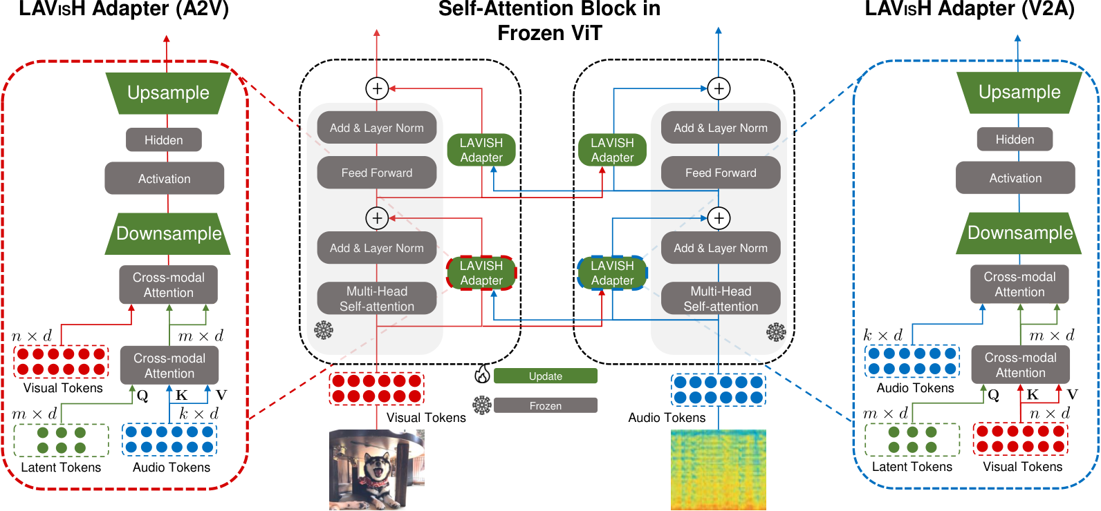
In this section, we present our proposed latent audio-visual hybrid (LAVisH) adapter that adapts frozen ViTs to audio-visual tasks by updating a small number of additional parameters. Our proposed LAVisH module, which we inject into every layer of a frozen ViT, allows the model (i) to adapt to the audio inputs and (ii) fuse information between visual and audio inputs early in the feature representation. An illustration of our method is presented in Figure 2. Below, we present our technical approach in more detail.
3.1 Audio-Visual Input Embeddings
Audio and Image Inputs. Our framework takes audio and visual inputs. For visual modality, we consider an RGB video frame with spatial dimensions sampled from a video at time . For audio, we use an audio spectrogram spanning several seconds and centered around each video frame at time .
Audio and Image Tokenization. Following the ViT iclr21_vit, we first decompose each RGB frame into non-overlapping patches and then flatten these patches into visual embeddings Similarly, we also project audio spectrograms into audio embeddings . Note that we inflate the input channel of the audio spectrogram from 1 to 3 to match the dimensions of a linear patch projection layer in the frozen ViT.
3.2 Adding LAVisH Adapters to a Frozen ViT
Next, we describe how we augment a pretrained ViT with our proposed LAVisH adapters. Every layer of a pretrained ViT in our framework consists of three main operations: (i) a multi-head attention (MHA) nips17_attention, (ii) a multi-layer perceptron (MLP), and (iii) our LAVisH adapter. As illustrated in Figure 2, we add two LAVisH adapters to every layer in the visual stream and audio stream (i.e., LAVisH adapters per layer). Note that every adapter module has its trainable parameters, i.e., the parameters in the adapter modules are not shared. Furthermore, to allow cross-modal exchange, our LAVisH adapters can transfer information from audio to visual tokens and conversely from visual to audio tokens. Such a bidirectional exchange of information ensures that both modalities aid each other in maximizing the performance of a downstream audio-visual task.
Standard ViT Layer. Before describing how to inject LAVisH adapters into a frozen ViT, we first review how a standard ViT layer processes audio and visual inputs independently. Formally, given audio and visual inputs from a layer , the standard ViT layer first independently applies MHA for the inputs from each modality:
| (1) | |||
For brevity, we skip the linear normalization layers in both MHA and MLP operations. Furthermore, for completeness, we define the MHA operation below:
| (2) |
Here, denotes an input tensor, and depict the learnable projection weights. Afterward, the intermediate representations , and obtained from the MHA layer are fed into an MLP:
| (3) | |||
The above-defined MHA and MLP operations are then repeatedly applied to audio and visual inputs in each layer of a ViT. With this formal description, we can now describe how to incorporate LAVisH adapters into a frozen ViT.
ViT Layer with a LAVisH Adapter. As mentioned above, our model consists of two types of LAVisH adapters: (i) audio-to-visual (A2V) and (ii) visual-to-audio (V2A). We first describe how to inject an A2V LAVisH adapter into a frozen ViT.
Let denote an operation that implements an audio-to-visual LAVisH adapter, which we will describe in the next subsection. Then, the updated MHA and MLP operations in each layer can be written as:
| (4) | |||
Conceptually, the operation above enables a frozen ViT to incorporate audio features into the visual representation.
Afterward, we can define a similar formulation for injecting a visual-to-audio (V2A) LAVisH adapter into a frozen ViT. Let depict an operation that implements a visual-to-audio LAVisH adapter, which we will also describe in the next subsection. Then, we can re-write the original MHA and MLP operations (i.e., Equations 1,3) for audio inputs as:
| (5) | |||
Intuitively, the operation above allows a frozen ViT to fuse information from the audio and visual tokens for a more expressive audio representation.
3.3 LAVisH Adapter
Lastly, we provide a technical description of our LAVisH adapter. In a nutshell, LAVisH adapter is a dual-pathway module that uses a small number of latent tokens to efficiently inject visual cues into the audio representation and vice-versa. It consists of four main technical components: (i) a separate set of latent tokens for audio and visual modalities, (ii) cross-modal attention between audio/visual tokens and latent tokens to compress all tokens of one modality into the latent tokens, (iii) a second cross-modal attention for efficient audio-visual fusion, (iv) a lightweight adapter module that incorporates audio-visual cues into a newly computed feature representation via a small number of trainable parameters. We now describe each of these components in more detail. A detailed illustration of our LAVisH adapter is presented in Figure 2.
Latent Tokens. Inspired by the success of several prior methods nips21_bottleneck; perceiver, we introduce a small set of randomly initialized latent audio and visual tokens , and respectively. We use a unique set of latent tokens at each layer . Here, depicts the number of latent tokens, which is significantly smaller than the total number of audio or visual tokens. For instance, the Swin cvpr22_swinv2 transformer contains audio or visual tokens. In contrast, in most cases, we use latent tokens, which is orders of magnitude smaller. The purpose of these latent tokens is to compactly summarize information from all the audio and visual tokens for efficient information transfer from one modality to another.

Cross-modal Attention. We use cross-modal attention (CMA) to implement: (i) a compression module to condense all tokens from one modality into the latent tokens of the same modality and (ii) an audio-visual fusion module, which fuses information between the compressed latent tokens of one modality and all the tokens of the other modality. We define the cross-modal attention operation as:
| (6) |
where is a learnable scalar to control the flow from one modality to another, and , , and denote query, key, and value tokens respectively.
Audio-Visual Latent Token Compression. As illustrated in Figure 2, we first use cross-modal attention to compress all the visual or audio tokens or into a small set of latent tokens or respectively. Formally, this can be written as:
| (7) | ||||
where and are the latent summary tokens for audio and visual modalities respectively. Intuitively, this operation allows us to compute latent summary tokens and as a weighted summation of all the audio or visual tokens respectively. Furthermore, because the number of latent audio and visual tokens is so small, this forces the model to include only the most relevant audio or visual information into the latent tokens. This in turn enables an efficient cross modal fusion between audio and visual tokens, which we describe next.
Audio-Visual Feature Fusion. We can use the latent summary tokens and to efficiently fuse information between audio and visual modalities. Formally, we can write this operation as:
| (8) | ||||
where depicts a newly computed audio representation that also incorporates visual cues, and similarly, denotes a new visual representation that incorporates audio cues. At a high level, both audio-visual representations and are computed as a weighted combination of the latent summary tokens and respectively. As discussed above, performing cross-modal attention between audio or visual and the latent summary tokens is beneficial because it allows us to avoid the quadratic cost of standard cross-attention operation, which would be very costly due to a large number (i.e., K) of audio/visual tokens. The resulting audio-visual representations and allow both modalities to benefit from each other when solving complex audio-visual understanding tasks.
Lightweight Adapter Module. Following prior work on adapters Adapter, we use a similar bottleneck module that consists of a learnable down-projection layer , a non-linear activation function , and a learnable up-projection layer . The entire operation can be written as:
| (9) | |||
Putting It All Together. With all the formal definitions above, we can define the final LAVisH adapter as a sequential application of the three above-described operations: (i) audio-visual latent token compression (Equation 7), (ii) audio-visual fusion (Equation 8), and (iii) the lightweight adapter module (Equation 9). Note that these operations are distinct for the visual and audio inputs. For example, the LAVisH adapter operation incorporates audio cues into the visual features whereas injects visual cues into the audio features.
4 Experimental Setup
| Method | Visual Encoder | Audio Encoder | Visual Pretrain Dataset | Audio Pretrain Dataset | Trainable Params (M) | Total Params (M) | Acc |
| AVT my_accv20_av-trans | VGG-19 ❄ | VGGish ❄ | ImageNet | AudioSet | 15.8 | 231.5 | 76.8 |
| PSP cvpr21_ave_psp | VGG-19 ❄ | VGGish ❄ | ImageNet | AudioSet | 1.7 | 217.4 | 77.8 |
| eccv22_ave_DPNet | VGG-19 | VGGish | ImageNet | AudioSet | N/A | N/A | 79.7 |
| AVEL eccv18_avel | ResNet-152 ❄ | VGGish ❄ | ImageNet | AudioSet | 3.7 | 136.0 | 74.0 |
| AVSDN my_icassp | ResNet-152 ❄ | VGGish ❄ | ImageNet | AudioSet | 8.0 | 140.3 | 75.4 |
| CMRAN acmmm20_ave_CMRAN | ResNet-152 ❄ | VGGish ❄ | ImageNet | AudioSet | 15.9 | 148.2 | 78.3 |
| MM-Pyramid acmmm22_ave_MM-Pyramid | ResNet-152 ❄ | VGGish ❄ | ImageNet | AudioSet | 44.0 | 176.3 | 77.8 |
| CMBS cvpr22_ave_cmbs | ResNet-152 ❄ | VGGish ❄ | ImageNet | AudioSet | 14.4 | 216.7 | 79.7 |
| MBT* nips21_bottleneck | ViT-B-16 | AST | ImageNet | AudioSet | 172 | 172 | 77.8 |
| MBT* nips21_bottleneck | ViT-L-16 | AST | ImageNet | AudioSet | 393 | 393 | OOM |
| LAVisH | ViT-B-16 ❄ (shared) | ImageNet | ✘ | 4.7 | 107.2 | 75.3 | |
| LAVisH | ViT-L-16 ❄ (shared) | ImageNet | ✘ | 14.5 | 340.1 | 78.1 | |
| CMBS* | Swin-V2-L ❄ | VGGish ❄ | ImageNet | AudioSet | 14.1 | 315.2 | 80.4 |
| CMBS* | Swin-V2-L | VGGish ❄ | ImageNet | AudioSet | 243.1 | 315.2 | 79.6 |
| LAVisH | Swin-V2-B ❄ (shared) | ImageNet | ✘ | 5.0 | 114.2 | 78.8 | |
| LAVisH | Swin-V2-L ❄ (shared) | ImageNet | ✘ | 10.1 | 238.8 | 81.1 | |
4.1 Downstream Tasks and Datasets
Audio-Visual Event Localization task focuses on recognizing joint audio and visual events throughout multiple time segments in a video. We evaluate on the AVE eccv18_avel dataset containing videos, where each video duration is seconds and contains events spanning categories. To adapt our approach to this task, for each time segment, we extract audio and visual features using a frozen visual transformer (e.g., ViT or Swin) augmented with LAVisH adapters. We then concatenate the audio and visual features and attach a linear layer to obtain the final audio-visual event prediction as shown in Figure 3 (a). Similar to prior approaches eccv18_avel; cvpr22_ave_cmbs; cvpr21_ave_psp; eccv22_ave_DPNet, to assess the performance of our method, we compute the fraction of correctly predicted segments and report it as our evaluation metric.
Audio-Visual Segmentation is a recently introduced task that aims to segment objects given the sound. We validate our framework on the AVSBench-S4 eccv22_loc_avs dataset, which contains videos with manually annotated pixel-wise annotations of audible objects. To adapt our framework to this task, we replace the pretrained U-Net visual encoder and the pretrained audio feature extractor of AVS eccv22_loc_avs with our frozen transformer augmented with LAVisH adapters. We then use it as our audio-visual feature extractor (See Figure 3 (b)). To evaluate our approach, we follow the evaluation protocol of AVSBench-S4, which computes the mean Intersection-over-Union (mIoU) of the predicted segmentation and the ground truth masks.
Audio-Visual Question Answering (AVQA) task requires answering questions based on the associations between objects and sounds. We conduct our experiments on the MUSIC-AVQA dataset cvpr22_avqa_avqa, which contains videos and question-answer pairs. To adapt our model to the AVQA task, we replace the pretrained visual encoder and the pretrained audio encoder of the baseline in cvpr22_avqa_avqa with our frozen transformer augmented with LAVisH adapters as presented in Figure 3 (c). Following the original AVQA work cvpr22_avqa_avqa, we evaluate our model using the answer prediction accuracy.
| Method | Visual Encoder | Audio Encoder | Visual Pretrain Dataset | Audio Pretrain Dataset | Trainable Params (M) | Total Params (M) | mIoU |
| cvpr21_loc_lvs | ResNet18 | ResNet18 | ImageNet | ✘ | N/A | N/A | 37.9 |
| eccv20_loc_MMSL | ResNet-18 | CRNN | ImageNet | AudioSet | N/A | N/A | 44.9 |
| AVS eccv22_loc_avs | PVT-V2 | VGGish ❄ | ImageNet | AudioSet | 102.4 | 174.5 | 78.7 |
| AVS* | Swin-V2-L | VGGish ❄ | ImageNet | AudioSet | 249.7 | 321.8 | 80.4 |
| LAVisH | Swin-V2-L ❄ (shared) | ImageNet | ✘ | 37.2 | 266.4 | 80.1 | |
| Method | Visual Encoder | Audio Encoder | Visual Pretrain Dataset | Audio Pretrain Dataset | Trainable Params (M) | Total Params (M) | Question | ||
| A | V | AV | |||||||
| cvpr19_avqa_avsd | VGG-19 | VGGish | ImageNet | AudioSet | N/A | N/A | 68.52 | 70.83 | 65.49 |
| iccv21_avqa_pano_avqa | Faster RCNN | VGGish | ImageNet | AudioSet | N/A | N/A | 70.73 | 72.56 | 66.64 |
| AVQA cvpr22_avqa_avqa | ResNet-18 ❄ | VGGish ❄ | ImageNet | AudioSet | 10.6 | 94.4 | 74.06 | 74.00 | 69.54 |
| AVQA* | Swin-V2-L ❄ | VGGish ❄ | ImageNet | AudioSet | 12.23 | 312.1 | 75.46 | 75.64 | 74.51 |
| AVQA* | Swin-V2-L | VGGish ❄ | ImageNet | AudioSet | 240 | 312.1 | 73.16 | 73.80 | 73.16 |
| LAVisH | Swin-V2-L ❄ (shared) | ImageNet | ✘ | 21.09 | 249.8 | 77.15 | 77.37 | 77.08 | |
5 Results and Analysis
5.1 Audio-Visual Event Localization
In Table 1, we evaluate our model on the audio-visual event localization task using the AVE eccv18_avel dataset. For our main comparisons, we focus on the recent CMBS cvpr22_ave_cmbs method, which achieves state-of-the-art results on this benchmark. For a fair comparison, we additionally implement this baseline using a Swin-V2-L cvpr22_swinv2 backbone, which is also the backbone we use in our LAVisH approach. We also include a modality-specific multimodal fusion bottleneck (MBT) baseline nips21_bottleneck with cross-modal fusion between audio and visual encoders (i.e., ViT and AST TASLP_AST) pretrained separately on large-scale image and audio datasets.
Our results in Table 1 indicate several interesting findings. First, we note that, unlike prior approaches cvpr22_ave_cmbs; eccv22_ave_DPNet; acmmm20_ave_CMRAN, our framework does not require a pretrained audio encoder or large-scale audio pretraining on AudioSet icassp17_audioset. Despite not using a pretrained audio encoder or large-scale AudioSet pretraining, our approach achieves better accuracy ( vs. ) than the state-of-the-art CMBS with the Swin-V2-L visual backbone while also requiring fewer trainable parameters (10.1M vs 14.1M). We also note that the base variant of the modality-specific dual encoder MBT nips21_bottleneck (MBT-B) achieves better performance than LAVisH with ViT-B encoder (77.8% vs 75.3%). However, the MBT approach has more trainable parameters (172M vs 4.7M). Due to the small number of trainable parameters, our approach can be scaled up much more easily than MBT. Specifically, we note that the large MBT variant (MBT-L) requires 393M trainable parameters, which leads to the out of memory issues on a 48GB A6000 GPU. In comparison, the large variant of our LAVisH approach only requires 14.5M trainable parameters, which enables memory-efficient training and inference, while also achieving higher accuracy than the best performing MBT variant (78.1% vs 77.8%). Lastly, we also observe that Swin-based variants of our model achieve consistently better accuracy than the ViT-based variants (81.1% vs 79.6%). We hypothesize that since audio information in spectrograms may be more local than in images, the locality preservation mechanism of Swin may better capture sounds with similar frequencies.
5.2 Audio-Visual Segmentation
In Table 2, we also evaluate our LAVisH approach on the audio-visual segmentation task eccv22_loc_avs on the AVSBench-S4 eccv22_loc_avs dataset. Based on our results, we first observe that our framework outperforms the previous best AVS method eccv22_loc_avs (80.1% vs 78.7%) while using fewer trainable parameters (37.2M vs. 249.7M) and without using an external audio encoder or large-scale audio pretraining. To make the comparison to the AVS baseline more thorough, we also implement it using the same Swin-V2-L backbone used by our LAVisH method. In this setting, AVS achieves similar performance to our approach (80.4% vs. 80.1%). However, this AVS variant uses significantly more trainable parameters than our method (249.7M vs. 37.2M). Thus, these results indicate that a frozen transformer augmented with our LAVisH adapters can generalize to complex dense-prediction tasks such as audio-visual segmentation.
5.3 Audio-Visual Question Answering
Finally, in Table 3, we evaluate our framework on MUSIC-AVQA cvpr22_avqa_avqa, which is an audio-visual question-answering dataset containing three categories of questions (audio, visual, and audio-visual) to assess each method’s reasoning capabilities across different modalities. We compare our LAVisH approach with the AVSD cvpr19_avqa_avsd, Pano-AVQA iccv21_avqa_pano_avqa and AVQA cvpr22_avqa_avqa methods. Like in the previous tasks, we implement a stronger AVQA baseline using a frozen Swin-V2-L backbone (i.e., the same as for our visual encoder). Based on these results, we first observe that our proposed method outperforms all prior approaches by a large margin for all three types of questions (+3.09%, +3.37%, and +7.54%). Interestingly, we notice that despite not using a pretrained audio encoder or large-scale audio pretraining, LAVisH achieves better results not only on the visual and audio-visual questions but also on the audio-based questions. This suggests that pretrained ViTs might capture representations that are useful not only for the image but also for the audio data. (i.e., audio images). We also note that LAVisH exhibits larger performance gains on audio-visual questions (+2.57%) than on visual (+1.73%) or audio-based (+1.69%). This suggests that LAVisH adapters can effectively fuse information across audio and visual modalities for the AVQA task.
| Method | Visual Encoder | Audio Encoder | Pretrain Data | Trainable Params (M) | Samples per Sec. | Acc |
| XDC nips20_avcluster | R(2+1)D | ResNet-18 | Kinetics-400 (A+V) | 45 | - | 86.8 |
| AVTS av_nips18_coop | R(2+1)D | ResNet-18 | Kinetics-400 (A+V) | 45 | - | 86.2 |
| GDT GDT | R(2+1)D | ResNet-9 | Kinetics-400 (A+V) | 39.2 | - | 89.3 |
| MBT nips21_bottleneck | ViT-B | AST-B | Kinetics-400 (V) + AudioSet (A) | 172 | 4.42 | 91.8 |
| LAVISH | ViT-B❄ (shared) | Kinetics-400 (V) | 7.4 | 6.36 | 92.6 | |
5.4 Action Recognition on UCF101.
In Table 4, we also test our model on UCF101 ucf101 action recognition. We implement LAVisH using VideoMAE codebase nips22_videomae pretrained on videos only. Compared to XDC, AVTS, and GDT, all of which used large-scale audio-visual pretraining on Kinetics-400, LAVisH achieves better results (92.6% vs. 86.8%, 86.8%, and 89.3%) with fewer trainable parameters (7.4M vs. 45M and 39.2M) and without any audio-visual pretraining. Our method also outperforms MBT, which uses ViT and AST pretrained on Kinetics and AudioSet, respectively. Overall, all the above results reveal that LAVisH is a plug-and-play module for diverse audio-visual tasks and architectures.
5.5 Ablation Studies
Next, we investigate how different design choices of our model affect the performance on the Audio-Visual Event Localization (AVE) eccv18_avel dataset.
| Method | A2V | V2A | Acc |
| AVisH | ✘ | ✘ | 77.9 |
| ✔ | ✘ | 78.7 | |
| ✘ | ✔ | 76.1 | |
| ✔ | ✔ | 79.8 | |
| LAVisH | ✘ | ✘ | 77.9 |
| ✔ | ✘ | 78.8 | |
| ✘ | ✔ | 78.7 | |
| ✔ | ✔ | 81.1 |
LAVisH Adapter Design. In Table 5, we investigate the usefulness of bidirectional cross-modal fusion and the importance of latent tokens. To do this, we first introduce an AVisH baseline that has exactly the same design/implementation as LAVisH but does not use latent tokens in its cross-attention operations. Instead, it directly performs cross-modal fusion on the original audio and visual tokens, which makes it a lot more costly than our LAVisH scheme. Furthermore, to study the importance of bidirectional cross-modal fusion, we compare our final bidirectional LAVisH approach with the unidirectional variants that only use either audio-to-visual (A2V) or visual-to-audio (V2A) cross-modal fusion, and also a baseline that does not use any cross-modal connections.
To evaluate the performance of each method, we use audio-visual event classification accuracy. Based on the results, in Table 5, we first note that the bidirectional cross-modal fusion performs better than the baseline without any cross-modal connections for both AVisH (+1.9%) and LAVisH (+3.2%) methods respectively. Additionally, we observe that the bidirectional variants of AVisH and LAVisH consistently outperform the unidirectional A2V and V2A baselines (+1.1% and +3.7% for AVisH and +2.3% and +2.4% for LAVisH ). This verifies that bidirectional cross-modal fusion enables our model better to incorporate audio and visual cues into its representation. We also investigate the importance of latent tokens by comparing LAVisH directly with AVisH. We observe that LAVisH outperforms AVisH across both unidirectional (+0.1% and +2.6%) and bidirectional variants (+1.3%). Thus, these results verify the effectiveness of both bidirectional cross-modal fusion and latent tokens.
Computational Cost Analysis. Next, we compare the efficiency of the previously described bidirectional AVisH and LAVisH methods using the GFLOPs metric. Note that because the backbone encoder is the same for both approaches, we only measure the computational cost of our introduced LAVisH modules while excluding the cost of the backbone. We observe that LAVisH is times cheaper than AVisH (11 vs. 217 GFLOPs), and LAVisH saves about GPU memory for training. This makes sense because, unlike our approach, the AVisH baseline performs cross-attention between every pair of visual and audio tokens. Due to the quadratic cost of cross-attention and a large number of tokens, this operation is very expensive. In contrast, using a small number of latent tokens (e.g., 2) enables efficient audio-visual fusion in our approach.
Comparison to Other Parameter-Efficient Schemes. In Table 6, we also compare our LAVisH adapter with other parameter-efficient methods such as Adapter Adapter, Compacter Compacter, and LoRA Lora. For each of these baselines, we follow the same training pipeline as for our LAVisH approach except that we replace our LAVisH adapters with a corresponding parameter-efficient scheme (e.g., Adapter, Compacter or LoRA). Our results suggest that LAVisH outperforms LoRA (81.1% vs. 79.1%) while also using fewer trainable parameters (10.1M vs. 17.7M). Additionally, we note that although Compacter and Adapter use fewer trainable parameters than LAVisH (10.1M vs. 8.9M and 3.7M), their accuracy is substantially lower than for our approach (81.1% vs. 79.1% and 78.4%). In sum, compared to other parameter-efficient schemes, our LAVisH adapter provides better accuracy while still being relatively parameter-efficient.
| Task | Input Modality | Accuracy | |
| AVE eccv18_avel | Vision | 75.3 | |
| Audio+Vision | 81.1 | ||
| AVS eccv22_loc_avs | Vision | 72.1 | |
| Audio+Vision | 80.1 | ||
| AVQA cvpr22_avqa_avqa | Vision | 63.2 | |
| Audio+Vision | 77.1 |
Number of Latent Tokens. Additionally, in Figure 4, we study the performance and computational cost as a function of the number of latent tokens. These results indicate that our model achieves the best accuracy with only two tokens (81.1%). Furthermore, we observe that using more latent tokens linearly increases the computational cost but does not yield better results. We conjecture that this happens because the AVE dataset is relatively small, and the model might overfit with more latent tokens. This hypothesis is supported by our results on the larger audio-visual segmentation and audio-visual question answering datasets, where the optimal number of latent tokens is 16. We note that a similar trend has also been reported in prior work nips21_bottleneck. Thus, these results suggest that LAVisH obtains a favorable trade-off between performance and efficiency as cross-modal fusion operation can be implemented very efficiently when few (i.e., 2) latent tokens are used.
Comparison with Visual-Only Baselines. To verify the importance of jointly considering audio-visual information in all three of our considered benchmarks/tasks (i.e., audio-visual event localization (AVE), audio-visual segmentation (AVS), and audio-visual question-answering (AVQA)), we compare our audio-visual approach with the visual-only variants that only consider visual information without processing any audio cues. We present these results In Table 7, and report the audio-visual variant of our approach, which jointly considers audio and visual cues, consistently outperforms the visual-only baselines by 5.8% top-1 acc., 8% mIoU, and 13.9% top-1 acc. for the AVE, AVS, and AVQA tasks respectively. These results indicate that our model benefits significantly from the joint modeling of audio and visual cues and also that visual information alone is not enough for achieving state-of-the-art results on these particular audio-visual tasks.
Comparing ViT and ResNet-152 Backbones. To investigate whether a visual transformer backbone is truly necessary for adapting a frozen visual model to an audio-visual task, we also conduct experiments with a ResNet-152 backbone resnet. We report that compared to a ViT-B iclr21_vit (86M params), using a ResNet-152 backbone (60M params) leads to a significant 18% drop in accuracy. To make the comparison fairer in terms of a model’s capacity, we also report the results using ViT-tiny (6M params) and ViT-small (23M params) architectures, which both have a smaller capacity than ResNet-152. We observe that in both of these cases, the ViT variants outperform ResNet-152 (by 5.4 % and 13.9% respectively. These results demonstrate that the lack of inductive biases in visual transformer models enables more effective transfer between inputs across different modalities.
| Method | Encoders | Visual Pretrain | Audio Pretrain | Acc |
| LAVisH | Swin-V2-L ❄ | ImageNet | ✘ | 81.1 |
| LAVisH | Swin-V2-L ❄ + VGGish ❄ | ImageNet | AudioSet | 82.4 |
| Method | Visual Encoder | Audio Encoder | Samples per Sec. | Acc |
| CMBS cvpr22_ave_cmbs | Swin-L❄ | VGGish❄ | 0.72 | 80.4 |
| LAVISH | Swin-L❄ (shared) | 1.40 | 81.1 | |
Is LAVisH Complementary to Pretrained Audio Encoders?
In Table 8, we also study whether our LAVisH approach can further benefit from audio features obtained using an external VGGish icassp17_vggish audio encoder pretrained on the large-scale AudioSet dataset. To do this, we concatenate the features from the VGGish icassp17_vggish audio encoder with the audio-visual features from our LAVisH approach and train a linear layer to predict the event category for the audio-visual event localization task. Based on the results in Table 8, we observe that using an external VGGish audio classifier leads to a boost in performance. This indicates that our LAVisH adapters and VGGish encode complementary audio information, and combining audio representations from these two sources is beneficial.
Throughput Comparisons.
In Table 9, we also compare LAVISH to CMBS [79] on the same A6000 GPU. Despite using Swin-L for audio (compared to VGGish), LAVISH has better throughput (1.40 vs. 0.72 samples/sec). This is because, unlike LAVISH, CMBS uses additional temporal modules.
6 Conclusions
In this paper, we investigate whether frozen ViTs, pretrained only on images, can generalize to audio-visual data. We demonstrate that without any audio pretraining our LAVisH adapter outperforms the state-of-the-art approaches on diverse audio-visual understanding tasks such as audio-visual event localization, audio-visual segmentation, and audio-visual question-answering. Furthermore, compared to prior approaches, our method requires a significantly smaller number of trainable parameters, enabling efficient audio-visual adaptation. In the future, we will investigate our model’s generalization ability to the audio-only and visual-language tasks, as well as the generalization of pretrained audio models to the audio-visual data.
Acknowledgments
We thank Feng Cheng, Md Mohaiminul Islam, Avinash Madasu, Maitrey Gramopadhye, and Yen-Cheng Liu for helpful discussions. This work was supported by the Sony Faculty Innovation award, ARO Award W911NF2110220, and NSF-AI Engage Institute DRL211263.
Appendix
Appendix A Implementation Details
For all of our experiments, we extract the visual frames at fps. As our best performing model, we adopt a pretrained Swin-V2-Large cvpr22_swinv2 with a spatial resolution with all parameters frozen. For the audio-visual event localization task, we implement our LAVisH adapter with latent tokens and the downsampling factor of in the 2D group convolutional adapter layers, where the number of group convolutions is set to . Our group convolution adapter layers use only 0.5x parameters as the standard fully connected ones. For the audio-visual segmentation and audio-visual question-answering tasks on AVSBench-S4 and MUSIC-AVQA, we use latent tokens and set the downsampling rate and the number of group convolutions to and , respectively. For the audio-visual action recognition on UCF101, we use the same scheme as audio-visual event localization as depicted in Figure 3 (a). We use latent tokens and set the downsampling rate and the number of group convolutions to and , respectively. For all of our experiments, we use Adam adam optimizer to train our model. We set the learning rate of LAVisH adapter to and for the final prediction layer for audio-visual event localization, for audio-visual segmentation, for LAVisH adapter and for the grounding modules and the final prediction layer in audio-visual question answering, and for audio-visual action recognition. For audio preprocessing, we compute the audio spectrogram by PyTorch pytorch kaldi fbank with triangular mel-frequency bins and frameshift in milliseconds. Then, we inflate the input channel of the audio spectrogram from 1 to 3 to match the dimensions of a linear patch projection layer in SwinV2.
| Task | Batch Size | Num. Latent Tokens | Downsampling Factor |
| AVE | 2 | 2 | 8 |
| AVS | 4 | 16 | 4 |
| AVQA | 1 | 16 | 4 |
| AVR | 2 | 24 | 4 |
References
- (1) Triantafyllos Afouras, Andrew Owens, Joon Son Chung, and Andrew Zisserman. Self-supervised learning of audio-visual objects from video. In ECCV, 2020.
- (2) Hassan Akbari, Liangzhe Yuan, Rui Qian, Wei-Hong Chuang, Shih-Fu Chang, Yin Cui, and Boqing Gong. Vatt: Transformers for multimodal self-supervised learning from raw video, audio and text. In NeurIPS, 2021.
- (3) Jean-Baptiste Alayrac, Jeff Donahue, Pauline Luc, Antoine Miech, Iain Barr, Yana Hasson, Karel Lenc, Arthur Mensch, Katie Millican, Malcolm Reynolds, et al. Flamingo: a visual language model for few-shot learning. In NeurIPS, 2022.
- (4) Humam Alwassel, Dhruv Mahajan, Bruno Korbar, Lorenzo Torresani, Bernard Ghanem, and Du Tran. Self-supervised learning by cross-modal audio-video clustering. In NeurIPS, 2020.
- (5) Relja Arandjelović and Andrew Zisserman. Objects that sound. In ECCV, 2018.
- (6) Anurag Arnab, Mostafa Dehghani, Georg Heigold, Chen Sun, Mario Lučić, and Cordelia Schmid. Vivit: A video vision transformer. In ICCV, 2021.
- (7) Alan Baade, Puyuan Peng, and David Harwath. Mae-ast: Masked autoencoding audio spectrogram transformer. In INTEERSPEECH, 2022.
- (8) Max Bain, Arsha Nagrani, Gül Varol, and Andrew Zisserman. Frozen in time: A joint video and image encoder for end-to-end retrieval. In ICCV, 2021.
- (9) Elad Ben Zaken, Yoav Goldberg, and Shauli Ravfogel. BitFit: Simple parameter-efficient fine-tuning for transformer-based masked language-models. In ACL, 2022.
- (10) Gedas Bertasius, Heng Wang, and Lorenzo Torresani. Is space-time attention all you need for video understanding? In ICML, 2021.
- (11) Honglie Chen, Weidi Xie, Triantafyllos Afouras, Arsha Nagrani, Andrea Vedaldi, and Andrew Zisserman. Localizing visual sounds the hard way. In CVPR, 2021.
- (12) Honglie Chen, Weidi Xie, Andrea Vedaldi, and Andrew Zisserman. Vggsound: A large-scale audio-visual dataset. In ICASSP, 2020.
- (13) Zhe Chen, Yuchen Duan, Wenhai Wang, Junjun He, Tong Lu, Jifeng Dai, and Yu Qiao. Vision transformer adapter for dense predictions. arXiv Preprint, 2022.
- (14) Haoyue Cheng, Zhaoyang Liu, Hang Zhou, Chen Qian, Wayne Wu, and Limin Wang. Joint-modal label denoising for weakly-supervised audio-visual video parsing. In ECCV, 2022.
- (15) Jacob Devlin, Ming-Wei Chang, Kenton Lee, and Kristina Toutanova. Bert: Pre-training of deep bidirectional transformers for language understanding. In NAACL, 2018.
- (16) Alexey Dosovitskiy, Lucas Beyer, Alexander Kolesnikov, Dirk Weissenborn, Xiaohua Zhai, Thomas Unterthiner, Mostafa Dehghani, Matthias Minderer, Georg Heigold, Sylvain Gelly, Jakob Uszkoreit, and Neil Houlsby. An image is worth 16x16 words: Transformers for image recognition at scale. In ICLR, 2021.
- (17) Ruohan Gao and Kristen Grauman. Co-separating sounds of visual objects. In ICCV, 2019.
- (18) Ruohan Gao and Kristen Grauman. Visualvoice: Audio-visual speech separation with cross-modal consistency. In CVPR, 2021.
- (19) Jort F. Gemmeke, Daniel P. W. Ellis, Dylan Freedman, Aren Jansen, Wade Lawrence, R. Channing Moore, Manoj Plakal, and Marvin Ritter. Audio set: An ontology and human-labeled dataset for audio events. In ICASSP, 2017.
- (20) Rohit Girdhar, Alaaeldin El-Nouby, Mannat Singh, Kalyan Vasudev Alwala, Armand Joulin, and Ishan Misra. Omnimae: Single model masked pretraining on images and videos. arXiv Preprint, 2022.
- (21) Rohit Girdhar, Mannat Singh, Nikhila Ravi, Laurens van der Maaten, Armand Joulin, and Ishan Misra. Omnivore: A single model for many visual modalities. In CVPR, 2022.
- (22) Yuan Gong, Yu-An Chung, and James Glass. AST: Audio Spectrogram Transformer. In INTEERSPEECH, 2021.
- (23) Yuan Gong, Yu-An Chung, and James Glass. Psla: Improving audio tagging with pretraining, sampling, labeling, and aggregation. TASLP, 2021.
- (24) Yuan Gong, Alexander H Liu, Andrew Rouditchenko, and James Glass. Uavm: A unified model for audio-visual learning. arXiv Preprint, 2022.
- (25) Demi Guo, Alexander M Rush, and Yoon Kim. Parameter-efficient transfer learning with diff pruning. In ACL, 2021.
- (26) Kaiming He, Xiangyu Zhang, Shaoqing Ren, and Jian Sun. Deep residual learning for image recognition. In CVPR, 2016.
- (27) Shawn Hershey, Sourish Chaudhuri, Daniel P. W. Ellis, Jort F. Gemmeke, Aren Jansen, Channing Moore, Manoj Plakal, Devin Platt, Rif A. Saurous, Bryan Seybold, Malcolm Slaney, Ron Weiss, and Kevin Wilson. Cnn architectures for large-scale audio classification. In ICASSP, 2017.
- (28) Neil Houlsby, Andrei Giurgiu, Stanislaw Jastrzebski, Bruna Morrone, Quentin De Laroussilhe, Andrea Gesmundo, Mona Attariyan, and Sylvain Gelly. Parameter-efficient transfer learning for nlp. In ICML, 2019.
- (29) Di Hu, Rui Qian, Minyue Jiang, Xiao Tan, Shilei Wen, Errui Ding, Weiyao Lin, and Dejing Dou. Discriminative sounding objects localization via self-supervised audiovisual matching. In NeurIPS, 2020.
- (30) Edward J Hu, Yelong Shen, Phillip Wallis, Zeyuan Allen-Zhu, Yuanzhi Li, Shean Wang, Lu Wang, and Weizhu Chen. Lora: Low-rank adaptation of large language models. In ICLR, 2022.
- (31) Xixi Hu, Ziyang Chen, and Andrew Owens. Mix and localize: Localizing sound sources in mixtures. In CVPR, 2022.
- (32) Andrew Jaegle, Felix Gimeno, Andy Brock, Oriol Vinyals, Andrew Zisserman, and Joao Carreira. Perceiver: General perception with iterative attention. In ICML, 2021.
- (33) Rabeeh Karimi Mahabadi, James Henderson, and Sebastian Ruder. Compacter: Efficient low-rank hypercomplex adapter layers. In NeurIPS, 2021.
- (34) Diederik P Kingma and Jimmy Ba. Adam: A method for stochastic optimization. In ICLR, 2015.
- (35) Bruno Korbar, Du Tran, and Lorenzo Torresani. Cooperative learning of audio and video models from self-supervised synchronization. In NeurIPS, 2018.
- (36) Jun-Tae Lee, Mihir Jain, Hyoungwoo Park, and Sungrack Yun. Cross-attentional audio-visual fusion for weakly-supervised action localization. In ICLR, 2021.
- (37) Sangho Lee, Youngjae Yu, Gunhee Kim, Thomas Breuel, Jan Kautz, and Yale Song. Parameter efficient multimodal transformers for video representation learning. In ICLR, 2021.
- (38) Brian Lester, Rami Al-Rfou, and Noah Constant. The power of scale for parameter-efficient prompt tuning. In EMNLP, 2021.
- (39) Brian Lester, Rami Al-Rfou, and Noah Constant. The power of scale for parameter-efficient prompt tuning. In EMNLP, 2021.
- (40) Guangyao Li, Yake Wei, Yapeng Tian, Chenliang Xu, Ji-Rong Wen, and Di Hu. Learning to answer questions in dynamic audio-visual scenarios. In CVPR, 2022.
- (41) Xiang Lisa Li and Percy Liang. Prefix-tuning: Optimizing continuous prompts for generation. In ACL, 2021.
- (42) Valerii Likhosherstov, Anurag Arnab, Krzysztof Choromanski, Mario Lucic, Yi Tay, Adrian Weller, and Mostafa Dehghani. Polyvit: Co-training vision transformers on images, videos and audio. arXiv Preprint, 2021.
- (43) Kevin Lin, Linjie Li, Chung-Ching Lin, Faisal Ahmed, Zhe Gan, Zicheng Liu, Yumao Lu, and Lijuan Wang. Swinbert: End-to-end transformers with sparse attention for video captioning. In CVPR, 2022.
- (44) Yan-Bo Lin, Jie Lei, Mohit Bansal, and Gedas Bertasius. Eclipse: Efficient long-range video retrieval using sight and sound. In ECCV, 2022.
- (45) Yan-Bo Lin, Yu-Jhe Li, and Yu-Chiang Frank Wang. Dual-modality seq2seq network for audio-visual event localization. In ICASSP, 2019.
- (46) Yan-Bo Lin, Hung-Yu Tseng, Hsin-Ying Lee, Yen-Yu Lin, and Ming-Hsuan Yang. Exploring cross-video and cross-modality signals for weakly-supervised audio-visual video parsing. In NeurIPS, 2021.
- (47) Yan-Bo Lin and Yu-Chiang Frank Wang. Audiovisual transformer with instance attention for audio-visual event localization. In ACCV, 2020.
- (48) Ziyi Lin, Shijie Geng, Renrui Zhang, Peng Gao, Gerard de Melo, Xiaogang Wang, Jifeng Dai, Yu Qiao, and Hongsheng Li. Frozen clip models are efficient video learners. In ECCV, 2022.
- (49) Haokun Liu, Derek Tam, Mohammed Muqeeth, Jay Mohta, Tenghao Huang, Mohit Bansal, and Colin Raffel. Few-shot parameter-efficient fine-tuning is better and cheaper than in-context learning. In NeurIPS, 2022.
- (50) Yen-Cheng Liu, Chih-Yao Ma, Junjiao Tian, Zijian He, and Zsolt Kira. Polyhistor: Parameter-efficient multi-task adaptation for dense vision tasks. In NeurIPS, 2022.
- (51) Ze Liu, Han Hu, Yutong Lin, Zhuliang Yao, Zhenda Xie, Yixuan Wei, Jia Ning, Yue Cao, Zheng Zhang, Li Dong, et al. Swin transformer v2: Scaling up capacity and resolution. In CVPR, 2022.
- (52) Kevin Lu, Aditya Grover, Pieter Abbeel, and Igor Mordatch. Pretrained transformers as universal computation engines. arXiv Preprint, 2021.
- (53) Huaishao Luo, Lei Ji, Ming Zhong, Yang Chen, Wen Lei, Nan Duan, and Tianrui Li. CLIP4Clip: An empirical study of clip for end to end video clip retrieval. arXiv Preprint, 2021.
- (54) Shuang Ma, Zhaoyang Zeng, Daniel McDuff, and Yale Song. Active contrastive learning of audio-visual video representations. In ICLR, 2021.
- (55) Shuang Ma, Zhaoyang Zeng, Daniel McDuff, and Yale Song. Contrastive learning of global and local audio-visual representations. In NeurIPS, 2021.
- (56) Rabeeh Karimi Mahabadi, Sebastian Ruder, Mostafa Dehghani, and James Henderson. Parameter-efficient multi-task fine-tuning for transformers via shared hypernetworks. In ACL, 2021.
- (57) Tanvir Mahmud and Diana Marculescu. Ave-clip: Audioclip-based multi-window temporal transformer for audio visual event localization. In WACV, 2023.
- (58) Shentong Mo and Pedro Morgado. A closer look at weakly-supervised audio-visual source localization. In NeurIPS, 2022.
- (59) Shentong Mo and Pedro Morgado. Localizing visual sounds the easy way. In ECCV, 2022.
- (60) Shentong Mo and Yapeng Tian. Multi-modal grouping network for weakly-supervised audio-visual video parsing. In NeurIPS, 2022.
- (61) Arsha Nagrani, Paul Hongsuck Seo, Bryan Seybold, Anja Hauth, Santiago Manen, Chen Sun, and Cordelia Schmid. Learning audio-video modalities from image captions. In ECCV, 2022.
- (62) Arsha Nagrani, Shan Yang, Anurag Arnab, Aren Jansen, Cordelia Schmid, and Chen Sun. Attention bottlenecks for multimodal fusion. In NeurIPS, 2021.
- (63) Andrew Owens and Alexei A. Efros. Audio-visual scene analysis with self-supervised multisensory features. In ECCV, 2018.
- (64) Junting Pan, Ziyi Lin, Xiatian Zhu, Jing Shao, and Hongsheng Li. St-adapter: Parameter-efficient image-to-video transfer learning for action recognition. In NeurIPS, 2022.
- (65) Adam Paszke, Sam Gross, Francisco Massa, Adam Lerer, James Bradbury, Gregory Chanan, Trevor Killeen, Zeming Lin, Natalia Gimelshein, Luca Antiga, et al. Pytorch: An imperative style, high-performance deep learning library. In NeurIPS, 2019.
- (66) Mandela Patrick, Yuki M Asano, Polina Kuznetsova, Ruth Fong, Joao F Henriques, Geoffrey Zweig, and Andrea Vedaldi. On compositions of transformations in contrastive self-supervised learning. In ICCV, 2021.
- (67) Rui Qian, Di Hu, Heinrich Dinkel, Mengyue Wu, Ning Xu, and Weiyao Lin. Multiple sound sources localization from coarse to fine. In ECCV, 2020.
- (68) Alec Radford, Jong Wook Kim, Chris Hallacy, Aditya Ramesh, Gabriel Goh, Sandhini Agarwal, Girish Sastry, Amanda Askell, Pamela Mishkin, Jack Clark, et al. Learning transferable visual models from natural language supervision. In ICML, 2021.
- (69) Janani Ramaswamy. What makes the sound?: A dual-modality interacting network for audio-visual event localization. In ICASSP, 2020.
- (70) Janani Ramaswamy and Sukhendu Das. See the sound, hear the pixels. In WACV, 2020.
- (71) Varshanth Rao, Md Ibrahim Khalil, Haoda Li, Peng Dai, and Juwei Lu. Dual perspective network for audio-visual event localization. In ECCV, 2022.
- (72) Sylvestre-Alvise Rebuffi, Hakan Bilen, and Andrea Vedaldi. Learning multiple visual domains with residual adapters. In NeurIPS, 2017.
- (73) Sylvestre-Alvise Rebuffi, Hakan Bilen, and Andrea Vedaldi. Efficient parametrization of multi-domain deep neural networks. In CVPR, 2018.
- (74) Idan Schwartz, Alexander G Schwing, and Tamir Hazan. A simple baseline for audio-visual scene-aware dialog. In CVPR, 2019.
- (75) Arda Senocak, Tae-Hyun Oh, Junsik Kim, Ming-Hsuan Yang, and In So Kweon. Learning to localize sound source in visual scenes. In CVPR, 2018.
- (76) Arda Senocak, Tae-Hyun Oh, Junsik Kim, Ming-Hsuan Yang, and In-So Kweon. Learning to localize sound sources in visual scenes: Analysis and applications. TPAMI, 2019.
- (77) Bowen Shi, Wei-Ning Hsu, Kushal Lakhotia, and Abdelrahman Mohamed. Learning audio-visual speech representation by masked multimodal cluster prediction. In ICLR, 2022.
- (78) Khurram Soomro, Amir Roshan Zamir, and Mubarak Shah. Ucf101: A dataset of 101 human actions classes from videos in the wild. arXiv Preprint, 2012.
- (79) Yi-Lin Sung, Jaemin Cho, and Mohit Bansal. Lst: Ladder side-tuning for parameter and memory efficient transfer learning. In NeurIPS, 2022.
- (80) Yi-Lin Sung, Jaemin Cho, and Mohit Bansal. Vl-adapter: Parameter-efficient transfer learning for vision-and-language tasks. In CVPR, 2022.
- (81) Yi-Lin Sung, Varun Nair, and Colin A Raffel. Training neural networks with fixed sparse masks. In NeurIPS, 2021.
- (82) Zineng Tang, Jaemin Cho, Yixin Nie, and Mohit Bansal. Tvlt: Textless vision-language transformer. In NeurIPS, 2022.
- (83) Yapeng Tian, Di Hu, and Chenliang Xu. Cyclic co-learning of sounding object visual grounding and sound separation. In CVPR, 2021.
- (84) Yapeng Tian, Dingzeyu Li, and Chenliang Xu. Unified multisensory perception: Weakly-supervised audio-visual video parsing. In ECCV, 2020.
- (85) Yapeng Tian, Jing Shi, Bochen Li, Zhiyao Duan, and Chenliang Xu. Audio-visual event localization in unconstrained videos. In ECCV, 2018.
- (86) Zhan Tong, Yibing Song, Jue Wang, and Limin Wang. VideoMAE: Masked autoencoders are data-efficient learners for self-supervised video pre-training. In NeurIPS, 2022.
- (87) Ashish Vaswani, Noam Shazeer, Niki Parmar, Jakob Uszkoreit, Llion Jones, Aidan N Gomez, Łukasz Kaiser, and Illia Polosukhin. Attention is all you need. In NeurIPS, 2017.
- (88) Yu Wu and Yi Yang. Exploring heterogeneous clues for weakly-supervised audio-visual video parsing. In CVPR, 2021.
- (89) Yu Wu, Linchao Zhu, Yan Yan, and Yi Yang. Dual attention matching for audio-visual event localization. In ICCV, 2019.
- (90) Yan Xia and Zhou Zhao. Cross-modal background suppression for audio-visual event localization. In CVPR, 2022.
- (91) Fanyi Xiao, Yong Jae Lee, Kristen Grauman, Jitendra Malik, and Christoph Feichtenhofer. Audiovisual slowfast networks for video recognition. arXiv Preprint, 2020.
- (92) Hu Xu, Juncheng Li, Alexei Baevski, Michael Auli, Wojciech Galuba, Florian Metze, Christoph Feichtenhofer, et al. Masked autoencoders that listen. In NeurIPS, 2022.
- (93) Haoming Xu, Runhao Zeng, Qingyao Wu, Mingkui Tan, and Chuang Gan. Cross-modal relation-aware networks for audio-visual event localization. In ACM MM, 2020.
- (94) Hanyu Xuan, Zhenyu Zhang, Shuo Chen, Jian Yang, and Yan Yan. Cross-modal attention network for temporal inconsistent audio-visual event localization. In AAAI, 2020.
- (95) Jiashuo Yu, Ying Cheng, Rui-Wei Zhao, Rui Feng, and Yuejie Zhang. Mm-pyramid: multimodal pyramid attentional network for audio-visual event localization and video parsing. In ACM MM, 2022.
- (96) Heeseung Yun, Youngjae Yu, Wonsuk Yang, Kangil Lee, and Gunhee Kim. Pano-avqa: Grounded audio-visual question answering on 360deg videos. In ICCV, 2021.
- (97) Renrui Zhang, Rongyao Fang, Peng Gao, Wei Zhang, Kunchang Li, Jifeng Dai, Yu Qiao, and Hongsheng Li. Tip-adapter: Training-free clip-adapter for better vision-language modeling. In arXiv Preprint, 2022.
- (98) Yunhua Zhang, Hazel Doughty, Ling Shao, and Cees GM Snoek. Audio-adaptive activity recognition across video domains. In CVPR, 2022.
- (99) Jinxing Zhou, Jianyuan Wang, Jiayi Zhang, Weixuan Sun, Jing Zhang, Stan Birchfield, Dan Guo, Lingpeng Kong, Meng Wang, and Yiran Zhong. Audio–visual segmentation. In ECCV, 2022.
- (100) Jinxing Zhou, Liang Zheng, Yiran Zhong, Shijie Hao, and Meng Wang. Positive sample propagation along the audio-visual event line. In CVPR, 2021.