New Covariant Feynman Rules for Effective Field Theories

We work in Lorentzian signature. Consider the background-field dependent Feynman propagator for a scalar field in an irreducible representation of the gauge and (if present) global symmetry group:

$$G_{s}(m,X)=\frac{-i}{D^{2}+m^{2}+X-i\epsilon}\,.$$

(1)

The mass $m$ is field-independent and proportional to the identity, it may be zero. In contrast, the mass $X$ is field dependent, but, since we consider irreducible representations, $X$ does not mix different representations. Representation-mixing field dependent masses will be treated as mass insertions (bilinear vertices). The gauge fixing procedure may generate contribution to $X$, see eq. (50). In the following, we will suppress the $i\epsilon$ terms.

The heat kernel (HK) representation of the propagator is defined as Fock:1937dy; Nambu:1950rs; schwinger1951

$$G_{s}(m,X)=\int_{0}^{\infty}dt\ K_{s}(t,m,X)\,,\qquad K_{s}(t,m,X)\equiv e^{-i(D^{2}+m^{2}+X)t}\,.$$

(2)

The HK $K_{s}(t,m,X)$ satisfies the Schrödinger equation³³ 3 The name ”heat kernel” originates from the Euclidean analogue which satisfies the heat equation.

$$i\partial_{t}K_{s}(t,m,X)=(D^{2}+m^{2}+X)K_{s}(t,m,X)\,,\qquad K_{s}(0,m,X)=1\,.$$

(3)

Notice that for the case of a scalar, $X$ is Hermitian. However, for nonzero spin (see below), there is a contribution to the effective mass matrix given by the term $-S^{\mu\nu}F_{\mu\nu}$, where $S_{\mu\nu}$ are the generators for Lorentz transformations which are non-Hermitian in non-Euclidean spacetime signature.

Defining $K_{s}(t,m,X;x,y)\equiv\braket{x|K_{s}(t,m,X)|y}$, one now makes the ansatz

$$K_{s}(t,m,X;x,y)=K_{0}(t,m;x-y){B(t,X;x,y)}\,,$$

(4)

where

$$K_{0}(t,m;x-y)\equiv\int\frac{d^{d}k}{(4\pi)^{d}}e^{i(k^{2}-m^{2})t}e^{-ik(x-y)}=i(4\pi it)^{-\frac{d}{2}}e^{-i\frac{(x-y)^{2}}{4t}-im^{2}t}\,,$$

(5)

is the free HK (that is, the HK of a gauge singlet with vanishing $X$). The function $B(t)$ has a regular expansion around $t=0$:

$$B(t,X;x,y)\equiv\sum_{n\geq 0}b_{2n}(X;x,y)\frac{t^{n}}{n!}\,.$$

(6)

The $b_{2n}$ are known as the heat kernel coefficients. In particular, the coefficient $b_{0}$, which is independent of $X$, is equal to the Wilson line along the straight line segment connecting $x$ to $y$ (see app. B). The higher coefficients have no closed-form expressions, however all we will need are their various covariant derivatives evaluated at coinciding arguments ($x=y$), which we will refer to as the local heat kernel coefficients (LHKC’s). These objects are local polynomials in the background fields and can be computed systematically dewitt1965dynamical; DeWitt:1967ub; Gilkey:1975iq; Avramidi:1990je; Vassilevich:2003xt. If the field transforms in the $r$ representation, $B$ transforms as the $r$ representation at $x$ (that is, from the left) and as the conjugate $\bar{r}$ representation at $y$ (from the right), since $G^{\alpha}_{\ \beta}(x,y)=\braket{\Phi^{\alpha}(x)\Phi_{\beta}^{\dagger}(y)}$. $K_{0}$ transforms as a singlet. We will be using the HK in a ”mixed position-momentum representation”

$$K_{s}(t,m,X;x,y)=\int\frac{d^{d}k}{(2\pi)^{d}}\,e^{-ik(x-y)}\biggl(e^{i(k^{2}-m^{2})t}B(t,X;x,y)\biggr)\,.$$

(7)

Sometimes an interaction contains a covariant derivative acting on a fluctuation field (this happens, for instance, in a gauge theory with scalars, see app. A). We will associate this derivative to the propagator directly, that is we also will need propagators

$$\braket{D_{\mu}\Phi(x)\Phi^{\dagger}(y)}=D^{x}_{\mu}G_{s}(m,X;x,y)\,,$$

(8)

and similar terms with a derivative acting on $y$ as well as both arguments. Such terms are easy to deal with in our formalism as $D_{\mu}G_{s}=\int dt\ D_{\mu}K_{s}(t)$, and

$$D_{\mu}^{x}K_{s}(t,m,X;x,y)=\int\frac{d^{d}k}{(2\pi)^{d}}\,e^{-ik(x-y)}\biggl(e^{i(k^{2}-m^{2})t}(-ik_{\mu}+D_{\mu}^{x})B(t,X;x,y)\biggr)\,,$$

(9)

etc.

One may evaluate explicitly the integral over the Schwinger parameter $t$ to obtain the propagator in terms of the HK coefficients:

$$G_{s}(m,X;x,y)=\int\frac{d^{d}k}{(2\pi)^{d}}\,e^{-ik(x-y)}\left(\sum_{n=0}^{\infty}\left(\frac{i}{k^{2}-m^{2}}\right)^{n+1}b_{2n}(X;x,y)\right)\,.$$

(10)

Even though the Feynman rules can be given equally well in terms of this propagator instead of the HK, we find it more practical to perform the integration over the Schwinger parameters last (in particular, after the momentum integration), so eq. (10) is not relevant for us in practice. There is however one important observation that can be made from eq. (10). Suppose $X$ is non-Hermitian, which, as we already mentioned, can occur for fields of nonzero spin. The representation of the propagator in terms of the HK in eq. (2) is not well defined for arbitrary complex eigenvalues. However, all we are interested in is the local part of the effective action, which is implied in the small-$t$ expansion of eq. (6). If we define our propagators in terms of this expanded HK, we obtain the well defined object in eq. (10).

We start by writing the fermion propagator in terms of the scalar one: ⁴⁴ 4 In the presence of a field dependent mass $Y+i\gamma_{5}Z$, we can instead write $$G(m,Y,Z)=i\left(i\not{D}-m-Y-i\gamma_{5}Z\right)^{-1}=(-i)(i\not{D}+m+Y-i\gamma_{5}Z)\left(D^{2}+m^{2}+X\right)^{-1}$$ (11) with $X=-S^{\mu\nu}F_{\mu\nu}-i\not{D}Y-\gamma_{5}\not{D}Z+2mY+Y^{2}+Z^{2}$. In most applications $Y=Z=0$.

$$G_{\!f}(m)=\frac{i}{i\not{D}-m}=(i\not{D}+m)\frac{-i}{D^{2}+m^{2}+X_{\!f}}\,,\qquad X_{\!f}\equiv-S^{\mu\nu}F^{a}_{\mu\nu}\mathfrak{t}^{a}\,,$$

(12)

where $S^{\mu\nu}=\frac{i}{4}[\gamma^{\mu},\gamma^{\nu}]$ is the Lorentz generator for spin $\frac{1}{2}$. We then define the corresponding HK

$$K_{\!f}(t,m)\equiv(i\not{D}+m)e^{-i(D^{2}+m^{2}+X_{\!f})t}\,,$$

(13)

such that as previously $G_{\!f}=\int dt\,K_{\!f}(t)$. The HK in its mixed representation that we will be using in our Feynman rules is thus

$$K_{\!f}(t,m;x,y)=\int\frac{d^{d}k}{(2\pi)^{d}}e^{-ik(x-y)}\biggl(e^{i(k^{2}-m^{2})t}(\not{k}+m+i\not{D}^{x})B(t,X_{\!f};x,y)\biggr)\,.$$

(14)

We notice that the same function $B$ appears on the right hand side, albeit with a different argument $X$.

Finally, consider the gauge sector. It is easiest to use Feynman gauge $\xi=1$ to avoid dealing with non-minimal operators.⁵⁵ 5 See ref. Barvinsky:1985an for the HK with non-minimal operators. Then from the terms quadratic in the fluctuations detailed in app. A one can read off the propagator

$$G_{v}=\frac{+i}{D^{2}+X_{v}-i\epsilon}\,,\qquad(X_{v})^{a\,\mu}_{\ b\,\nu}\equiv-2f^{a}_{\ bc}F^{c\,\mu}_{\ \ \nu}+g^{2}\phi^{\dagger}\{\mathfrak{t}^{a},\mathfrak{t}_{b}\}\phi\delta^{\mu}_{\ \nu}\,.$$

(15)

Like in the spin-$\frac{1}{2}$ case, the term in $X_{v}$ proportional to the field strength can be understood as $-S^{\mu\nu}F^{a}_{\mu\nu}\mathfrak{t}^{a}$, with the spin-1 Lorentz generator $(S^{\mu\nu})_{\alpha\beta}=i(\delta^{\mu}_{\alpha}\delta^{\nu}_{\beta}-\delta^{\mu}_{\beta}\delta^{\nu}_{\alpha})$ and the adjoint generator $(\mathfrak{t}^{a})^{b}_{\ c}=-if^{ab}_{\ \ c}$. The gauge HK can be decomposed as

$$K_{v}(t;x,y)=\int\frac{d^{d}k}{(2\pi)^{d}}\,e^{-ik(x-y)}\biggl(-e^{i(k^{2}-m^{2})t}B(t,X_{v};x,y)\biggr)\,.$$

(16)

The gauge and Lorentz indices on $G_{v}$, $K_{v}$ and $B$ are suppressed here for clarity. Notice that in the limit of vanishing background fields we obtain $B^{a\,\mu}_{\ \ b\,\nu}=\delta^{a}_{b}\delta^{\mu}_{\nu}$, recovering the usual propagator in the Feynman gauge, including the correct negative sign.

The HK for the ghost is given by the scalar one, with the field dependent mass

$$(X_{g})^{a}_{\ b}=g^{2}\,\phi^{\dagger}\{\mathfrak{t}^{a},\mathfrak{t}_{b}\}\phi\,,$$

(17)

that is of the same structure as the one for the gauge fields.

Let us first give a concise list of rules which can be directly applied to any given problem. We will provide a proof for these rules in sec. 3.2.

1. 1.

   Draw all diagrams with with no external legs.

2. 2.

   For each propagator write the expressions given in tab. 1. For propagators of derivatives of fields add additional factors of $(-ik_{\mu}+D_{\mu}^{x})$ and $(ik_{\mu}+D_{\mu}^{y})$ as explained in eq. (9). The expressions for the fermion propagator and the derivative scalar propagator assumes that the momentum $k$ flows parallel to particle-number.

3. 3.

   Write the field dependent couplings, including the usual factor of $i$ for each of them.

4. 4.

   To each vertex, associate an ingoing momentum $p_{i}$, and impose momentum conservation at every vertex. Perform the loop momentum integration in $d$ dimensions.

5. 5.

   Expand in the external momenta $p_{i}$ to the desired order, replace the momenta $p^{i}$ by the partial derivatives

   $$p_{\mu}^{i}\to i\frac{\partial}{\partial x_{\mu}^{i}}$$

   (18)

   and take the limits $x_{i}\to x$ everywhere.

6. 6.

   Integrate over the Schwinger parameters, remove all poles via $\overline{MS}$, and take the limit $d\to 4$. The result, multiplied by $-i$, is the EFT matching contribution to the Lagrangian.

If there is a field dependent mass that does not mix representations (i.e., that commutes with the field-independent mass matrix), one may wish to include it into the propagators and heat kernels. Field dependent masses that do mix representations need to be included as mass insertions (bilinear vertices).

The partial derivatives appearing in step 5 always act on a total gauge singlet, essentially the product of all the $B$-factors and field-dependent couplings (see sec. 3.2). Once these derivatives are distributed over the individual (non gauge singlet) factors, covariant derivatives will reappear.

Observe the presence of the coincidence limits $x_{i}\to x$ in step 5. This means that, as claimed in section 2, only the LHKCs, i.e., the coincidence limits of coefficients $b_{2n}$ (and their covariant derivatives) appear. A technical simplification that we already would like to point out is that any string of partial derivatives resulting from the expansion in external momenta is automatically symmetric (since partial derivatives commute)

$$\partial_{\mu_{1}}\partial_{\mu_{2}}\dots\partial_{\mu_{n}}=\partial_{(\mu_{1}}\partial_{\mu_{2}}\dots\partial_{\mu_{n})}$$

(19)

where the parenthesis on the index denotes symmetrization with strength one. This symmetrization will thus appear also in the resulting covariant derivatives, which greatly simplifies the calculation. For instance, symmetrized covariant derivatives of the ubiquitous coefficient $b_{0}$ are zero, see app. B.

A last comment concerns one-loop diagrams with zero vertices, that is with one single massive particle in the loop. This case is somewhat special since it involves the log of the propagator, but is also the most studied one in the literature Vassilevich:2003xt. For bosons one needs the functional trace identity

$$\operatorname{Tr}\log(D^{2}+X+m^{2})=-\int_{0}^{\infty}\frac{dt}{t}\operatorname{Tr}e^{-i(D^{2}+X+m^{2})t}$$

(20)

and for Dirac fermions

$$\operatorname{Tr}\log(i\not{D}-m)=-\frac{1}{2}\int_{0}^{\infty}\frac{dt}{t}\operatorname{Tr}e^{-i(D^{2}-F_{\mu\nu}S^{\mu\nu}+m^{2})t}$$

(21)

These traces are straightforwardly evaluated in terms of traces over the HK coefficients $b_{2n}(x,x)$.

We now proceed to prove the rules given in sec. 3.1.

Rule 1 just states that we are calculating the effective action in the background field method. Lines correspond to propagators of fluctuations and not to background fields, which are hidden in the lines and vertices.

Rule 2 is evident from the HK representation of the propagators $G=\int dtK(t)$ and the explicit expressions for the HK in eq. (7) and eq. (14). Notice that we are not writing the factors of $e^{ikx}$, they will be combined into momentum conserving delta functions similar to the standard (non-covariant) Feynman rules (see below). We also delay the integrations over the momenta and Schwinger parameters.

Rule 3 is self-evident.

To show rules 4 and 5, let us examine the possible spacetime dependence for a given vertex at $x$ resulting from the rules so far. For instance, consider a bilinear interaction

$$\mathcal{L}_{\rm int}=C_{\alpha\beta}(x)\Phi^{\alpha}(x)\Psi^{\beta}(x)\,,$$

(22)

where $\Phi$ and $\Psi$ are two fluctuation fields (of possibly different spins), and $C$ is a background-field dependent coupling. We suppress possible Lorentz indices and only display the gauge indices $\alpha$ and $\beta$, belonging in general to different irreducible representations. Such an interaction will give rise to factors of the kind

$$iC_{\alpha\beta}(x)B^{\alpha,\,\cdot\,}(t;x,\,\cdot\,)B^{\beta,\,\cdot\,}(t^{\prime};x,\,\cdot\,)\,.$$

(23)

This expression is gauge invariant at $x$, the gauge indices $\alpha,\beta$ are contracted in a gauge-invariant way in the same way as in the Lagrangian. For this reason, the product of all propagator $B$ factors and couplings $C$ becomes a complete gauge singlet that we call

$$\Gamma(t_{1},\dots t_{P},x_{1},\dots x_{V})\equiv\prod_{i=1}^{P}B_{i}(t_{i})\prod_{\ell=1}^{V}iC_{\ell}\,,$$

(24)

where $P$ denotes the number of propagators and $V$ the number of vertices. Diagrams with only scalar propagators become (suppressing the $t_{i}$ integrations for clarity)

$$\int\prod_{i=1}^{P}\frac{d^{d}k_{i}}{(2\pi)^{d}}e^{i(k_{i}^{2}-m_{i}^{2})t_{i}}\prod_{\ell=1}^{V}d^{d}p_{\ell}\delta(p_{\ell}-P_{\ell})\tilde{\Gamma}(t_{1},\dots t_{P},p_{1},\dots p_{V})\,,$$

(25)

where $P_{\ell}$ is the total momentum exiting at the $\ell^{th}$ vertex in the propagators. We have Fourier-transformed the ”$n$-point function” $\Gamma$ and performed the integration over the $x_{i}$ to generate momentum-conserving $\delta$ functions.⁶⁶ 6 Our convention is that factors of $e^{ikx}$ ($e^{-ikx}$) correspond to momentum $k$ exiting (entering) the vertex at $x$. This Fourier transform of $\Gamma$ introduces $V$ new ”external” ingoing momenta $p_{\ell}$, one for each vertex. The generalization to fermion propagators and derivative propagators is straightforward: in this case the objects $\Gamma$ in eq. (24) may contain additional derivatives (from terms such as $\not{D}$ and $D_{\mu}$ in eqns. (14) and (9)), and one gains additional factors of propagator momenta $\not{k}$ and $k_{\mu}$. These details however are not important for the following arguments. Using momentum conservation we get for our diagram

$$\int\prod_{\ell=1}^{V}\frac{d^{d}p_{\ell}}{(2\pi)^{d}}\left[(2\pi)^{d}\delta\bigl(\textstyle\sum_{\ell=1}^{V}p_{\ell}\bigr)\right]\tilde{\Gamma}(t_{1},\dots t_{P},p_{1},\dots p_{V})\displaystyle\prod_{r=1}^{L}\frac{d^{d}q_{r}}{(2\pi)^{d}}\prod_{i=1}^{P}e^{i(k_{i}^{2}-m_{i}^{2})t_{i}}\,,$$

(26)

where $L$ is the number of loops, and the propagator momenta $k_{i}$ are now to be interpreted as the corresponding linear combinations of the loop momenta $q_{r}$ and external momenta $p_{\ell}$ as dictated by momentum conservation. At this time, we can perform the integral over the loop momenta which we call

$$I(t_{1}\dots t_{P},p_{1}\dots p_{V})\equiv\prod_{r=1}^{L}\frac{d^{d}q_{r}}{(2\pi)^{d}}\prod_{i=1}^{P}e^{i(k_{i}^{2}-m_{i}^{2})t_{i}}\,,$$

(27)

such that (restoring the $t_{i}$ integrations):

$$iS_{\rm eff}\supset\int\prod_{\ell=1}^{V}\frac{d^{d}p_{\ell}}{(2\pi)^{d}}\left[(2\pi)^{d}\delta\bigl(\textstyle\sum_{\ell=1}^{V}p_{\ell}\bigr)\right]\displaystyle\int\prod_{i=1}^{P}dt_{i}\ I(t_{1}\dots t_{P},p_{1}\dots p_{V})\tilde{\Gamma}(t_{1},\dots t_{P},p_{1},\dots p_{V})\,.$$

(28)

Transforming back to position space shows that this is indeed local upon expansion of $I$:

$$iS_{\rm eff}\supset\int d^{d}x\int\prod_{i=1}^{P}dt_{i}\ I(t_{1}\dots t_{P},i\partial_{1},\dots i\partial_{V})\Gamma(t_{1},\dots t_{P},x_{1},\dots x_{V})|_{x_{\ell}\to x}\,.$$

(29)

We note that the integral $I$ is regular at vanishing external momenta, such that a Taylor expansion around zero external momenta is well defined. Eq. (29) is precisely what is stated in rule 5, including the coincidence limit $x_{\ell}\to x$.

Eq. (29) is known as the effective action of the full theory. To really obtain the matching contribution, we need to subtract the EFT contribution to the same operators. However, provided that the EFT does no longer contain any massive fields, all EFT integrals are scaleless, and hence vanish in dimensional regularization. For logarithmically divergent integrals, this is due to a cancellation of UV and IR poles. Following the pedagogical discussion of ref. Manohar:2018aog, we make this cancellation visible by defining $\epsilon_{\rm UV}\equiv\epsilon$, and $\epsilon_{\rm IR}\equiv\epsilon$, and write schematically the result of the EFT contribution as (at one-loop for definiteness)

$$I_{\rm EFT}+I_{\rm EFT,c.t.}=A\left(\frac{1}{\epsilon_{\rm UV}}-\frac{1}{\epsilon_{\rm IR}}\right)-\frac{A}{\epsilon_{\rm UV}}=-\frac{A}{\epsilon_{\rm IR}}$$

(30)

where ”c.t.” stands for counterterm and $A$ is some coefficient. Thus, the net effect of the EFT contribution are some poles in $\epsilon_{\rm IR}$. The same poles must occur in the full theory calculation as the two theories by construction reproduce the same IR physics.⁷⁷ 7 Indeed, the HK expansion and the expansion in the external momenta create IR divergences in $d=4$. Thus, in dimensional regularization, the EFT contribution’s only effect is to cancel the IR divergences of the full theory (of course, any UV divergences of the full theory are cancelled by its own counterterms). In practice, we can avoid dealing with counterterms by simply using $\overline{MS}$ for any divergence appearing in the full theory calculation (UV and IR), that is, we apply minimal substraction to all the poles in eq. (29). The above procedure works because we have expanded out any IR scales (fields and external momenta) in both the full and EFT theories. In the presence of explicit light masses in the EFT the preceding discussion is still correct as long as we expand in this mass parameter as well (in both the full and EFT contributions) before integrating over the Schwinger parameters.⁸⁸ 8 The above discussion is closely related to the so-called ”method of regions” Beneke:1997zp; Smirnov:2002pj; Jantzen:2011nz. The latter has been applied to read off the one-loop matching contribution from the full theory calculation in the functional formalism FuentesMartin:2016uol.

This concludes the proof of the Feynman rules. At this point a few comments are in order

• •

  The object $\Gamma$ is gauge invariant at each of the vertices, and hence the formula (29) is manifestly gauge invariant. Once the partial derivatives are distributed over the different factors of $B_{i}$ and $C_{\ell}$ present in $\Gamma$, covariant derivatives will appear, since the product rule is valid for covariant derivatives.

• •

  The new external momenta are not the momenta of single background fields, but rather of a product of many of such fields. The momentum conservation however is the usual one that can be read off of the diagram, that is, an external momentum $p$ entering at a vertex has to be equal to the sum of the momenta exiting through the attached propagators.

• •

  The momentum integrations are simple Gaussians, and there are no divergences (neither IR nor UV). However, divergences will appear once the $t_{i}$ are integrated over. UV divergences appear in the $t_{i}\to 0$ region, while IR divergences in the $t_{i}\to\infty$ region. However, if the momentum integrations are performed in $d$ dimensions, the $t_{i}$ integrations will be automatically regulated. If the Schwinger parameters are integrated before the momenta, the UV and IR divergences appear as usual in the loop integrations.

• •

  It is possible to evaluate the Gaussian momentum integral as well as the resulting integrals over the Schwinger parameters without any Wick rotations. However, it is convenient to perform the usual Wick rotation of the momenta together with the following rotation of the Schwinger parameters

  $$t_{i}=-i\tau_{i}\,,$$

  (31)

  with real $\tau_{i}>0$. This is allowed as it precisely leaves a real Gaussian momentum integration as well as an integral over Schwinger parameters that is exponentially suppressed for massive propagators $\sim e^{-m_{i}^{2}\tau_{i}}$.

• •

  It is possible to perform the integration over the Schwinger parameters first as in eq. (10), in this case the expansion in the external momenta should be done before the loop integrations. However, we find it more practical to do the $t_{i}$ integrations at the end, for two reasons. Firstly, the Schwinger parameters serve as a tool to efficiently combine propagators (similar to Feynman parameters⁹⁹ 9 Schwinger parameters $t_{i}$ and Feynman parameters $x_{i}$ are in fact related by $x_{i}=t_{i}/\sum_{i}t_{i}$.) and hence facilitate the treatment of external momenta. Secondly, delaying the expansion of the $B$ factors in $t$ and of the loop amplitude in the externa momenta to the end of the calculation means that the loop momentum integrations are Gaussians that can even be evaluated in closed form in full generality (see app. C.1).

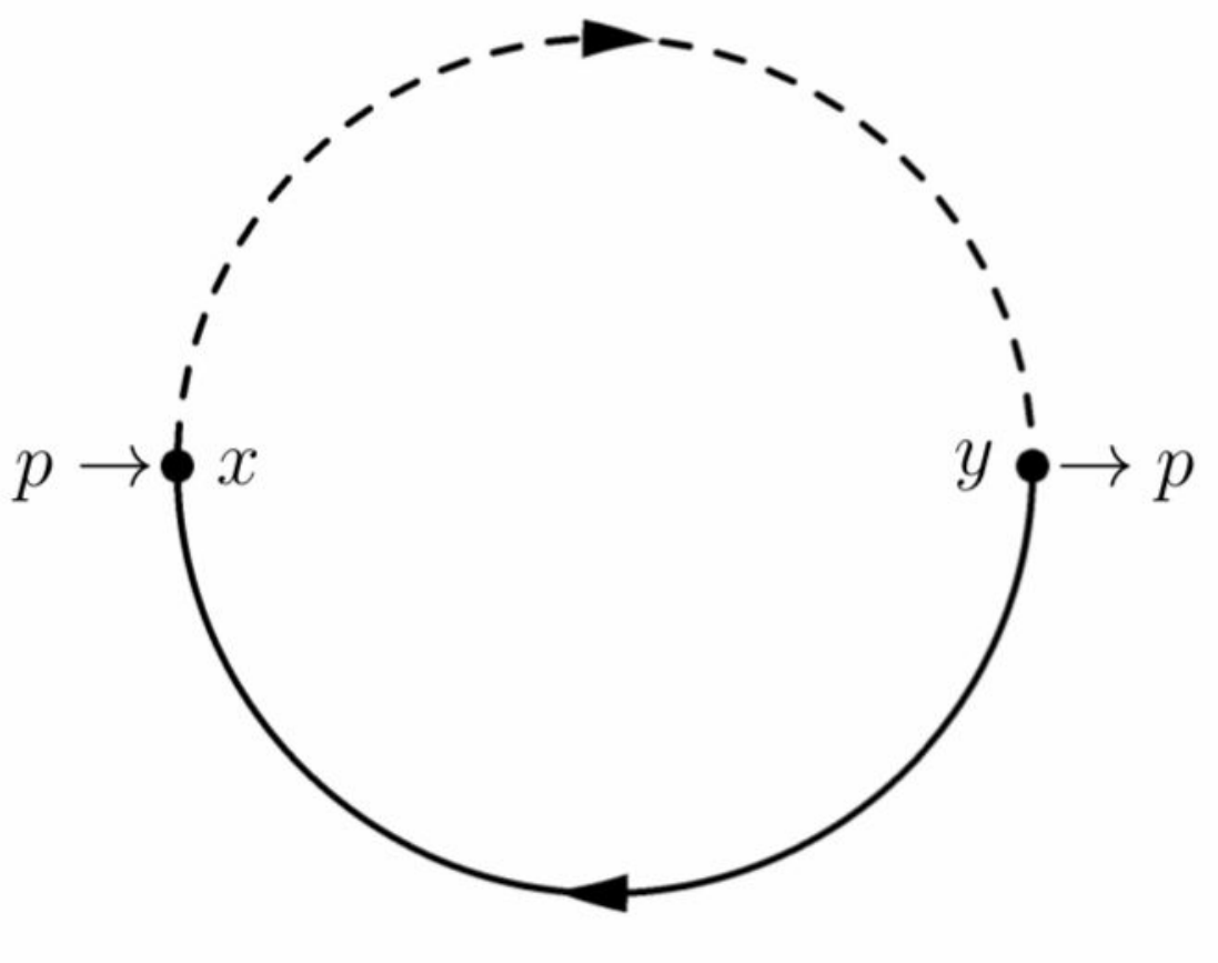
In this section, we integrate out (at one loop) a massive fermion that couples to a light scalar and a light fermion. Let us also focus specifically on the part of $\mathcal{L}_{\rm eff}$ containing two-fermion operators with additional covariant derivatives and field strengths but no scalar fields. In this case, the only relevant interaction at one-loop is

$$\mathcal{L}_{\rm int}=\bar{\Psi}C\Phi+h.c.\,,$$

(32)

where $\Psi$ is the fluctuation of the heavy fermion, $\Phi$ the one of the light scalar, and $C$ is a fermionic field-dependent coupling. As an example consider a heavy triplet fermion $\Psi^{a}$ coupled to the SM Higgs $\Phi^{i}$ and the top quark doublet $q_{L}^{j}$, in which case $C^{a}_{\ i}(x)=y(\sigma^{a})_{ij}q_{L}^{j}(x)$ where $y$ is a real coupling. Applying the Feynman rules to the diagram in fig. 1 gives

	$\displaystyle i\mathcal{L}_{\rm eff}$	$\displaystyle=$	$\displaystyle\int dt\,ds\,\biggl[\biggr.\int\frac{d^{d}k}{(2\pi)^{d}}\,e^{i(k^{2}-m^{2})t+i(k+i\partial_{x})^{2}s}$		(33)
			$\displaystyle\operatorname{tr}B^{s}(s;y,x)i\bar{C}(x)(\not{k}+m+i\not{D}_{x})B^{f}(t;x,y)iC(y)\biggl.\biggr]_{y=x}\,,$

where the trace is over the gauge indices, and we have defined the shorthands $B^{s}\equiv B(X=0)$, $B^{f}\equiv B(X_{f})$. Performing the Gaussian momentum integration yields

$$\begin{split}\mathcal{L}_{\rm eff}=&\frac{1}{(4\pi)^{\frac{d}{2}}}\int d\sigma d\tau\ \frac{e^{-m^{2}\tau}}{(\sigma+\tau)^{\frac{d}{2}}}\\ \biggl[\biggr.&-i\frac{\sigma}{\sigma+\tau}\,\exp\left(-\frac{\sigma\tau}{\sigma+\tau}\partial_{x}^{2}\right)\,\partial^{\mu}_{x}\operatorname{tr}B^{s}(-i\sigma;y,x)\bar{C}(x)\gamma_{\mu}B^{f}(-i\tau;x,y)C(y)\\ &+\exp\left(-\frac{\sigma\tau}{\sigma+\tau}\partial_{x}^{2}\right)\,\operatorname{tr}B^{s}(-i\sigma;y,x)\bar{C}(x)(m+i\not{D}_{x})B^{f}(-i\tau;x,y)C(y)\biggl.\biggr]_{y=x}\,,\end{split}$$

(34)

We have defined $\tau\equiv it$ and $\sigma\equiv is$, see discussion around eq. (31). Eq. (34) is the exact one-loop result to all orders in the operator dimension. To extract individual operators of a desired dimension, we expand the exponentials containing the partial derivative, as well as $B^{f}$ and $B^{s}$ according to eq. (6). In this particular example, the term proportional to $m$ will yield odd-dimensional operators (zero for chiral $C$), while the other terms will yield even dimensional ones. For a nontrivial example, consider the dimension-six operators:

$$\begin{split}\mathcal{L}&{}^{D=6}_{\rm eff}=(4\pi)^{-\frac{d}{2}}\int d\sigma d\tau\ \frac{e^{-m^{2}\tau}}{(\sigma+\tau)^{\frac{d}{2}}}\\ \biggl[\biggr.&-\frac{\sigma\tau}{\sigma+\tau}\,\partial^{\mu}_{x}\operatorname{tr}b_{0}^{s}(y,x)\bar{C}(x)\gamma_{\mu}b_{2}^{f}(x,y)C(y)-\frac{\sigma^{2}}{\sigma+\tau}\,\partial^{\mu}_{x}\operatorname{tr}b_{2}^{s}(y,x)\bar{C}(x)\gamma_{\mu}b_{0}^{f}(x,y)C(y)\\ &+i\frac{\sigma^{2}\tau}{(\sigma+\tau)^{2}}\,\partial_{x}^{2}\partial^{\mu}_{x}\operatorname{tr}b^{s}_{0}(y,x)\bar{C}(x)\gamma_{\mu}b_{0}^{f}(x,y)C(y)+\tau\,\operatorname{tr}b_{0}^{s}(y,x)\bar{C}(x)\gamma^{\mu}b^{f}_{2;\mu}(x,y)C(y)\\ &+\sigma\,\operatorname{tr}b_{2}^{s}(y,x)\bar{C}(x)\gamma^{\mu}b^{f}_{0;\mu}(x,y)C(y)-i\frac{\sigma\tau}{\sigma+\tau}\partial_{x}^{2}\operatorname{tr}b_{0}^{s}(y,x)\bar{C}(x)\gamma^{\mu}b_{0;\mu}^{f}(x,y)C(y)\biggl.\biggr]_{y=x}\,,\end{split}$$

(35)

where the semicolon denotes covariant differentiation, see eq. (58). Making use of the observation pointed out after eq. (19), many terms will be zero, the nonzero ones are:

$$\begin{split}\mathcal{L}&{}^{D=6}_{\rm eff}=\frac{1}{16\pi^{2}}\frac{1}{m^{2}}\biggl[\biggr.-\frac{1}{2}\operatorname{tr}\left(\bar{C}_{;\mu}\gamma^{\mu}{\left[b_{2}^{f}\right]}C+\bar{C}\gamma^{\mu}{\left[b_{2;\mu}^{f}\right]}C\right)+\left(\frac{3}{2}-\log\frac{m^{2}}{\mu^{2}}\right)\operatorname{tr}{\left[b_{2;;\mu}^{s\phantom{f}}\right]}\bar{C}\gamma^{\mu}C\\ &+\frac{i}{3}\operatorname{tr}\bar{C}_{;(\mu\nu\rho)}\gamma^{\mu}g^{\nu\rho}C+\operatorname{tr}\bar{C}\gamma^{\mu}{\left[b^{f}_{2;\mu}\right]}C-\frac{i}{2}g^{\nu\rho}\operatorname{tr}\left(2\bar{C}_{;\nu}\gamma^{\mu}{\left[b_{0;\mu\rho}^{f}\right]}C+\bar{C}\gamma^{\mu}{\left[b_{0;\mu\nu\rho}^{f}\right]}C\right)\biggl.\biggr]\,,\end{split}$$

(36)

where we already performed the integrals over $\tau$ and $\sigma$ given in App. C.2. The square brackets denote the LHKC’s, i.e. ${\left[b\right]}(x)\equiv b(x,x)$. Notice that at this point, all the ${\left[b\right]}^{\prime}s$ and $C^{\prime}s$ are evaluated at the same point $x$. Using the results from app. B, and making some simplifications, we arrive at

$$\mathcal{L}^{D=6}_{\rm eff}=\frac{1}{16\pi^{2}}\frac{1}{m^{2}}\biggl[\biggr.\frac{1}{8}\,\operatorname{tr}\bar{C}_{;\mu}\gamma^{\mu}(\not{F}^{f})C-\frac{1}{8}\operatorname{tr}C\not{F}^{f}\gamma^{\mu}C_{;\mu}+\frac{i}{3}\,\operatorname{tr}\bar{C}_{;(\mu\nu\rho)}\gamma^{\mu}g^{\nu\rho}C\\ +\left(\frac{1}{4}-\frac{1}{6}\log\frac{m^{2}}{\mu^{2}}\right)\,\operatorname{tr}F^{s}_{\mu\nu;\nu}\bar{C}\gamma^{\mu}C+\frac{1}{4}\operatorname{tr}\bar{C}\gamma^{\mu}F^{f}_{\mu\nu;\nu}C\biggl.\biggr]\,.$$

(37)

The calculation of these dimension-six operators in non-covariant perturbation theory would require the evaluation of 14 diagrams (not counting permutations of external legs), including some tedious Dirac algebra, plus the reconstruction of the covariant operators in terms of the noncovariant result.

In this section we would like to apply our formalism to integrate out a massive scalar coupled to gauge theory at two loops. As should be clear by now, our formalism contains roughly three main calculational steps: the Gaussian momentum integration, the reduction to local operators, and the integral over the Schwinger parameters. We will see that the first two steps are virtually identical at all loops, in particular, the momentum integration can be given in closed form, see eq. (83). The integrals over the Schwinger parameters become more involved at higher loops, in the example provided below they can however still be computed analytically.

Assuming that the heavy scalar does not acquire a vacuum expectation value, we can set the scalar background field to zero, that is, all the bilinear vertices in tab. 2 vanish in any gauge. The two-loop diagrams with at least one heavy propagator are the three sunset graphs and the figure-eight graph shown in fig. 2.

The figure-eight diagram gives

$$i\mathcal{L}^{\rm fig-8}_{\rm eff}=\frac{1}{2}\int dsdt\int\frac{d^{d}k}{(2\pi)^{d}}\frac{d^{d}k^{\prime}}{(2\pi)^{d}}\,e^{ik^{2}s+ik^{\prime 2}t-im^{2}s}\operatorname{tr}\left\{(ig^{2})\{\mathfrak{t}^{a},\mathfrak{t}_{b}\}B(s;x,x)\right\}B^{\mu b}_{\ \mu a}(t;x,x)$$

(38)

where the symmetry factor of $\frac{1}{2}$ results from the tadpole loop of the gauge boson. Performing the momentum integration yields

$$\mathcal{L}_{\rm eff}^{\rm fig-8}=\frac{g^{2}}{2(4\pi)^{d}}\int d\sigma\,e^{-m^{2}\sigma}\sigma^{-\frac{d}{2}}\operatorname{tr}\left\{\{\mathfrak{t}^{a},\mathfrak{t}_{b}\}B(-i\sigma;x,x)\right\}\int d\tau\,\tau^{-\frac{d}{2}}B^{\mu b}_{\ \mu a}(-i\tau;x,x)$$

(39)

Being a scaleless integral the $\tau$ integration gives zero in dimensional regularization.

Let us then evaluate the three sunset graphs. These diagrams also illustrate how derivative interactions are treated in our formalism. We mark a covariant derivative of a field by a star. The triple vertex connects to one scalar and one scalar with covariant derivative and hence each vertex carries one star, and the three diagrams represent the different ways of placing the stars in the diagram. The first two diagrams carry a symmetry factor of $\frac{1}{2}$ because the two vertices are equivalent, whereas the third diagram has no symmetry factor (the two vertices are not even the same, but rather complex conjugates).¹⁰¹⁰ 10 We further elaborate on symmetry factors in app. A.

Their contribution to the effective Lagrangian is

$$\begin{split}i\mathcal{L}_{\rm eff}=\int&drdsdt\biggl[\biggr.\int\frac{d^{d}k}{(2\pi)^{d}}\frac{d^{d}k^{\prime}}{(2\pi)^{d}}\,e^{ik^{2}r+ik^{\prime 2}s+i(k-k^{\prime}+i\partial_{x})^{2}t-im^{2}(s+r)}\\ \biggl(\biggr.\frac{1}{2}&\operatorname{tr}\left\{(g\mathfrak{t}^{a})(-ik_{\mu}+D^{x}_{\mu})B(r;x,y)(g\mathfrak{t}^{b})(-ik^{\prime}_{\nu}+D_{\nu}^{y})B(s;y,x)\right\}\\ +\frac{1}{2}&\operatorname{tr}\left\{(-g\mathfrak{t}^{a})(ik_{\nu}+D^{y}_{\nu})B(r;x,y)(-g\mathfrak{t}^{b})(ik^{\prime}_{\mu}+D_{\mu}^{x})B(s;y,x)\right\}\\ +&\operatorname{tr}\left\{(-g\mathfrak{t}^{a})B(r;x,y)(g\mathfrak{t}^{b})(-ik^{\prime}_{\nu}+D_{\nu}^{y})(ik^{\prime}_{\mu}+D^{x}_{\mu})B(s;y,x)\right\}\biggl.\biggr)B^{\mu\nu}_{ab}(t;x,y)\biggl.\biggr]_{y=x}\end{split}$$

(40)

The three traces correspond to the three diagrams. Notice how extra factors of $-ik_{\mu}+D_{\mu}$ etc. appear due to the propagators of derivatives of fields (denoted by stars in the diagrams), these derivatives are meant only to act on the $B$ factor immediately to the right (in contrast the partial derivative in the exponent which acts on all three $B$ factors). The Gaussian momentum integration is straightforward, see the master formula Eq. (83). Focusing for instance on the first diagram, one gets

$$\begin{split}\mathcal{L}^{(1)}_{\rm eff}=-&\frac{g^{2}}{2}\frac{1}{(4\pi)^{d}}\int d\varrho d\sigma d\tau\,\frac{e^{-m^{2}(\sigma+\varrho)}}{\omega^{\frac{d}{2}}}\\ \biggl[\biggr.&e^{-\frac{\varrho\sigma\tau}{\omega}\partial_{x}^{2}}\left(\frac{\tau}{2\omega}g_{\mu\nu}-\frac{\varrho\sigma\tau^{2}}{\omega^{2}}\partial_{\mu}^{x}\partial_{\nu}^{x}\right)\operatorname{tr}\left\{\mathfrak{t}^{a}B(-i\varrho;x,y)\mathfrak{t}^{b}B(-i\sigma;y,x)\right\}B^{\mu\nu}_{ab}(-i\tau;x,y)\\ +&e^{-\frac{\varrho\sigma\tau}{\omega}\partial_{x}^{2}}\left(\frac{\varrho\tau}{\omega}\partial^{x}_{\nu}\right)\operatorname{tr}\left\{\mathfrak{t}^{a}D^{x}_{\mu}B(-i\varrho;x,y)\mathfrak{t}^{b}B(-i\sigma;y,x)\right\}B^{\mu\nu}_{ab}(-i\tau;x,y)\\ +&e^{-\frac{\varrho\sigma\tau}{\omega}\partial_{x}^{2}}\left(-\frac{\sigma\tau}{\omega}\partial^{x}_{\mu}\right)\operatorname{tr}\left\{\mathfrak{t}^{a}B(-i\varrho;x,y)\mathfrak{t}^{b}D_{\nu}^{y}B(-i\sigma;y,x)\right\}B^{\mu\nu}_{ab}(-i\tau;x,y)\\ +&e^{-\frac{\varrho\sigma\tau}{\omega}\partial_{x}^{2}}\operatorname{tr}\left\{\mathfrak{t}^{a}D^{x}_{\mu}B(-i\varrho;x,y)\mathfrak{t}^{b}D_{\nu}^{y}B(-i\sigma;y,x)\right\}B^{\mu\nu}_{ab}(-i\tau;x,y)\biggl.\biggr]_{y=x}\end{split}$$

(41)

where $\omega\equiv\tau\sigma+\sigma\varrho+\varrho\tau$. Again this is the all-order result in the operator dimension. The other two diagrams are completely analogous. The next step would be to expand this result up to a desired order in the operator dimension, that is, perform the expansion of the exponentials containing the derivatives as well as the expansion eq. (6). There is nothing new to say here, this expansions work exactly as in the one-loop example. The resulting intergrals over the Schwinger parameters can still be performed analytically, see app. C.3.