Efficient Sensor Scheduling Strategy Based on Spatio-temporal Scope Information Model

Yang Liu Chen Dong* Xiaoqi Qin Xiaodong Xu Thanks: This work was supported in part by Beijing Natural Science Foundation under Grant No. 19L2033. (Corresponding author: Chen Dong.) Thanks: Yang Liu, Chen Dong, Xiaoqi Qin, and Xiaodong Xu are with the State Key Laboratory of Networking and Switching Technology, Beijing University of Posts and Telecommunications, Beijing, 100876, China. (e-mail: liu_young@bupt.edu.cn; dongchen@bupt.edu.cn; xiaoqiqin@bupt.edu.cn; xuxiaodong@bupt.edu.cn;).

Abstract

In this paper, based on the spatio-temporal correlation of sensor nodes in the Internet of Things (IoT), a Spatio-temporal Scope information model (SSIM) is proposed to quantify the scope valuable information of sensor data, which decays with space and time, to guide the system for efficient decision making in the sensed region. A simple sensor monitoring system containing three sensor nodes is considered, and two optimal scheduling decision mechanisms, single-step optimal and long-term optimal decision mechanisms, are proposed for the optimization problem. For the single-step mechanism, the scheduling results are analyzed theoretically, and approximate numerical bounds on the node layout between some of the scheduling results are obtained, consistent with the simulation results. For the long-term mechanism, the scheduling results with different node layouts are obtained using the Q-learning algorithm. The performance of the two mechanisms is verified by conducting experiments using the relative humidity dataset, and the differences in performance of the two mechanisms are discussed; in addition, the limitations of the model are summarized.

Index Terms:

Internet of Things, Spatio-temporal Scope Information Model, spatio-temporal correlation, sensor scheduling.

I Introduction

The Internet of Things connects the physical world and transforms physical objects from being traditional to smart by exploiting its underlying technologies such as ubiquitous and pervasive computing, embedded devices, communication technologies, sensor networks, Internet protocols and applications[1]. There are a large number of sensing nodes in the IoT, whose role is to collect data and provide information to the upper layers to make relevant adjustments and decisions for the whole system. Typical application scenarios include temperature and air quality monitoring in urban cities [2], smart traffic [3] and smart agriculture [4], etc. However, due to the cost constraints, most of the sensing nodes at the end of the network are usually low-cost sensors powered by batteries, which are very sensitive to power consumption, including micropower nodes and passive nodes. It has been one of the leading research problems to improve nodes sensing efficiency and prolong the nodes working life in these applications.

For some time-sensitive applications, the requirement for data immediacy is stronger, i.e., outdated data is not of much value to the system. Based on this idea, the concept of Age of Information (AoI) [5] is proposed, which is defined as the time difference between the moment of sensing data generation and the moment of acceptance by the receiver. On the one hand, the system expects nodes to send frequent updates so as to be able to ensure the immediacy of data information, but on the other hand, frequent updates can cause congestion in the system and consume too much energy of nodes, resulting in poor performance. Therefore, numerous scholars have studied the trade-off strategy of the system by combining AoI with various queuing and communication models. Specifically, the optimal service rates to minimize the average AoI in different queuing models are derived in [5]. The problem of minimizing the expected weighted sum AoI while simultaneously satisfying timely-throughput constraints is addressed in [6]. Reference [7] investigates the problem of minimizing average and peak age of information (PAoI) under general interference constraints. A discrete-time queueing model to derive the exact distributions of the AoI and PAoI sequences in a multisource status update system is proposed in [8]. In [9], it is found that the optimal arrival-independent renewal (AIR) scheduling policy to minimize the time-average AoI is RR-ONE, i.e., scheduling terminals in a round-robin fashion, and each terminal only retains the most up-to-date packet. Reference [10] studies the optimal device scheduling process that jointly minimizes the average AoI and the energy cost with two types of correlated devices.

The freshness of information is linearly decreasing in the definition of AoI, but there is some correlation in the time domain due to the physical nature of monitoring sources, which may cause the performance degradation due to information aging is not a linear function of time. Therefore, some scholars have proposed nonlinear functions about AoI and conducted related researches Reference [11] introduces a general age penalty function to characterize the level of dissatisfaction on data staleness. In [12], a general expression of the generating function of AoI and the peak age of information (PAoI) metric is provided, which provides a methodology for analyzing general non-linear age functions. Exploiting the temporal correlation between consecutive samples of a Markov source, reference [13] considers a generalized incremental update scheme by sending differential updates.

In addition, the dense deployment of sensing nodes on the space inevitably causes the observations of the nodes to be highly correlated in the spatial domain. Therefore, some scholars have studied the layout setting of nodes on the spatial domain and the spatial critical sampling rate, etc. The correlation between nodes is used to reconstruct the observed physical phenomena based on a fraction of all available sensor nodes in [14], where a framework for the analysis of sensor density based on asymptotic analysis is proposed. In [15], a theoretical analysis of spatio-temporal correlation characteristics of point and field sources in WSN is performed, and the spatio-temporal characteristics are analytically derived along with the distortion functions. Based on the confident information coverage (CIC) model, [16] and [17] study the critical sensor density and find the optimal placement pattern to achieve complete coverage in randomly deployed sensor networks. In addition, a node deployment scheme to maximize the network lifetime and ensure CIC in a field with obstacles is proposed in [18].

Meanwhile, some scholars have simultaneously investigated the cooperative scheduling and spatio-temporal sampling rate among nodes in conjunction with the correlation of nodes in time and space domain. In [19], a theoretical framework to capture the spatial and temporal correlations in wireless sensor networks is first introduced, which constitutes a basis for the development of such energy-efficient communication protocols for Wireless Sensor Networks (WSN). More work related to this paper in this regard is described in detail in subsection B.

The main idea of this paper is to measure the value of real-time useful information of sensor data in the temporal and spatial domains by using the spatio-temporal correlation of the sources. For example, the first data of sensors collected continuously in the time domain can bring the most amount of valuable information due to the lack of a priori knowledge, while the later data in the time domain can bring less valuable information than the first data due to the short time correlation of the physical properties of the sources, i.e., the first data can provide a certain amount of priori information for the later ones. Similarly, there is an overlap in the valuable information provided by the data acquired simultaneously by nodes close to each other in the spatial domain. In this paper, a model to measure real-time valuable information of sensor data is established to represent the effective spatio-temporal scope of data information, and the optimal node scheduling strategy under different node layouts is investigated to improve the efficiency of sensing information.

I-A Contributions and Paper Outline

In this paper, utilizing the spatio-temporal correlation of the sources in the area to be measured, we establish a Spatio-temporal Scope Information Model, which measure the effective information spatio-temporal domian of node data for the whole system in real time. In simple terms, the information value of a sensor data gradually decays in the temporal domain with the passage of time, and it also gradually decays in the neighborhood of the node location in the spatial domain. Moreover, this paper investigates the efficient activation scheduling scheme for three nodes in different location layouts to ensure the effective grasp of the system over the whole area. The main contributions of this paper are as follows.

1.

Utilizing the spatio-temporal correlation of sensor nodes, a Spatio-temporal Scope Information Model is proposed to quantify the valuable information of sensor data, which decays with space and time.
2.

A single-step optimal decision-making mechanism for a three-node sensing system is proposed. The theoretical analysis is made, and a method to solve the boundary node distribution among various scheduling situations is provided.
3.

A long-term optimal decision-making mechanism for a three-node sensing system is proposed, which is modeled as a Markov decision process, and the Q-learning algorithm is utilized to solve the optimal scheduling results.
4.

With single-step mechanism, the approximate bounds for the node layout between partial scheduling results are obtained from theoretical analysis and numerical calculation, which match with the simulation results. The optimal scheduling results with long-term mechanism corresponding to different node layout are obtained. Finally, the different performances of the two mechanisms are experimentally verified, and the advantages and limitations of each are summarized.

The rest of the paper is organized as follows: In Section II, the system model and optimization problem are described. In Section III, a optimal decision-making mechanism of single-step information acquisition is proposed for the established model, and the related theoretical analysis is made. In Section IV, a optimal decision-making mechanism of long-term information acquisition is proposed and the modeling and solution methods are described. In Section V, numerical results and simulation results are presented. In Section VI, experimental evaluation is performed. Finally, conclusions are drawn and discussions are made in Section VII.

I-B Related work

TABLE I: Comparison of References.

[b] Reference information source sensors correlation metrics Research results [20] Single-point Two Spatial-temporal Estimation Error optimal time shift between two sensors [21], [22] multi-point Multiple Spatial-temporal Estimation Error DRL -based scheduling mechanism [24], [25] Single-point (noisy Ornstein- Uhlenbeck process) Single source and noise mutual information closed-form VoI expressions [26], [27] Regional Multiple Spatial-temporal error-tolerable sensing (ETS) coverage AoI violation probability, optimal sensors transmission power [28] Regional Multiple Spatial-temporal Node Spatial-temporal coverage radius Node activation scheduling [29], [30] time-varying Gauss- Markov Random Field (GMRF) Multiple Spatial-temporal mean squared estimation error Closed-form expressions for estimation error, optimal Spatial-temporal sampling rates [31], [32] N Gaussian process Multiple Spatial-temporal mean squared error (MSE) optimal scheduling policy [33] Single-point Multiple Spatial-temporal Spatial-temporal mutual information optimal update interval [34] multi-point Multiple Spatial-temporal overall utility of information update Status update node set this work Regional Three Spatial-temporal Spatial-temporal Scope information Node activation strategy in any layout

Among some recent studies, the following ones are more relevant to the work of this paper. Specifically, reference [20] considers a system consisting of two correlated information sources ,and establishes a minimal time shift between the two sources’ updates, for which the system estimation error is minimal. An energy-aware scheduling mechanism based on Deep Reinforcement Learning (DRL) is proposed in [21] and [22], which is capable of significantly prolonging the lifetime of a network of battery-powered sensors. A measure for the freshness of information is proposed in [23], which uses the mutual information between the real-time source value and the delivered samples at the receiver. In [24] and [25], a mutual-information based Value of Information (VoI) framework is formalised to characterise how valuable the status updates are for Hidden Markov Models. An error-tolerable sensing (ETS) coverage as the area where the estimated information is with smaller error than the target value is defined in [26] and [27], where the $\eta$ -coverage probability is presented, and the optimal transmission power which minimizes the average energy consumption while guaranteeing a certain level of the $\eta$ -coverage probability is provided. In [28], a transmission scheduling approach is presented through a geometric approach with individual node coverage model, which is a function of the estimation accuracy in a region near the node. The performance of state updates is studied in [29] and [30], where the status is modeled as a time-varying Gauss-Markov Random Field (GMRF) and the estimation error of status update at the fusion center is analyzed. In [31] and [32], an optimal scheduling policy for transmitting observations of spatio-temporally dependent processes over a limited number of communication channels is derived that minimizes the time-average mean squared error (MSE), resulting in a periodic scheduling sequence. A novel timeliness metric spatially temporally correlative mutual information (STI) is proposed in [33], where an optimal update interval is found by solving an integer optimization problem about slot allocation in satellite. Assuming that each information can be commonly observed by multiple sensors, two multi-source information update problems, named AoI-aware Multi-Source Information Updating (AoI-MSIU) and AoI-Reduction-aware Multi-Source Information Updating (AoIR-MSIU) problems, are formulated in [34].

Table I shows in detail the comparison between our work and the above references. Throughout the above studies, although many scholars have studied the cooperative scheduling and sampling strategies among nodes by combining the spatio-temporal correlation of the sources, less attention has been devoted to all possible scheduling results and change rules of the scheduling results for different node layouts with an effective grasp of the whole region. For detail, this paper discusses the node sequential activation scheduling problem for different node layout cases. It is the main motivation of this paper to study the possible optimal scheduling results for different node layout cases, and analyze the change law of optimal scheduling results for different node layouts.

II System model and Problem formulation

II-A System model

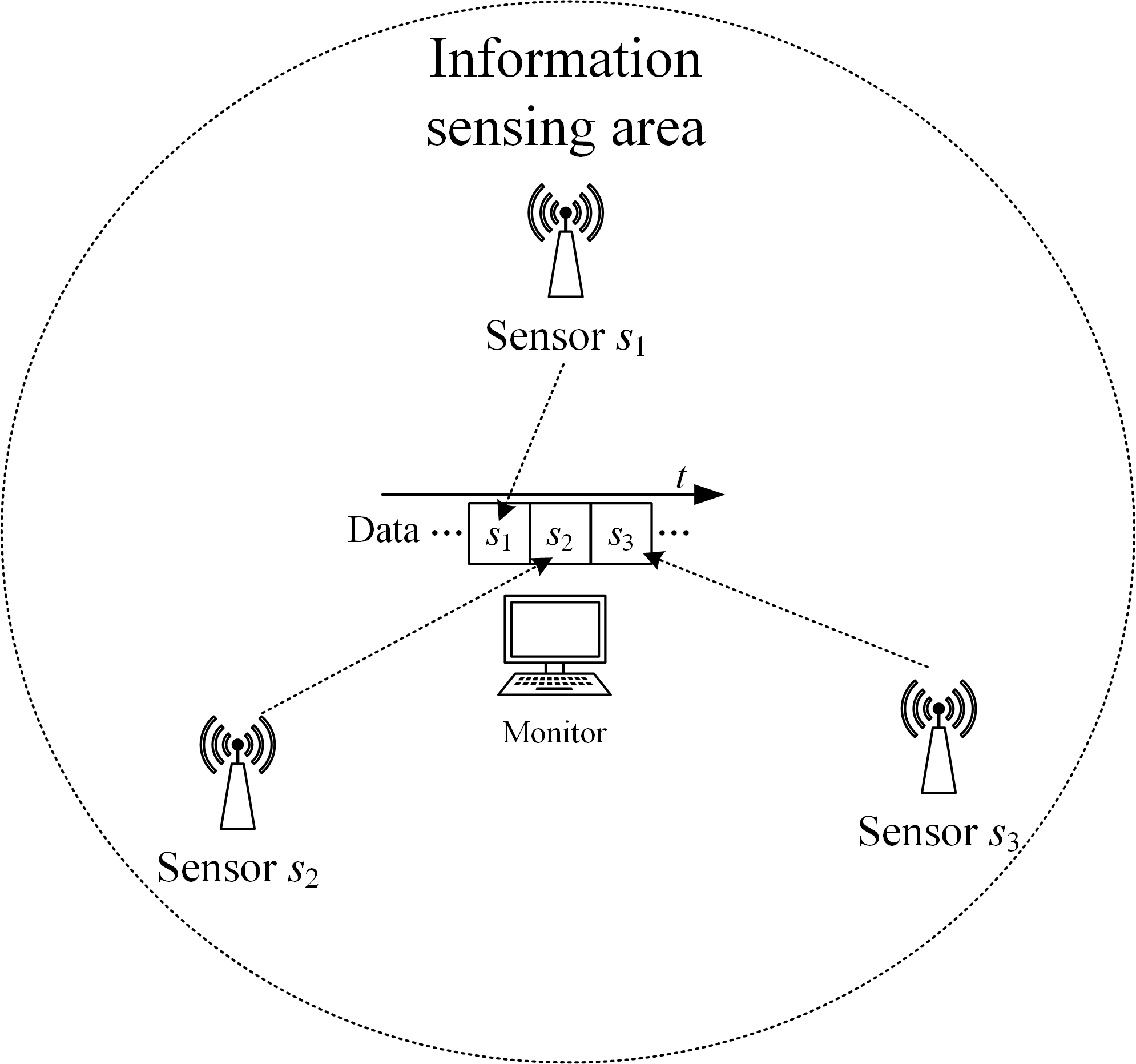
In this paper, we mainly consider a simple sensing system composed of three sensing nodes, where the information sensing area is the whole two-dimensional (2D) plane, and the importance attached to each location in the area is the same, that is, there is no setting of sensing priority, as shown in Fig. 1. For the convenience of preliminary analysis, it is assumed that the system periodically decides to activate a sensing node for information acquisition, i.e., the interval time between each decision is constant. The data transmission conditions are assumed to be ideal, ignoring the influence of data sending and transmission, i.e., it is assumed that the monitor can receive sensor data immediately after the node is activated.

II-B Spatio-temporal Scope Information Model

In this paper, a Gaussian random field is assumed in the two-dimensional region to be measured, i.e., the variables to be measured between any points in space conform to the joint Gaussian distribution. Without considering the node hardware acquisition error, i.e., the data collected by the nodes are considered accurate enough to completely represent the values of the random variables to be measured. Then, for a certain node, let the random variable to be monitored corresponding to the spatial location of the node be $X$ . The amount of valuable information that the first activation of the node can bring to $X$ is the entropy $H(x)$ . Meanwhile, for any point $p$ in the neighborhood near the node, let its corresponding random variable be $Y_{p}$ , and $Y_{p}$ and $X$ conform to the joint Gaussian distribution. Denote the correlation coefficient as $\rho$ , then the amount of information that the node data can provide at position $p$ is

I(p)=I(Y_{p};X)=h(Y_{p})-h(Y_{p}|X)=-\frac{1}{2}\log(1-{{\rho}^{2}})

(1)

Then the total amount of information in the two-dimensional plane is

\begin{split}{{I}_{D}}&=\int_{0}^{2\pi}{\int_{0}^{1}{-\frac{1}{2}\log(1-{{\rho}^{2}})\cdot\rho\cdot d\theta d}}\rho\\ &=-\frac{\pi}{2}\int_{0}^{1}{\log(1-{\rho}^{2})d{{\rho}^{2}}}=\frac{\pi}{2}\end{split}

(2)

It can be seen from the above equation that although the information calculation result in Eq. (1) tends to infinity when the correlation coefficient $\rho$ tends to $1$ , the total scope information integral in the two-dimensional plane converges and can be calculated. In this paper, for simplicity, we consider the spatiotemporally separable covariance function [20]

\rho={{e}^{-{{\lambda}_{d}}\cdot d-{{\lambda}_{t}}\cdot t}}

(3)

where $d$ represents the spatial distance, and $t$ represents the time difference, in addition, $\lambda_{d}$ and $\lambda_{t}$ are the scaling parameters of information relevance with respect to space and time, respectively. The above description is for a single node and the first activation of the information acquisition. However, when the system has multiple nodes and the nodes are activated in a certain order, there will be multiple nodes with spatio-temporal association at each location in the two-dimensional plane. In other words, at any point in space, the previous sensor data of each node can provide a certain amount of information and eliminate part of the uncertainty. In this paper, for the sake of simplicity, the system keeps only the latest sensor data of each node, and only the sensor data that can eliminate the most uncertainty and provide the most information at that location is selected to provide a reference for that location. In other words, it is considered that the node data closest to the location in terms of spatio-temporal domian, i.e., the most relevant node data, provides information for that location, and the amount of joint information provided by multiple nodes previous data together is not considered. That is, the amount of information available for the system at any point $p$ in the two-dimensional plane at moment $t$ is

I(p,t)=-\frac{1}{2}{{\log}}\left(1-{{e}^{-2{{\lambda}_{d}}\cdot|p-{{p}^{*}}(p)|-2{{\lambda}_{t}}\cdot|t-{{t}^{*}}(p)|}}\right).

(4)

where ${p^{*}}(p)$ is the node location coordinates of the most relevant sensor data in space-time for location $p$ , and

{{p}^{*}}(p)=\mathop{\arg\min}\limits_{p_{s_{i}}}{{\lambda}_{d}}|p-p_{s_{i}}|+{{\lambda}_{t}}|t-t_{s_{i}}|,\ p_{s_{i}}\in S,

(5)

where $S$ is the set of all node coordinates. Furthermore, $|t-{{t}^{*}}(p)|$ in Eq. (4) is the value of AoI for the most relevant data at position $p$ at the current moment. According to the above equation, the spatio-temporal scope information map of the system at time t for the whole 2D space can be obtained as illustrated in Fig. 2, where the vertical height represents the amount of valuable information, and the location of the peak is the sensing nodes location.

At this moment, if the node $s_{i}$ is activated, the incremental information that can be obtained for each point $p$ in the 2D plane is

\begin{split}&inf{{o}_{gain}}(p,s_{i})=h({{Y}_{p}}|{{X}_{past}^{*}})-h({{Y}_{p}}|{{X}_{{{s}_{i}}}})\\ &=\left[h({{Y}_{p}})-h({{Y}_{p}}|{{X}_{{{s}_{i}}}})\right]-\left[h({{Y}_{p}})-h({{Y}_{p}}|{{X}_{past}^{*}})\right]\\ &=-\frac{1}{2}\log\frac{1-{{e}^{-2{{\lambda}_{d}}\cdot|p-{{p}_{{{s}_{i}}}}\text{ }\!\!|\!\!\text{ }}}}{1-{{e}^{-2{{\lambda}_{d}}\cdot|p-{{p}^{*}}(p)|-2{{\lambda}_{t}}\cdot AoI^{*}(p)}}}\end{split}

(6)

where ${Y}_{p}$ is the random variable corresponding to position p, $X_{s_{i}}$ is the random variable corresponding to position of node $s_{i}$ , and ${X}_{past}^{*}$ is the random variable corresponding to the most relevant node data at position $p$ . In addition, $AoI^{*}(p)$ is the AoI value of the most spatiotemporally relevant data at position $p$ . However, each time a sensor node activated by system may acquire no new valuable information in certain regions. In other words, the previous data of other nodes provide more information in these regions than the node activated at this moment, and the result of the above equation takes a negative value in these regions, but which does not meet the definition of information. Because no more information can be provided, but temporarily no loss is caused. Thus, the information increment that can be obtained in these areas is defined as 0, i.e., the scope information increment in the whole two-dimensional plane of the activated node $s_{i}$ is

\begin{split}&{{I}_{gain}}=\iint\limits_{D}{\max\{inf{{o}_{gain}}(p,s_{i}),0\}}d\sigma\\ &=\iint\limits_{D}{\max\left\{-\frac{1}{2}\log\frac{1-{{e}^{-2{{\lambda}_{d}}\cdot|p-{{p}_{{{s}_{i}}}}\text{ }\!\!|\!\!\text{ }}}}{1-{{e}^{-2{{\lambda}_{d}}\cdot|p-{{p}^{*}}(p)|-2{{\lambda}_{t}}\cdot AoI^{*}(p)}}},0\right\}}d\sigma\\ \end{split}

(7)

II-C Problem formulation

In this paper, it is the research objective to find the most efficient way of node activation scheduling given the node location layout and the spatio-temporal correlation coefficient of the region to be measured. That is, it is desired that the total amount of information mastered by the system for the entire two-dimensional plane has the maximum mean value in time domian, as in the following equation

\max\overline{I}=\underset{T\to\infty}{\mathop{\lim}}\,\frac{1}{T}\int_{0}^{T}{\big[\iint\limits_{D}{I(p,t)d\sigma}\big]}dt

(8)

Let the total amount of information held by the system at each activation node moment $t_{i}$ be $I_{i}$ , that is,

{{I}_{i}}=\iint\limits_{D}{I(p,{{t}_{i}})d\sigma}.

(9)

and let the total two-dimensional information decay function after the $i_{th}$ activation node of the system be $f_{i}(t)$ as follows

{{f}_{i}}(t)=\frac{\iint\limits_{D}{-\frac{1}{2}{{\log}_{2}}\left(1-{{e}^{-2{{\lambda}_{d}}\cdot|p-{{p}^{*}}(p)|-2{{\lambda}_{t}}\cdot[Ao{{I}^{*}}(p)+t]}}\right)}d\sigma}{\iint\limits_{D}{-\frac{1}{2}{{\log}_{2}}\left(1-{{e}^{-2{{\lambda}_{d}}\cdot|p-{{p}^{*}}(p)|-2{{\lambda}_{t}}\cdot Ao{{I}^{*}}(p)}}\right)}d\sigma}

(10)

Letting $T=n*\Delta t$ , the expression for the information mean can be further written as

\begin{split}\bar{I}=\underset{n\to\infty}{\mathop{\lim}}\,\frac{\sum\limits_{i=1}^{n}{{{I}_{i}}\cdot\int_{0}^{\Delta t}{{{f}_{i}}(t)dt}}}{n\cdot\Delta t}\end{split}

(11)

and the following relationship holds for the total amount of two-dimensional information and the incremental information of the activated nodes

{{I}_{i+1}}={{I}_{i}}\cdot{{f}_{i}}(\Delta t)+{{I}_{gain}}(i),\ i=1,2,3,\cdots

(12)

Recursive induction of the above equation leads to the following result

\begin{split}{{I}_{n}}&={{I}_{gain}}(n)+\sum\limits_{i=1}^{n-1}{\left[{{I}_{gain}}(i)\cdot\prod\limits_{j=i}^{n-1}{{{f}_{j}}(\Delta t)}\right]},\\ \end{split}

(13)

then,

\begin{split}&\sum\limits_{i=1}^{n}{{{I}_{i}}\cdot\int_{0}^{\Delta t}{{{f}_{i}}(t)dt}}\\ =&\sum\limits_{i=1}^{n}{\left[\left({I}_{gain}(i)+\sum\limits_{j=1}^{i-1}{{{I}_{gain}}(j)\cdot\prod\limits_{k=j}^{i-1}{{{f}_{k}}(\Delta t)}}\right)\cdot\int_{0}^{\Delta t}{{{f}_{i}}(t)dt}\right]}\\ =&\sum\limits_{i=1}^{n}\left\{{{{I}_{gain}}(i)\cdot}\left[\sum\limits_{j=i}^{n}{\left(\int_{0}^{\Delta t}{{{f}_{j}}(t)dt}\cdot\prod\limits_{k=i}^{j-1}{{{f}_{k}}(\Delta t)}\right)}\right]\right\}.\\ \end{split}

(14)

The above equation is difficult to continue to derive, mainly because $f_{i}(t)$ is challenging to get a clear closed form, so here it is proposed to unify the total information decay of all moments approximately expressed as $f(t)$ , that is,

{{f}_{i}}(t)\approx f(t),i=1,2,3\cdots.

(15)

In other words, it is assumed that the total information decay trend is uniform at all activation node moments. The reason for such an approximate assumption here is mainly motivated by the consideration that the system tends to acquire more and smoother information, which leads to similar total information at each activation node moment, thus causing the decay trend may be approximately the same. Then Eq. (14) can be further written as

\begin{split}&\int_{0}^{\Delta t}{f(t)dt}\cdot\sum\limits_{i=1}^{n}{\left({{I}_{gain}}(i)\cdot\sum\limits_{j=0}^{n-i}{f{{(\Delta t)}^{j}}}\right)}\\ =&\int_{0}^{\Delta t}{f(t)dt}\cdot\sum\limits_{i=1}^{n}{\left({{I}_{gain}}(i)\cdot\frac{1-f{{(\Delta t)}^{n-i+1}}}{1-f(\Delta t)}\right)}\\ =&\frac{\int_{0}^{\Delta t}{f(t)dt}}{1-f(\Delta t)}\cdot\sum\limits_{i=1}^{n}{\left[{{I}_{gain}}(i)\cdot\left(1-f{{(\Delta t)}^{n-i+1}}\right)\right]}\end{split}

(16)

Since $f(\Delta t)$ ¡ 1, for any positive number $\varepsilon$ that is greater than 0 and small enough,

\begin{split}&1-f{{(\Delta t)}^{n-i+1}}<1-\varepsilon\\ &i>n+1-{{\log}_{f(\Delta t)}}\varepsilon,\\ \end{split}

(17)

so when $n$ tends to infinity, the percentage of terms with information increment $I_{gain}(i)$ coefficients less than $1-\varepsilon$ is

\underset{n\to\infty}{\mathop{\lim}}\,\frac{{{\log}_{f(\Delta t)}}\varepsilon}{n}=0.

(18)

Therefore the coefficients can be approximated by 1, i.e., the optimization problem becomes the following form

\begin{split}\max\ &\bar{I}=\frac{\int_{0}^{\Delta t}{f(t)dt}}{\Delta t\left(1-f(\Delta t)\right)}\cdot\underset{n\to\infty}{\mathop{\lim}}\,\cdot\frac{1}{n}\sum\limits_{i=1}^{n}{{{I}_{gain}}(i)}\\ \text{s}\text{.t}\text{. }&Se({{t}_{i}})={{s}_{i}}\in\left\{{{s}_{1}},{{s}_{2}},{{s}_{3}}\right\}\\ &{{t}_{i}}=0,\Delta t,2\Delta t,\cdots,n\Delta t,\\ \end{split}

(19)

where $Se(t_{i})$ is the node activated at the moment $t_{i}$ . From the above expression, the original problem is converted to the problem of maximizing the mean value of the incremental information obtained by each activated node.

III Single-step optimal mechanism

Regarding the above-mentioned problems, the first optimization mechanism readily comes to mind is the single-step decision method, which means that the system computationally finds out the sensing node that can obtain the most information increment at the current moment based on the known spatio-temporal information residual map, then makes it active and updates the spatio-temporal information map. The system takes the same actions at each discrete decision moment after that. The mathematical expression as a rule for each node activation $s_{i}$ can be written as follows

Se(t_{i})={\underset{s_{i}\in\left\{{{s}_{1}},{{s}_{2}},{{s}_{3}}\right\}}{\arg\max}\,\iint\limits_{D}{\max\{inf{{o}_{gain}}(p,s_{i}),0\}}d\sigma}.

(20)

where ${{p}_{{{s}_{i}}}}$ is the position coordinate of the activated sensing node. According to whether the value of the latter term in the integral equation is greater than 0, the integration region can be divided into two parts, $D^{\prime}$ and $D^{\prime\prime}$ , thus the integral in Eq. (20) is equivalent to

\iint\limits_{D^{\prime}}{-\frac{1}{2}\log\frac{1-{{e}^{-2{{\lambda}_{d}}\cdot|p-{{p}_{{{s}_{i}}}}\text{ }\!\!|\!\!\text{ }}}}{1-{{e}^{-2{{\lambda}_{d}}\cdot|p-{{p}^{*}}(p)|-2{{\lambda}_{t}}\cdot AoI^{*}(p)}}}}d\sigma,

(21)

where $D^{\prime}$ and $D^{\prime\prime}$ are the set consisting of points that respectively satisfy the following conditions:

\left\{\begin{split}&p\in D^{\prime},\ |p-{{p}_{{{s}_{i}}}}|-|p-{{p}^{*}}(p)|<\frac{{{\lambda}_{t}}}{{{\lambda}_{d}}}\cdot|t-{{t}^{*}}(p)|\\ &p\in D^{\prime\prime},\ |p-{{p}_{{{s}_{i}}}}|-|p-{{p}^{*}}(p)|\geq\frac{{{\lambda}_{t}}}{{{\lambda}_{d}}}\cdot|t-{{t}^{*}}(p)|.\end{split}\right.

(22)

In addition, the most spatially and temporally correlated node $p^{*}(p)$ varies for different locations $p$ with the following equations:

\begin{split}{{p}^{\text{*}}}(p)\text{=}&\arg\min{{\lambda}_{d}}|p-{{p}^{*}}(p)|+{{\lambda}_{t}}|t-{{t}^{*}}(p)|\\ =&\begin{cases}{{p}_{{{s}_{1}}}},&p\in{{S}_{1}}\\ {{p}_{{{s}_{2}}}},&p\in{{S}_{2}}\\ {{p}_{{{s}_{3}}}},&p\in{{S}_{3}},\\ \end{cases}\end{split}

(23)

where $S_{1}$ , $S_{2}$ and $S_{3}$ are the sets of points that respectively meet the conditions as Eq. (24),

\left\{\begin{split}{{S}_{1}}=\left\{p\in D\Big||p-{{p}_{{{s}_{1}}}}|-|p-{{p}_{{{s}_{2}}}}|<\frac{{{\lambda}_{t}}}{{{\lambda}_{d}}}\cdot({{AoI}_{{{s}_{2}}}}-{{AoI}_{{{s}_{1}}}}),\ |p-{{p}_{{{s}_{1}}}}|-|p-{{p}_{{{s}_{3}}}}|<\frac{{{\lambda}_{t}}}{{{\lambda}_{d}}}\cdot({{AoI}_{{{s}_{3}}}}-{{AoI}_{{{s}_{1}}}})\right\}&\\ {{S}_{2}}=\left\{p\in D\Big||p-{{p}_{{{s}_{2}}}}|-|p-{{p}_{{{s}_{1}}}}|<\frac{{{\lambda}_{t}}}{{{\lambda}_{d}}}\cdot({{AoI}_{{{s}_{1}}}}-{{AoI}_{{{s}_{2}}}}),\ |p-{{p}_{{{s}_{2}}}}|-|p-{{p}_{{{s}_{3}}}}|<\frac{{{\lambda}_{t}}}{{{\lambda}_{d}}}\cdot({{AoI}_{{{s}_{3}}}}-{{AoI}_{{{s}_{2}}}})\right\}&\\ {{S}_{3}}=\left\{p\in D\Big||p-{{p}_{{{s}_{3}}}}|-|p-{{p}_{{{s}_{1}}}}|<\frac{{{\lambda}_{t}}}{{{\lambda}_{d}}}\cdot({{AoI}_{{{s}_{1}}}}-{{AoI}_{{{s}_{3}}}}),\ |p-{{p}_{{{s}_{3}}}}|-|p-{{p}_{{{s}_{2}}}}|<\frac{{{\lambda}_{t}}}{{{\lambda}_{d}}}\cdot({{AoI}_{{{s}_{2}}}}-{{AoI}_{{{s}_{3}}}})\right\}&.\end{split}\right.

(24)

in which the ${{AoI}_{{{s}_{1}}}}$ , ${{AoI}_{{{s}_{2}}}}$ and ${{AoI}_{{{s}_{3}}}}$ are the AoI of the latest sensing data of each node. The increment of information that can be obtained by the activated node $s_{i}$ from the above expression can be written as

\begin{split}I_{gain}=&\sum\limits_{j=1}^{3}{\iint\limits_{{{S}_{j}}}{\max\{inf{{o}_{gain}}(p,s_{i}),0\}}d\sigma}\\ =&\sum\limits_{j=1}^{3}{\iint\limits_{{{S}_{j}}^{\prime}}{{info_{gain}}(p,s_{i})}d\sigma},\end{split}

(25)

where $S_{j}^{\prime}$ is the set of points that meet the condition as

|p-{{p}_{{{s}_{i}}}}|-|p-{{p}_{{{s}_{j}}}}|<\frac{{{\lambda}_{t}}}{{{\lambda}_{d}}}\cdot{AoI}_{{{s}_{j}}},\ p\in{{S}_{j}},\ j\in\left\{1,2,3\right\}.

(26)

From the fact that the trajectory of a point in plane geometry where the difference between the distances to two points is fixed is a hyperbola, we can preliminarily determine that the boundary of the above set $D^{\prime}$ may contain several curves. For example, when the system only has two nodes, and ${{p}_{{{s}_{i}}}}$ , ${{p}^{*}}(p)$ are taken as ${{p}_{{{s}_{1}}}}$ , ${{p}_{{{s}_{2}}}}$ , respectively, let the coordinates of node $s_{1}$ and node $s_{2}$ in 2D space be $(-c,0)$ , $(c,0)$ as shown in Fig. 3(a). From the property that the difference between two sides of a triangle is less than the third side, it is easy to obtain the inequality as follows:

|p-{{p}_{{{s}_{1}}}}|-|p-{{p}_{{{s}_{2}}}}|<d_{s_{1},s_{2}}=2c.

(27)

Abbreviating $\frac{{{\lambda}_{t}}}{{{\lambda}_{d}}}\cdot\Delta t$ to $2a$ , the inequality corresponding to the set $D^{\prime\prime}$ can be written as

\begin{matrix}&2c>|p-{{p}_{{{s}_{1}}}}|-|p-{{p}_{{{s}_{2}}}}|\geq\frac{{{\lambda}_{t}}}{{{\lambda}_{d}}}\cdot\Delta t=2a>0\\ \Leftrightarrow&\frac{{x}^{2}}{{a}^{2}}-\frac{{{y}^{2}}}{{{c}^{2}}-{{a}^{2}}}\geq 1,\ x>0,\ c>a>0,\end{matrix}

(28)

and $D^{\prime\prime}$ is an empty set when $c<a$ , i.e., $d_{s_{1},s_{2}}<\frac{{{\lambda}_{t}}}{{{\lambda}_{d}}}\cdot\Delta t$ , in which case, a certain increment of information can be obtained in the whole 2D plane. However, it should be noted that activating node $s_{1}$ or node $s_{2}$ can obtain the same incremental information at this point, and there is no optimal activation scheme from the perspective of information acquisition only. Therefore, in the subsequent analytical modelling, the distance between the nodes must be at least greater than $\frac{{{\lambda}_{t}}}{{{\lambda}_{d}}}\cdot\Delta t$ .

The area distribution of $D^{\prime\prime}$ that can be obtained from Eq. (28) is shown in the shaded part of Fig. 3(a), and no new information increment can be obtained by activating node $s_{1}$ in this area. The remaining blank areas are where new information increments can be obtained, that is, the set $D^{\prime}$ . The boundary curve formula of the $D^{\prime\prime}$ is required for the expression of the information increment’s integral limit to calculate the information increment’s value.

However, due to different node positions and different angles of the coordinate system, when the horizontal axis of the curve is not parallel to the x-axis, a 2D rotation matrix can be used to derive the equation of the curve $\frac{{{x}^{2}}}{{{a}^{2}}}-\frac{{{y}^{2}}}{{{b}^{2}}}=1$ after rotating $\theta$ counterclockwise around the origin as

(\frac{{{\cos}^{2}}\theta}{{{a}^{2}}}-\frac{{{\sin}^{2}}\theta}{{{b}^{2}}}){{x}^{2}}+(\frac{{{\sin}^{2}}\theta}{{{a}^{2}}}-\frac{{{\cos}^{2}}\theta}{{{b}^{2}}}){{y}^{2}}+\sin 2\theta(\frac{1}{{{a}^{2}}}+\frac{1}{{{b}^{2}}})xy=1.

(29)

The above equation corresponds to a hyperbola, while the dividing curve of different regions in the information residual map is only one side of the hyperbola. Moreover, the expression equation of a single curve may be conveniently written as only one of two forms $y=f(x)$ or $x=g(y)$ with different rotation angles. For example, when the rotation angle is 0, the expression equation of the curve located on the right side of the y-axis is only conveniently written as $x=g(y)$ . Because there are two corresponding $y$ values for each value of $x$ , the curve cannot be expressed as a unique expression of $y=f(x)$ . And the primary method of discrimination is based on the maximum number of intersections of the two asymptotic lines of the curve with the horizontal and vertical lines. For example, as shown in Fig. 3(b), the curve can be expressed as $x=g(y)$ when there is at most one intersection point between the two asymptotes of the curve and the line parallel to the x-axis. Meanwhile, the curve can be expressed as $y=f(x)$ when there is at most one intersection point between the two asymptotes of the curve and the line parallel to the y-axis. The applicability of the two expression forms can then be obtained as follows:

\left\{\begin{split}&x=g(y)\Leftrightarrow\theta\in[0,\arctan\frac{b}{a}]\cup[\pi-\arctan\frac{b}{a},\pi]\\ &y=f(x)\Leftrightarrow\theta\in[\frac{\pi}{2}-\arctan\frac{b}{a},\frac{\pi}{2}+\arctan\frac{b}{a}],\\ \end{split}\right.

(30)

where $\frac{b}{a}$ is the absolute value of the slope of the hyperbola asymptote. It is easy to find that when $\arctan\frac{b}{a}<\frac{\pi}{4}$ , i.e., $c<\sqrt{2}a$ , the range of values of $\theta$ in Eq. (30) does not completely cover $[0,\pi]$ . In other words, there are certain ranges where a single curve cannot be expressed in the above two functional forms, and one solution in this case is to adjust the angle of the coordinate system for subsequent expression of the curve equation.

When the three nodes present an equilateral triangular layout, it is easy to analyze that the optimal scheduling strategy under the single-step decision mechanism is alternate activation of the three nodes in turn according to the decay of information over time and the equal spatial correlation between individual nodes. However, it is essential to note that the above-mentioned alternate activation of nodes presupposes that the distance between nodes is greater than $\frac{{{\lambda}_{t}}}{{{\lambda}_{d}}}\cdot 2\Delta t$ . The reason is that if the node distance is smaller than this value, the valuable information contained in the sensed data of each node can be covered by the data of other nodes after two moments so that there exists the same increment of information available to two nodes at each decision moment; therefore there is no optimal decision at this time from the perspective of information acquisition. The following is a preliminary consideration to analyze the possible scheduling scenarios by changing the distance between only two nodes and keeping other conditions unchanged, i.e., keeping the nodes in an isosceles triangular layout. The location distribution of the three nodes is assumed as shown in Fig. 4(a).

III-A Three-node isosceles triangle layout

This subsection mainly analyzes the possible scheduling scenarios when only the distance of node $s_{2}$ and $s_{3}$ is changed, and other conditions remain unchanged. From the previous analysis, it is known that when the three nodes are laid out in an equilateral triangle, the scheduling strategy is to activate them alternately, and the node activation sequence can be set to $123123\cdots$ . Thus from a long-term perspective, when node $s_{3}$ is activated, the AoI values of the latest sensing data of nodes $s_{1}$ , $s_{2}$ , $s_{3}$ are $2\Delta t$ , $\Delta t$ , $3\Delta t$ , respectively, which are abbreviated as $[2,\ 1,\ 3]$ . At this time, the amount of incremental information obtained by activating node $s_{3}$ is recorded as $info_{[2,1,3]}({{s}_{3}})$ . Putting the AoI vector $[2,\ 1,\ 3]$ into Eq. (24), the following results are obtained:

\begin{split}&\left\{\begin{split}&{{S}_{1}}:\left\{\begin{split}&|p-{{p}_{{{s}_{2}}}}|-|p-{{p}_{{{s}_{1}}}}|>\frac{{{\lambda}_{t}}}{{{\lambda}_{d}}}\cdot\Delta t\\ &|p-{{p}_{{{s}_{1}}}}|-|p-{{p}_{{{s}_{3}}}}|<\frac{{{\lambda}_{t}}}{{{\lambda}_{d}}}\cdot\Delta t\\ \end{split}\right.\\ &{{S}_{2}}:\left\{\begin{split}&|p-{{p}_{{{s}_{2}}}}|-|p-{{p}_{{{s}_{1}}}}|<\frac{{{\lambda}_{t}}}{{{\lambda}_{d}}}\cdot\Delta t\\ &|p-{{p}_{{{s}_{2}}}}|-|p-{{p}_{{{s}_{3}}}}|<\frac{{{\lambda}_{t}}}{{{\lambda}_{d}}}\cdot 2\Delta t\\ \end{split}\right.\\ &{{S}_{3}}:\left\{\begin{split}&|p-{{p}_{{{s}_{1}}}}|-|p-{{p}_{{{s}_{3}}}}|>\frac{{{\lambda}_{t}}}{{{\lambda}_{d}}}\cdot\Delta t\\ &|p-{{p}_{{{s}_{2}}}}|-|p-{{p}_{{{s}_{3}}}}|>\frac{{{\lambda}_{t}}}{{{\lambda}_{d}}}\cdot 2\Delta t\\ \end{split}.\right.\\ \end{split}\right.\\ \end{split}

(31)

It is evident that the formulas of the boundary curves for different regions in the information distribution map can be obtained, which satisfy the conditions as

\left\{\begin{split}&C_{S_{1},S_{2}}:|p-{{p}_{{{s}_{2}}}}|-|p-{{p}_{{{s}_{1}}}}|=\frac{{{\lambda}_{t}}}{{{\lambda}_{d}}}\cdot\Delta t\\ &C_{S_{1},S_{3}}:|p-{{p}_{{{s}_{1}}}}|-|p-{{p}_{{{s}_{3}}}}|=\frac{{{\lambda}_{t}}}{{{\lambda}_{d}}}\cdot\Delta t\\ &C_{S_{2},S_{3}}:|p-{{p}_{{{s}_{2}}}}|-|p-{{p}_{{{s}_{3}}}}|=\frac{{{\lambda}_{t}}}{{{\lambda}_{d}}}\cdot 2\Delta t,\\ \end{split}\right.

(32)

and the sufficient and necessary conditions for the existence of the above boundary curves are

\left\{\begin{split}&d_{s_{1},s_{2}}>\frac{{{\lambda}_{t}}}{{{\lambda}_{d}}}\cdot\Delta t\\ &d_{s_{1},s_{3}}>\frac{{{\lambda}_{t}}}{{{\lambda}_{d}}}\cdot\Delta t\\ &d_{s_{2},s_{3}}>\frac{{{\lambda}_{t}}}{{{\lambda}_{d}}}\cdot 2\Delta t.\end{split}\right.

(33)

If one of the conditions is not met, the corresponding boundary curve does not exist. Taking the midpoint of the base of the isosceles triangle as the origin and the base as the $x$ -axis direction to establish a rectangular coordinate system, and setting the base length as $d$ and the height of the triangle as $h$ , the coordinates of the three nodes are $(0,d)$ , $(-\frac{d}{2},0)$ , $(\frac{d}{2},0)$ , respectively. Then the information residual distribution map of the system can be drawn according to Eq. (31) and Eq. (32), as shown in Fig. 5(a), where the upper triangular, star and circular marker areas represent the sets $S_{1}^{\prime}$ , $S_{2}^{\prime}$ , and $S_{3}^{\prime}$ , respectively, meanwhile, the solid lines are the boundaries of the different set regions, and the dashed lines are the extensions of the boundary curves. The three boundary curves necessarily intersect at a point, which can be proved by the geometric distance property of the hyperbola. When the rotation angle $\theta$ of the curve is 0 and the centre of the curve is at the origin, the general formula of a single curve is

x=h(y,a,c,sign)=sign\cdot a\cdot\sqrt{1+\frac{{{y}^{2}}}{{{c}^{2}}-{{a}^{2}}}},

(34)

where $sign$ is a symbolic variable that takes the value $\pm 1$ , and $c$ is the hyperbolic focal length, which is half of the distance between the two nodes. Thus the set $S_{2}$ and $S_{3}$ boundary curve expression can be written as

C_{S_{2},S_{3}}:x=h(y,2a,\frac{d}{2},1)=2a\cdot\sqrt{1+\frac{{{y}^{2}}}{\frac{{{d}^{2}}}{4}-4{{a}^{2}}}}.

(35)

The general expression of $S_{1}$ , $S_{2}$ boundary curve and $S_{1}$ , $S_{3}$ boundary curve can be written as Eq. (36) by combining Eq. (29) with Eq. (30),

\left\{\begin{split}&y=f(x)={{y}_{o}}-\frac{C}{2B}\cdot(x-{{x}_{o}})\pm\frac{1}{\sqrt{|B|}}\sqrt{1+(\frac{{{C}^{2}}}{4B}-A){{(x-{{x}_{o}})}^{2}}},\ \theta\in[\frac{\pi}{2}-\arctan\frac{b}{a},\frac{\pi}{2}+\arctan\frac{b}{a}]\\ &x=g(y)={{x}_{o}}-\frac{C}{2A}\cdot(y-{{y}_{o}})\pm\frac{1}{\sqrt{|A|}}\sqrt{1+(\frac{{{C}^{2}}}{4A}-B){{(y-{{y}_{o}})}^{2}}},\ \theta\in[0,\arctan\frac{b}{a}]\cup[\pi-\arctan\frac{b}{a},\pi].\\ \end{split}\right.

(36)

where $({{x}_{o}},{{y}_{o}})$ are the coordinates of the center point of the corresponding curve, i.e., the intersection of the two asymptotes, and $\theta$ is the rotation angle of the curve. In addition, $c$ is the hyperbolic focal length, and

\left\{\begin{split}&a=\frac{{{\lambda}_{t}}\cdot\Delta t}{2{{\lambda}_{d}}},\ b=\sqrt{c^{2}-a^{2}}\\ &A=\frac{{{\cos}^{2}}\theta}{{{a}^{2}}}-\frac{{{\sin}^{2}}\theta}{{{b}^{2}}}\\ &B=\frac{{{\sin}^{2}}\theta}{{{a}^{2}}}-\frac{{{\cos}^{2}}\theta}{{{b}^{2}}}\\ &C=\sin 2\theta(\frac{1}{{{a}^{2}}}+\frac{1}{{{b}^{2}}}).\end{split}\right.

(37)

For ease of subsequent expression, the Eq. (36) is abbreviated to the following form:

\left\{\begin{split}&y=f(x,a,\text{c},{{x}_{o}},{{y}_{o}},\theta,sign),\theta\in{{\Theta}_{1}}\\ &x=g(y,a,c,{{x}_{o}},{{y}_{o}},\theta,sign),\theta\in{{\Theta}_{2}},\\ \end{split}\right.

(38)

where $sign$ takes the value $\pm 1$ , representing the selection of positive or negative signs in the two expressions in Eq. (36). Then the $S_{1}$ , $S_{2}$ and $S_{1}$ , $S_{3}$ dividing lines can be obtained as Eq. (39) and Eq. (40).

C_{S_{1},S_{2}}:\left\{\begin{split}&y=f\left(x,a,\frac{\sqrt{{{h}^{2}}+{{d}^{2}}/4}}{2},\ -\frac{d}{4},\frac{h}{2},\arctan(\frac{2h}{d}),1\right),\arctan(\frac{2h}{d})\in[\frac{\pi}{2}-\arctan\frac{b}{a},\ \frac{\pi}{2}+\arctan\frac{b}{a}]\\ &x=g\left(y,a,\frac{\sqrt{{{h}^{2}}+{{d}^{2}}/4}}{2},-\frac{d}{4},\frac{h}{2},\arctan(\frac{2h}{d}),1\right),\arctan(\frac{2h}{d})\in[0,\ \arctan\frac{b}{a}]\cup[\pi-\arctan\frac{b}{a},\ \pi].\\ \end{split}\right.

(39)

C_{S_{1},S_{3}}:\left\{\begin{split}&y=f\left(x,a,\frac{\sqrt{{{h}^{2}}+{{d}^{2}}/4}}{2},\frac{d}{4},\frac{h}{2},\pi-\arctan(\frac{2h}{d}),-1\right),\ \pi-\arctan(\frac{2h}{d})\in[\frac{\pi}{2}-\arctan\frac{b}{a},\frac{\pi}{2}+\arctan\frac{b}{a}]\\ &x=g\left(y,a,\frac{\sqrt{{{h}^{2}}+{{d}^{2}}/4}}{2},\frac{d}{4},\frac{h}{2},\ \pi-\arctan(\frac{2h}{d}),1\right),\pi-\arctan(\frac{2h}{d})\in[0,\arctan\frac{b}{a}]\cup[\pi-\arctan\frac{b}{a},\pi].\\ \end{split}\right.

(40)

The intersection of the three curves can be solved by combining the equations of the three curves, namely $C_{S_{1},S_{2}}$ , $C_{S_{1},S_{3}}$ and $C_{S_{2},S_{3}}$ . However, a quartic equation can be obtained by combining two of the curve formulas. Since the simplification process and the solving formula are complicated, they are not detailed here. In addition, since the incremental information formula cannot calculate the exact analytical result, the numerical calculation can also be used to find the approximate numerical solution when solving intersections. The multiple solutions are then verified using another curve formula, and the solution that satisfies the condition is selected.

When node $s_{3}$ is activated at this moment, the conditions regarding the region where no new valuable incremental information is obtained, i.e., the set $D^{\prime\prime}$ , can be determined by the previous analysis method as follows:

\left\{\begin{split}&|p-{{p}_{{{s}_{3}}}}|-|p-{{p}_{{{s}_{1}}}}|\geq\frac{{{\lambda}_{t}}}{{{\lambda}_{d}}}\cdot AoI_{s_{1}}=\frac{{{\lambda}_{t}}}{{{\lambda}_{d}}}\cdot 2\Delta t\\ &|p-{{p}_{{{s}_{3}}}}|-|p-{{p}_{{{s}_{2}}}}|\geq\frac{{{\lambda}_{t}}}{{{\lambda}_{d}}}\cdot AoI_{s_{2}}=\frac{{{\lambda}_{t}}}{{{\lambda}_{d}}}\cdot\Delta t.\end{split}\right.

(41)

Then combining the constraints of Eq. (33), when the conditions ${{d}_{{{s}_{1}},{{s}_{3}}}}\geq\frac{{{\lambda}_{t}}}{{{\lambda}_{d}}}\cdot 2\Delta t$ and ${{d}_{{{s}_{2}},{{s}_{3}}}}\geq\frac{{{\lambda}_{t}}}{{{\lambda}_{d}}}\cdot 2\Delta t$ are met, two boundary curves of $D^{\prime\prime}$ can be obtained as shown in Fig. 5(b), where the rectangular, upper triangular, star, and circular marker regions represent the sets $D^{\prime\prime}$ , $S_{1}^{\prime}$ , $S_{2}^{\prime}$ , and $S_{3}^{\prime}$ , respectively, and the set $S_{j}^{\prime}$ is defined as shown in Eq. (26). Moreover, the boundary curve formula $C_{S_{2}^{\prime},\ D^{\prime\prime}}$ of the rectangular marked region near node $s_{2}$ can be obtained from Eq. (34) as

C_{S_{2}^{\prime},D^{\prime\prime}}:x=h(y,a,\frac{d}{2},-1)\text{=}-a\cdot\sqrt{1+\frac{{{y}^{2}}}{\frac{{{d}^{2}}}{4}-{{a}^{2}}}},

(42)

and the boundary curve $C_{S_{1}^{\prime},D^{\prime\prime}}$ of the rectangular marked area near node $s_{1}$ can be obtained from Eq. (36). The coordinates of the intersection points of curves can be obtained by combining the formulas of the curves, as shown in the Fig. 5(b), which are set as $(x_{1},y_{1})$ , $(x_{2},y_{2})$ , respectively. Let the valuable incremental information that can be obtained at the position $(x,y)$ be

\begin{split}&info_{{{s}_{e}},{{s}_{p}}}(x,y)\\ =&-\frac{1}{2}\log\frac{1-{{e}^{-{{2\lambda}_{d}}\cdot\sqrt{{{(x-{{x}_{{{s}_{e}}}})}^{2}}+{{(y-{{y}_{{{s}_{e}}}})}^{2}}}}}}{1-{{e}^{-{{2\lambda}_{d}}\cdot\sqrt{{{(x-{{x}_{{{s}_{p}}}})}^{2}}+{{(y-{{y}_{{{s}_{p}}}})}^{2}}}-{{2\lambda}_{t}}\cdot AoI_{{s}_{p}}}}}\\ \end{split}

(43)

where $s_{e}$ is the currently active node, and $s_{p}$ is the node with information residuals at that location. Then the valuable information increments that can be acquired in regions $S_{1}^{\prime}$ , $S_{2}^{\prime}$ and $S_{3}^{\prime}$ are shown in Eq. (44), Eq. (45) and Eq. (46), respectively.

\begin{split}\iint\limits_{{{S}_{1}}^{\prime}}{{info_{{{s}_{3}},{{s}_{1}}}(x,y)}}dxdy=&\int_{{{x}_{1}}}^{{{x}_{2}}}{dx\int_{C_{S_{1}^{\prime},S_{2}^{\prime}}}^{C_{S_{1}^{\prime},D^{\prime\prime}}}{info_{{{s}_{3}},{{s}_{1}}}(x,y)}dy}\\ +&\int_{{{x}_{2}}}^{\inf}{dx\int_{C_{S_{1}^{\prime},S_{3}^{\prime}}}^{C_{S_{1}^{\prime},D^{\prime\prime}}}{info_{{{s}_{3},{{s}_{1}}}}(x,y)}dy},\\ \end{split}

(44)

\begin{split}\iint\limits_{{{S}_{2}}^{\prime}}{{info{{}_{{{s}_{3}},{{s}_{2}}}}(x,y)}}dxdy=&\int_{-\infty}^{{{y}_{2}}}{dy\int_{C_{S_{2}^{\prime},D^{\prime\prime}}}^{C_{S_{2}^{\prime},S_{3}^{\prime}}}{info{{}_{{{s}_{3}},{{s}_{2}}}}(x,y)}dx}\\ +&\int_{{{x}_{1}}}^{{{x}_{2}}}{dx\int_{y_{2}}^{C_{S_{1}^{\prime},S_{2}^{\prime}}}{info{{}_{{{s}_{3}},{{s}_{2}}}}(x,y)}dy}\\ -&\int_{{{y}_{2}}}^{{{y}_{1}}}{dy\int_{{{x}_{1}}}^{C_{S_{2}^{\prime},D^{\prime\prime}}}{info{{}_{{{s}_{3}},{{s}_{2}}}}(x,y)}dx},\\ \end{split}

(45)

\begin{split}\iint\limits_{{{S}_{3}}^{\prime}}{{info{{}_{{{s}_{3}},{{s}_{3}}}}(x,y)}}dxdy=&\int_{-\infty}^{{{y}_{2}}}{dy\int_{C_{S_{2}^{\prime},S_{3}^{\prime}}}^{+\infty}{info{{}_{{{s}_{3}},{{s}_{3}}}}(x,y)}dx}\\ +&\int_{{{x}_{2}}}^{\inf}{dx\int_{{{y}_{2}}}^{C_{S_{1}^{\prime},S_{3}^{\prime}}}{info{{}_{{{s}_{3}},{{s}_{3}}}}(x,y)}dy},\\ \end{split}

(46)

where

\left\{\begin{split}&C_{S_{1}^{\prime},S_{2}^{\prime}}:f(x,a,\frac{\sqrt{{{h}^{2}}+{{d}^{2}}/4}}{2},-\frac{d}{4},\frac{h}{2},\arctan(\frac{2h}{d}),1)\\ &C_{S_{1}^{\prime},D^{\prime\prime}}:f(x,2a,\frac{\sqrt{{{h}^{2}}+{{d}^{2}}/4}}{2},\frac{d}{4},\frac{h}{2},\pi-\arctan(\frac{2h}{d}),1)\\ &C_{S_{1}^{\prime},S_{3}^{\prime}}:f(x,a,\frac{\sqrt{{{h}^{2}}+{{d}^{2}}/4}}{2},\frac{d}{4},\frac{h}{2},\pi-\arctan(\frac{2h}{d}),-1)\\ &C_{S_{2}^{\prime},S_{3}^{\prime}}:h(y,2a,\frac{d}{2},1)\\ &C_{S_{2}^{\prime},D^{\prime\prime}}:h(y,a,\frac{d}{2},-1).\\ \end{split}\right.

(47)

The above results are then summed to obtain the expression for the total incremental information of activating node $s_{3}$ at this moment. However, it should be noted that the curve formulas in the above expressions, $C_{S_{1}^{\prime},S_{2}^{\prime}}$ , $C_{S_{1}^{\prime},S_{3}^{\prime}}$ and $C_{S_{1}^{\prime},D^{\prime\prime}}$ all take the first expression form $y=f(x)$ , which is applicable to most of the node layout cases, but not to all. For example, when the curve $C_{S_{1}^{\prime},\ D^{\prime\prime}}$ is only conveniently expressed in the form $x=g(y)$ , the information integral expression for the region $S_{1}^{\prime}$ can be rewritten according to the same method by changing the order of integration. In addition, there are a few special layouts where a curve cannot be uniquely expressed as either of the two forms $y=f(x)$ and $x=g(y)$ . For example, when $\frac{\sqrt{{{h}^{2}}+{{d}^{2}}/4}}{2}<\sqrt{2}\cdot 2a$ , the regional boundary curve $C_{S_{1}^{\prime},D^{\prime\prime}}$ cannot be written as a unique functional expression, as schematically shown in Fig. 5(c). Since the curve has a large radian and the two asymptotic lines of the curve have at most two intersections with the horizontal or vertical lines, it cannot be uniquely expressed as either of the two functional expressions in the current coordinate system. It is one solution to adjust the angle of the coordinate system to facilitate the integration expression. For example, for Fig. 5(c), set the direction of the line where nodes s1 and s3 are located as the horizontal or vertical axis of the right angle coordinate system, and then choose the appropriate order of integration. Moreover, if the distance between nodes is small and does not meet the conditions for the existence of boundary curves, the information map is relatively simplified as exemplified in Fig. 5(d) when ${{d}_{{{s}_{1}},{{s}_{3}}}}<\frac{{{\lambda}_{t}}}{{{\lambda}_{d}}}\cdot 2\Delta t$ and ${{d}_{{{s}_{2}},{{s}_{3}}}}<\frac{{{\lambda}_{t}}}{{{\lambda}_{d}}}\cdot 2\Delta t$ .

Theoretically, if the distance between nodes $s_{2}$ and $s_{3}$ is gradually reduced and other parameters remain unchanged, the incremental information that can be obtained by activating node $s_{3}$ after activating node $s_{2}$ should gradually decrease due to the increase of spatial correlation of nodes $s_{2}$ and $s_{3}$ . Meanwhile, the incremental information that can be obtained by activating node $s_{1}$ gradually increases because the effective area jointly covered by nodes $s_{2}$ and $s_{3}$ is gradually reduced with the shortening of their distance. Thus theoretically, there should be a critical case where the information increments obtained by activating node $s_{1}$ and node $s_{3}$ are the same, i.e., the condition $info_{[2,1,3]}({{s}_{3}})=info_{[2,1,3]}({{s}_{1}})$ is met. If the distance between nodes $s_{2}$ and $s_{3}$ continues to be reduced in this critical case, it is clear from the previous analysis that this will lead to optimal scheduling of 1213… cycles at this moment under the single-step decision mechanism.

For the convenience of curve expression, the straight line formed by node $s_{1}$ and $s_{2}$ can be set as the $x$ axis, and the midpoint of $s_{1}$ and $s_{2}$ is the origin to establish a rectangular coordinate system. According to the same analysis process, the information increment formula that can be obtained by activating node $s_{1}$ at this time can be written. The distribution of the different areas where activation node $s_{1}$ can obtain information increments is shown in Fig. 6(a).

Obviously, it is very similar to Fig. 5(b), and the Eq. (48) and Eq. (49) can be obtained from the previous analysis.

\begin{split}inf{{o}_{[2,1,3]}}({{s}_{1}})=&\int_{-\infty}^{{{y}_{1}}}{dy\int_{-\inf}^{C_{S_{1}^{\prime},S_{2}^{\prime}}}{info{{}_{{{s}_{1}},{{s}_{1}}}}(x,y)}dx}+\int_{-\inf}^{{{x}_{1}}}{dx\int_{{{y}_{1}}}^{C_{S_{1}^{\prime},S_{3}^{\prime}}}{info{{}_{{{s}_{1}},{{s}_{1}}}}(x,y)}dy}\\ +&\int_{-\infty}^{{{y}_{1}}}{dy\int_{C_{S_{1}^{\prime},S_{2}^{\prime}}}^{C_{S_{2}^{\prime},D^{\prime\prime}}}{info{{}_{{{s}_{1}},{{s}_{2}}}}(x,y)}dx}+\int_{{{x}_{1}}}^{{{x}_{2}}}{dx\int_{{{y}_{1}}}^{C_{S_{2}^{\prime},S_{3}^{\prime}}}{info{{}_{{{s}_{1}},{{s}_{2}}}}(x,y)}dy}-\int_{{{y}_{1}}}^{{{y}_{2}}}{dy\int_{C_{S_{2}^{\prime},D^{\prime\prime}}}^{{{x}_{2}}}{info{{}_{{{s}_{1}},{{s}_{2}}}}(x,y)}dx}\\ +&\int_{-\inf}^{{{x}_{1}}}{dx\int_{C_{S_{1}^{\prime},S_{3}^{\prime}}}^{C_{S_{3}^{\prime},D^{\prime\prime}}}{info{{}_{{{s}_{1}},{{s}_{3}}}}(x,y)}dy}+\int_{{{x}_{1}}}^{{{x}_{2}}}{dx\int_{C_{S_{2}^{\prime},S_{3}^{\prime}}}^{C_{S_{3}^{\prime},D^{\prime\prime}}}{info{{}_{{{s}_{1}},{{s}_{3}}}}(x,y)}dy}\\ \end{split}

(48)

\left\{\begin{split}&C_{S_{1}^{\prime},S_{2}^{\prime}}:h(y,a,\frac{\sqrt{{{h}^{2}}+{{d}^{2}}/4}}{2},-1)\\ &C_{S_{1}^{\prime},S_{3}^{\prime}}:f(x,a,\frac{\sqrt{{{h}^{2}}+{{d}^{2}}/4}}{2},-\frac{{{d}^{2}}}{2\sqrt{4{{h}^{2}}+{{d}^{2}}}},\frac{hd}{\sqrt{4{{h}^{2}}+{{d}^{2}}}},\arctan(\frac{4hd}{4{{h}^{2}}-{{d}^{2}}}),1)\\ &C_{S_{2}^{\prime},S_{3}^{\prime}}:f(x,2a,\frac{d}{2},\frac{4{{h}^{2}}-{{d}^{2}}}{4\sqrt{4{{h}^{2}}+{{d}^{2}}}},\frac{hd}{\sqrt{4{{h}^{2}}+{{d}^{2}}}},\pi-\arctan(\frac{2h}{d}),1)\\ &C_{S_{2}^{\prime},D^{\prime\prime}}:h(y,a,\frac{\sqrt{{{h}^{2}}+{{d}^{2}}/4}}{2},1)\\ &C_{S_{3}^{\prime},D^{\prime\prime}}:f(x,3a,\frac{\sqrt{{{h}^{2}}+{{d}^{2}}/4}}{2},-\frac{{{d}^{2}}}{2\sqrt{4{{h}^{2}}+{{d}^{2}}}},\frac{hd}{\sqrt{4{{h}^{2}}+{{d}^{2}}}},\arctan(\frac{4hd}{4{{h}^{2}}-{{d}^{2}}}),1).\\ \end{split}\right.

(49)

It is also important to note that the above integral formula may not be applicable to all layout conditions, which is subject to the following restrictions as Eq. (50).

\left\{\begin{split}&\arctan\frac{4hd}{4{{h}^{2}}-{{d}^{2}}}\in[\frac{\pi}{2}-\arctan\frac{\sqrt{\frac{4{{h}^{2}}+{{d}^{2}}}{16}-9{{a}^{2}}}}{3a},\frac{\pi}{2}+\arctan\frac{\sqrt{\frac{4{{h}^{2}}+{{d}^{2}}}{16}-9{{a}^{2}}}}{3a}]\\ &\pi-\arctan\frac{2h}{d}\in[\frac{\pi}{2}-\arctan\frac{\sqrt{\frac{4{{h}^{2}}+{{d}^{2}}}{16}-4{{a}^{2}}}}{2a},\frac{\pi}{2}+\arctan\frac{\sqrt{\frac{4{{h}^{2}}+{{d}^{2}}}{16}-4{{a}^{2}}}}{2a}].\\ \end{split}\right.

(50)

There are also cases where the curve formulas cannot be uniquely represented, and the method to deal with this is to adjust the coordinate system angle and rewrite the integral formula.

The boundary situation of the above two scheduling situations meets the condition as

info_{[2,1,3]}({{s}_{3}})-info_{[2,1,3]}({{s}_{1}})=0.

(51)

Obviously, due to the cumbersome integral formula, it is challenging to seek the exact analytical solution, and only the approximate numerical solution can be obtained by numerical calculation. The specific solution algorithm can use the dichotomy method, that is, first determine the approximate range of the solution, second take the midpoint of the range and calculate the value of the equation at this point, then select the range where the value of the equation on two sides of the range with different signs, which means that one is greater than zero and the other is less than zero. Repeat this operation until the error meets certain limits, then the midpoint of the interval can be set as the approximate solution. The specific calculation results will be given in Section V. The obtained discrete values of $d$ and $h$ correspond to the boundary distributions of the periodic scheduling sequences $123$ and $1213$ .

On the contrary, if the distance between node $s_{2}$ and $s_{3}$ gradually increases, the incremental information obtained by alternate activation between them gradually increases due to the gradual weakening of spatial correlation. While the distance between node $s_{1}$ and node $s_{2}$ , $s_{3}$ remains unchanged and the effective coverage area of node $s_{2}$ and $s_{3}$ gradually expands with the increase of distance, it is possible that the proportion of node $s_{2}$ and $s_{3}$ being activated gradually increases and the proportion of node $s_{1}$ being activated gradually decreases. First, a quite extreme case is considered where the distance between node $s_{2}$ and $s_{3}$ is very large, which is equivalent to the case where the base of an isosceles triangle is much larger than the height. Since node $s_{2}$ and $s_{3}$ are far away from each other, the incremental information that node $s_{2}$ and $s_{3}$ can obtain when they are alternately activated is less than or equal to $inf{{o}_{[\inf,1,2]}}({{s}_{3}})$ or $inf{{o}_{[\inf,2,1]}}({{s}_{2}})$ . When the residual information of node $s_{1}$ is completely covered by the new data of node $s_{2}$ or $s_{3}$ , the equal sign is taken.

\begin{split}inf{{o}_{[\inf,2,1]}}({{s}_{1}})<inf{{o}_{[\inf,2,1]}}({{s}_{2}}).\end{split}

(52)

If the constraint of Eq. (52) is met, whenever node $s_{1}$ is activated, the amount of incremental information node it can obtain does not exceed that of alternate activation of $s_{2}$ and $s_{3}$ . Thus, node $s_{1}$ will never be activated in the system with the single-step decision mechanism. The critical condition for this situation can be obtained by making the above inequality take an equal sign and finding the layout constraints that meet the condition of the equation. Specifically, according to the previous analysis ideas as shown in Fig. 6(b), the right-hand side of the inequality can be written as follows:

\begin{split}inf{{o}_{[\inf,2,1]}}({{s}_{2}})=&\int_{-\infty}^{+\infty}{dy}\int_{-\infty}^{C_{S_{2}^{\prime},S_{3}^{\prime}}}{info{{}_{{{s}_{2}},{{s}_{2}}}}(x,y)dx},\\ +&\int_{-\infty}^{+\infty}{dy\int_{C_{S_{2}^{\prime},S_{3}^{\prime}}}^{C_{S_{3}^{\prime},D^{\prime\prime}}}{info{{}_{{{s}_{2}},{{s}_{3}}}}(x,y)dx}}\\ \end{split}

(53)

where

\left\{\begin{split}&C_{S_{2}^{\prime},S_{3}^{\prime}}:h(y,a,\frac{d}{2},-1)\\ &C_{S_{3}^{\prime},D^{\prime\prime}}:h(y,a,\frac{d}{2},1).\\ \end{split}\right.

(54)

Meanwhile, the left-hand side of the inequality can be written as

\begin{split}inf{{o}_{[\inf,2,1]}}({{s}_{1}})=&\int_{{{y}_{1}}}^{+\infty}{dy\int_{C_{S_{2}^{\prime},D^{\prime\prime}}}^{C_{S_{2}^{\prime},S_{3}^{\prime}}}{info{{}_{{{s}_{1}},{{s}_{2}}}}(x,y)dx}}\\ +&\int_{{{y}_{1}}}^{+\infty}{dy}\int_{C_{S_{2}^{\prime},S_{3}^{\prime}}}^{C_{S_{3}^{\prime},D^{\prime\prime}}}{info{{}_{{{s}_{1}},{{s}_{3}}}}(x,y)dx}\\ \end{split}

(55)

where

\left\{\begin{split}&C_{S_{2}^{\prime},S_{3}^{\prime}}:h(y,a,\frac{d}{2},-1)\\ &C_{S_{2}^{\prime},D^{\prime\prime}}:g(y,2a,\frac{\sqrt{{{h}^{2}}+{{d}^{2}}/4}}{2},-\frac{d}{4},\frac{h}{2},\arctan(\frac{2h}{d}),-1)\\ &C_{S_{3}^{\prime},D^{\prime\prime}}:g(y,a,\frac{\sqrt{{{h}^{2}}+{{d}^{2}}/4}}{2},\frac{d}{4},\frac{h}{2},\pi-\arctan(\frac{2h}{d}),1),\\ \end{split}\right.

(56)

and $y_{1}$ is the vertical coordinate of the intersection point of the three curves as illustrated in Fig. 6(c). However, the intersection point does not exist in all cases. When there is no intersection of the three curves, the $y_{1}$ in the integral limit is taken as negative infinity. When the asymptotes of the three curves are parallel, the relevant angle relationship can be used to deduce the critical condition of whether there is an intersection, as shown in Fig. 6(d) and Eq. (57).

\arctan\left(\frac{\sqrt{\frac{{{h}^{2}}+{{d}^{2}}/4}{4}-4{{a}^{2}}}}{2a}\right)={{\theta}_{2}}={{\theta}_{1}}-{{\theta}_{3}}=2\arctan\left(\frac{d}{2h}\right)-\arctan\left(\frac{\sqrt{\frac{{{h}^{2}}+{{d}^{2}}/4}{4}-{{a}^{2}}}}{a}\right).

(57)

If the left-hand side of the Eq. (57) is greater than the right-hand side, there is an intersection, and vice versa.

The layout constraints for the critical case can be determined by combining Eq. (53) and Eq. (55). Again the above integral expressions apply to most layout cases, which means that the above integral expression may not be fully applicable due to the few exceptional layout cases.

On the other hand, if the inequality in Eq. (52) does not hold, node $s_{1}$ is bound to be activated again after certain moments, and the frequency of node $s_{1}$ being activated gradually increases as the distance of nodes $s_{2}$ , $s_{3}$ shrinks. Using the properties of the exponential correlation function, it can be analyzed how many times the information of the data of node $s_{1}$ will be covered by the new data of node $s_{2}$ or $s_{3}$ , and it can be obtained that the maximum time interval of the activation frequency of node $s_{1}$ does not exceed $\left\lceil\frac{{{\lambda}_{d}\cdot{d}_{{{s}_{1}},{{s}_{2}}}}}{{{{{\lambda}_{t}}}}{{}}\cdot\Delta t}\right\rceil$ .

Regarding the critical situation between various cases with different activation frequencies of nodes $s_{1}$ , the main solution idea is the same as the previous ones, which let the two incremental information integral formulas be equal to find the relationship between node layout distances.

From the above analysis, it can be seen that if the information increment is calculated by dividing the integral equation into different regions, although an analytical integral equation is obtained, the process is tedious and the exact analytical results cannot be obtained. In addition, when traversing the calculation for different node layouts, due to the coordinate system and curve angle, it leads to that the integral equation need to be rewritten according to different situations. Therefore, when solving the equation, the information incremental calculation equation can be written as Eq. (58), and the approximate numerical solution can be solved with the help of computer for numerical calculation.

\begin{split}{{I}_{gain}}=\int_{-\infty}^{+\infty}{\int_{-\infty}^{+\infty}{\max\left\{-\frac{1}{2}\log\frac{1-{{e}^{-2{{\lambda}_{d}}\cdot\sqrt{{{(x-{{x}_{{{s}_{e}}}})}^{2}}+{{(y-{{y}_{{{s}_{e}}}})}^{2}}}}}}{\min\left\{1-{{e}^{-2{{\lambda}_{d}}\cdot\sqrt{{{(x-{{x}_{{{s}_{i}}}})}^{2}}+{{(y-{{y}_{{{s}_{i}}}})}^{2}}}-2{{\lambda}_{t}}\cdot Ao{{I}_{{{s}_{i}}}}}}\Big|i=1,2,3\right\}},0\right\}dxdy}}\\ \end{split}

(58)

In summary, the different scheduling results and corresponding conditions with three nodes presenting an isosceles triangle layout are shown in Table II, which shows the typical location layout of the nodes corresponding to various scheduling results, and the conditions of the associated boundary distribution.

[Uncaptioned image] — TABLE II: Different scheduling situations with the single-step mechanism when three nodes present an isosceles triangle layout.

III-B Three-node general triangular layout

The previous subsection preliminarily analyzes the possible optimal scheduling results under the single-step information-optimal mechanism when the three nodes exhibit an isosceles triangle distribution. This subsection extends the above results to cases where the nodes exhibit a general triangle distribution. When three nodes present a general triangular distribution, at least three variables are required to describe a general triangle. Due to the unintuitiveness of the three-dimensional diagram and the difficulty of theoretical analysis, the scheduling analysis in this subsection focuses on keeping the value of one of the variables unchanged and changing the values of the other two variables to traverse and obtain the optimal scheduling results. The specific analysis idea in this subsection is mainly to fix the maximum node distance and keep the positions of the two nodes with the largest distance unchanged, traversing the different positions of the other node and analyzing the possible scheduling results. For example, it is assumed that the distance $d$ between nodes $s_{2}$ and $s_{3}$ is the largest, and they are located at $(0,0)$ and $(d,0)$ respectively in the 2D rectangular coordinate system. The traversed area can be reduced by half according to the horizontal symmetry of the triangle. Then node $s_{1}$ needs to traverse the area as illustrated in the Fig. 4(b), where the shaded area in the figure is the optional position of node $s_{1}$ .

When the position of node $s_{1}$ is selected on the boundary of the traversal region, the three nodes present an isosceles triangle. According to the previous analysis, the possible scheduling situation can be roughly obtained. For example, as the vertical height of node $s_{1}$ increases on the perpendicular bisector of nodes $s_{2}$ and $s_{3}$ , the final activation proportion of node $s_{1}$ may gradually increase from $0$ to $\frac{1}{3}$ . In addition, if traversing from the top to the lower left on the arc boundary, the scheduling situation may change from alternating activation at the beginning to a situation where node $s_{3}$ activation accounts for a half and the proportion of the other two nodes is one fourth under the minimum node distance constraint, as shown in the previous analysis.

Based on the above analysis, the possible scheduling results under the general triangular layout can be obtained, as shown in Table III.

Therefore, the node positions can be traversed in the positive direction from the horizontal axis, and the vertical values can be traversed sequentially in the case of fixed values of each horizontal axis, then the numerical solutions of the following equations can be found respectively to provide the basis for judging the optimal scheduling of different regions as follows:

\left\{\begin{split}&inf{{o}_{[\inf,2,1]}}({{s}_{2}})=inf{{o}_{[\inf,2,1]}}({{s}_{1}})\\ &inf{{o}_{[3,2,1]}}({{s}_{1}})=inf{{o}_{[3,2,1]}}({{s}_{2}})\\ &inf{{o}_{[1,3,2]}}({{s}_{3}})=inf{{o}_{[1,3,2]}}({{s}_{2}}).\\ \end{split}\right.

(59)

In Eq. (59), the first equation represents the boundary of whether node $s_{1}$ will be activated in the long term; the second equation represents the critical case with three nodes alternately activated and the proportion of node $s_{1}$ less than $\frac{1}{3}$ ; the third equation represents the critical case with the proportion of node $s_{3}$ as $\frac{1}{2}$ , i.e., the boundary layout with the periodic scheduling of $3132$ and three nodes alternately activated in equal proportion.

The integral information expressions in the general triangular layout are similar to the previous one, whose results can also be obtained by numerical calculation using Eq. (58) in order to obtain the scheduling results and the boundary distribution case. The details of the obtained results will be expanded in Section V.

IV Long-term optimal mechanism

The core of the single-step decision mechanism is to precompute the amount of information and activate the node that can obtain the most information increment at the current moment. However, in terms of the long-term operation of the system, the single-step decision mechanism only concerns the current gain for each decision, and it does not consider the possible impact of the current decision on the future information gain. Therefore, this section focuses on analyzing the optimal scheduling strategy under different node layouts when the average information acquisition for the long-term operation is taken as the optimization goal.

The main scheme adopted in this section is to model the process as a Markov decision process, taking the current information residual map of the system as the state. The information gain obtained by the node activated at the current moment is only related to the current information residual map, independent of the residual information map at all previous moments. Since the currently analyzed system contains three nodes and activates a node periodically, the number of system states is finite. Then the Q-learning algorithm can be used to eventually converge to the optimal scheduling result after a finite number of training steps.

IV-A States, Actions, and Rewards

The state-space $State$ mainly records the current information residual map of the system and can directly take the AoI of the latest sensed data of each node as follows:

State=AoI=\left[AoI\left({{s}_{1}}\right),AoI\left({{s}_{2}}\right),AoI\left({{s}_{3}}\right)\right].

(60)

Since the decision time interval is fixed as $\Delta t$ , the AoI can be abbreviated only as its coefficient about $\Delta t$ .

From the node spatio-temporal correlation and the previous analysis, it is known that the system takes the same action continuously with poor information gain. Thus, it can be stipulated by default that the system will not take the same action twice and more consecutively, which can reduce the total number of states and improve the training efficiency.

The survival time of data information of each node is limited for the reason that it will always be covered by new data of adjacent nodes after a certain time. Thus the AoI of each node data has a maximum, greater than which the data contain no valuable information, and the AoI can be abbreviated as $inf$ . The maximum AoI of each node can be calculated as Eq. (62), where

{{K}_{{{s}_{i}},{{s}_{j}}}}=\left\lfloor\frac{{{d}_{{{s}_{i}},{{s}_{j}}}}}{\frac{{{\lambda}_{t}}}{{{\lambda}_{d}}}\cdot\Delta t}\right\rfloor,

(61)

and $i,\ j,\ k\in\{1,2,3\}$ , $i\neq j\neq k$ . In addition, $s_{j}$ and $s_{k}$ represent the two nodes whose data AoI takes the values of 1 and 2, respectively.

AoI{{({{s}_{i}})}_{\max}}=\max\left\{\min\left({{K}_{{{s}_{i}},{{s}_{j}}}}+AoI({{s}_{j}}),{{K}_{{{s}_{i}},{{s}_{k}}}}+AoI({{s}_{k}})\right)\Big|AoI({{s}_{j}}),AoI({{s}_{k}})\in\{1,2\},AoI({{s}_{j}})\neq AoI({{s}_{k}})\right\}

(62)

The total number of states of the system is shown in Eq. (63),

\begin{split}&N_{State}=\sum\limits_{i=1}^{3}{N_{State}\Big|_{AoI_{max}=AoI(s_{i})_{max}}}=\sum\limits_{i=1}^{3}\sum\limits_{m=1}^{AoI(s_{i})_{max}}{N_{State}\Big|_{AoI_{max}=AoI(s_{i})=m}}\\ &=\sum\limits_{i=1}^{3}\left\{1+\sum\limits_{m=2}^{AoI(s_{i})_{max}}\Bigg[u\Big(K_{s_{i},s_{j}}-(m-1)\Big)\cdot u\Big(K_{s_{i},s_{k}}-(m-2)\Big)+u\Big(K_{s_{i},s_{j}}-(m-2)\Big)\cdot u\Big(K_{s_{i},s_{k}}-(m-1)\Big)\Bigg]\right\}\end{split}

(63)

where $u(.)$ is a step function as follows:

u(x)=\left\{\begin{aligned} 1\quad x\geq 0\\ 0\quad x<0\\ \end{aligned}\right.

(64)

The set of actions is

Action=\{s_{1},s_{2},s_{3}\},

(65)

where $s_{1}$ , $s_{2}$ and $s_{3}$ represent the activation of the corresponding nodes, respectively.

The state transfer process is as follows. Firstly, the system performs an action each time and activates the corresponding node, and the AoI value of the corresponding node data is set to 0. Secondly, the AoI value of all node data plus 1 elapsed time ${\Delta t}$ . Then determine whether the AoI value of the node data exceeds the maximum value, and if it exceeds the maximum value, it is recorded as $inf$ .

The immediate reward for each action is the incremental amount of information acquired, that is

Reward=\frac{I_{gain}(State,s_{i})}{I_{gain}([inf,\ inf,\ inf],s_{1})},\ i\in\left\{1,2,3\right\},

(66)

where the denominator is the information increment that the system can obtain by activating the node for the first time, whose role is to normalize the reward.

IV-B Q learning algorithm

The Q table in Q learning algorithm represents the quality of an action in a particular state [35]. The output of the algorithm is the Q table that tends to converge after finite training, based on which the system can know the optimal decision action in all states.

The training process mainly adopts a greedy strategy, which means that the agent mainly takes random actions to explore the environment in the initial stage, and gradually increases the greedy coefficient as the number of training steps increases, i.e., the agent tends to choose the action with a larger Q value. The optimal long-term scheduling of the system is obtained by waiting for the almost complete convergence of the Q-table. The process of updating the Q value for each training is as follows[35]

Q_{new}(s,a)\leftarrow Q(s,a)+\alpha\left(R\left(s^{\prime}\right)+\gamma\max_{a^{\prime}}Q\left(s^{\prime},a^{\prime}\right)-Q(s,a)\right),

(67)

where $s$ denotes the current state, $a$ denotes the action, and $Q(s,a)$ is the previous Q value. Meanwhile, $\alpha$ is the learning rate, and $\gamma$ is the discout factor whose value determines the different importance attached to the gain at all future moments. The $R$ is the immediate reward observed in the new state $s^{\prime}$ , and the $max_{a^{\prime}}Q\left(s^{\prime},a^{\prime}\right)$ represents the estimate of the optimal future reward from the next state $s^{\prime}$ . The long-term optimal scheduling results obtained by traversing different layouts are developed specifically in the next section.

V Numerical and simulation results

V-A Scheduling results with single-step optimal mechanism

This subsection gives the scheduling results under single-step decision mechanism and numerical approximation bounds from theoretical analysis. Without loss of generality, the value of $\Delta t$ is taken as $1$ in this section, and the variation of the time parameter is mainly reflected in $\lambda_{t}$ .

V-A1 Three-node isosceles triangle layout

When three nodes present an isosceles triangle layout and traversal step is 5 with parameters $\lambda_{d}=0.01$ and $\lambda_{t}=0.3$ , the main scheduling results are illustrated in Fig. 7(a),

where the horizontal axis represents the values of the base of isosceles triangle, and the vertical axis represents the height of isosceles triangle. The scatter points of different shapes in the Fig. 7(a) represent different type of scheduling situation, and their corresponding periodic scheduling sequences are shown in the legend of the figure, respectively. The three curves are the approximate numerical bounds on the critical scheduling case obtained from the previous theoretical analysis, i.e., the critical $h$ corresponding to each $d$ is obtained by using the approximate solution algorithm.

Specifically, the curve marked by circles represents the boundary node distribution for the cycle scheduling sequence of $1213$ and $123$ . The curve marked by triangles represents the boundary node distribution for the cycle scheduling sequence of 123 and node $s_{1}$ activation percentage less than $\frac{1}{3}$ , i.e., the scheduling result of $1232\ 1323\cdots$ . In addition, the curve marked with pentagrams represents the boundary node distribution of whether node $s_{1}$ will be activated or not, in other words, it represents the critical distribution of the scheduling sequence $23$ and $23\cdots 1$ , and the interval between two node $s_{1}$ activations is not greater than $\left\lceil\frac{{{\lambda}_{d}\cdot{d}_{{{s}_{1}},{{s}_{2}}}}}{{{{{\lambda}_{t}}}}{{}}\cdot\Delta t}\right\rceil=\left\lceil\frac{{{\lambda}_{d}\cdot\sqrt{h_{th}^{2}+d_{th}^{2}/4}}}{{{{{\lambda}_{t}}}}{{}}\cdot\Delta t}\right\rceil$ , where $h_{th}$ and $d_{th}$ correspond to the values taken on the boundary curve.

It can be observed that the theoretical numerical approximation bounds match the simulation, and the scheduling results of the simulation are consistent with the previous theoretical analysis. In addition, when traversal step is 4 with $\lambda_{d}=0.025$ and $\lambda_{t}=0.5$ , the result is shown in the Fig. 7(b).

V-A2 Three-node general triangular layout

This subsection mainly presents the theoretical analysis and simulation results when the three nodes exhibit a general triangular layout. When $\lambda_{d}$ is 0.01 and $\lambda_{t}$ is 0.3, the main scheduling results with the maximum distance between nodes $d_{s_{2},\ s_{3}}=280$ and $d_{s_{2},\ s_{3}}=450$ are respectively illustrated in Fig. 8(a) and Fig. 8(b), where the curves are the boundary cases between different scheduling cases obtained by numerical approximation according to theoretical analysis. Specifically, curve bound A marked by pentagrams corresponds to the first equation in Eq. (59), meanwhile, curve bound B marked by triangles corresponds to the second equation, and curve bound C marked by circles corresponds to the third equation. According to the discriminant conditions in Table III, the scheduling situation in different regions can be judged, which coincides with the simulation results.

V-B Scheduling results with long-term optimal mechanism

This subsection mainly presents the long-term optimal scheduling results obtained by modeling the system scheduling as a markov decision process. In order to facilitate the comparison with the single-step decision results, some parameter values is the same as the previous single-step decision results. In addition, the learning rate $\alpha$ is 0.1, and the discount factor $\gamma$ is 0.9 in the Q-learning algorithm.

When three nodes present an isosceles triangular layout with parameters $\lambda_{d}=0.01$ and $\lambda_{t}=0.3$ , the final obtained scheduling results are shown in Fig. 9(a), where the optimal cycle scheduling sequence for each layout is shown in the legend. Moreover, the scheduling results are shown in Fig. 9(b) with parameters $\lambda_{d}=0.025$ , $\lambda_{t}=0.5$ .

Meanwhile, the scheduling results are shown in Fig. 10(a) when three nodes present a general triangular layout with parameters $\lambda_{d}=0.01$ , $\lambda_{t}=0.3$ , and the longest node distance $d_{s_{2},\ s_{3}}=280$ . In addition, the the scheduling results are shown in Fig. 10(b) with the longest node distance $d{s_{2},\ s_{3}}=450$ . The comparison of the scheduling results of the two mechanisms is developed in the next subsection.

V-C Performance comparison of two mechanisms

This subsection analyzes the different performance of the scheduling results obtained by two mechanisms. The scheduling results given in the previous subsection show that the results with the single-step decision mechanism and the final convergence results with the long-term optimization are the same in quite a few regions, which can be observed specifically in combination with Fig. 7 and Fig. 9, or Fig. 8 and Fig. 10. In other words, the results of the single-step optimal decision are also the results that meet the long-term mean optimum in these regions. However, there are some regions where the results of the two mechanisms are not the same, that is, the results of the single-step optimal decision in these regions are not the results meet the long-term mean optimum, which indicates that each selection of the local optimum in these regions cannot lead to the long-term optimum. Therefore, in the long-term decision-making process, it is necessary to select a specific moment to select the second-best decision, which may be able to bring more future benefits. Meanwhile, the fluctuation of the incremental information obtained under the long-term mean-optimal mechanism should be slightly larger than the incremental information obtained under the single-step optimal decision. In other words, although the mean value of the incremental information under the long-term mean-optimal mechanism is larger than that of the single-step decision mechanism, the instability of the information obtained under the long-term mean-optimal mechanism, i.e., the standard deviation, is also slightly larger than that of the single-step decision.

In the following, the above analysis is verified by the specific different simulation results obtained. When the three nodes show isosceles triangular distribution and traversal step is 5 with $\lambda_{d}=0.01$ , $\lambda_{t}=0.3$ , the highest mean value of information increment obtained with the long-term mechanism is about $2.5\%$ higher than that with the single-step mechanism. The mean value of information obtained under the long-term mechanism is about 0.8% higher than that of the single-step mechanism in the term of node layouts with different results obtained by the two mechanisms. In addition, as for the inclusion of all layout cases, the average value of the long-term mechanism information is slightly higher by about 0.1%. The standard deviation of the incremental information acquisition with the long-term mechanism is also higher, up to about 300% higher than that of the single-step, and it is on average about 60% higher in the situation of node layouts for which the two mechanisms obtain different results.

Similarly, when the three nodes are distributed in a general triangle and traversal step length is 4 with $d_{s_{2},\ s_{3}}=220,\lambda_{d}=0.01$ , and $\lambda_{t}=0.3$ , the mean value of information increment obtained by the long-term mechanism is up to 2.1% higher than that of the single-step mechanism, which is about 0.6% higher than that of the single-step for the situation of node layouts with different results obtained by the two mechanisms. As for the inclusion of all layout cases, the average value of the long-term mechanism information is slightly higher by about 0.1%. On the other hand, the standard deviation of information acquisition for the long-term mechanism is up to about 200% higher than that of the single-step mechanism, and it is on average about 80% higher in the node layout cases with different scheduling results for the two mechanisms. In summary, the information acquisition performance of the two scheduling results is consistent with the analysis that the information mean value of the long-range mechanism is slightly larger, but at the same time the standard deviation of information acquisition is also slightly larger.

VI Experimental evaluation

In this section, the relative humidity data in the homogeneous grid dataset of China land surface observation[36]-[40] are used to evaluate our proposed scheduling mechanism. In the experiments, it is assumed that the grid data are identical to the corresponding random variables in the real world. In other words, the data are considered entirely accurate. In the first part of this section, the data are analyzed to extract the scaling parameters of the covariance model described earlier. In the second part, four scheduling methods are compared in terms of their two-dimensional sense performance based on the extracted covariance scaling parameters in conjunction with the spatiotemporal scope information model. In the third part, a summary and discussion are presented, illustrating the model’s performance and limitations.

VI-A Data Analysis

The data set is dense grid data of relative humidity for China in recent decades with a temporal resolution of one month. In order to fully reflect the stochastic variation among the data, a down-sampling operation with a step size of 3 is performed on the grid data, then a circular grid area data with a radius of 10 is selected to compare the global sensing performance of different scheduling methods for the three nodes in different layouts.

The Pearson correlation coefficient formula is used to calculate the spatio-temporal correlation of the grid data in the dataset. Since the modeling mentioned above in this paper adopts a spatio-temporal separable covariance function, the spatio-temporal correlation parameters can be extracted separately in the experiment. Specifically, firstly, the correlation coefficients of the data about the spatial distance between the same moments of grid data are calculated, and then the distance correlation parameter $\lambda_{d}$ can be fitted. Secondly, the time correlation between different moments of the same grid data is calculated, and the time correlation parameter $\lambda_{t}$ can be fitted. The joint spatio-temporal correlation between the data is then verified by calculating the correlation coefficient when both the distance and time difference between different grid data are not zero, and comparing it with the fitting results to verify whether the correlation in the data conforms to the assumption of separable covariance function. If the fitting results deviate from the actual results, it will affect the performance of the subsequent scheduling. It is also clear from this that the accuracy of the parameter fitting is one of the possible limitations of the scope information model.

VI-B Performance comparison

The specific implementation steps of the experiment are as follows: within the circular region mesh data, an equilateral triangle of suitable size is selected, and two of the vertices are set as the location of the node, while the traversal region of the other node, remains as shown in Fig. 4(b). That is, the position of the longest edge of the node layout is determined, and the feasible region of the third point is traversed to compare the performance of the four different scheduling methods.

The specific metric of the experiment is the mean absolute error over the entire two-dimensional circular grid area. The effective coverage area of each node can be determined by the previous analysis, combined with the data spatiotemporal distance. Within the coverage area of the respective node, the data at the node position represent all the data. The four scheduling methods include the single-step and long-term mechanisms previously proposed in this paper, and the other two are the ideal scheduling and uniform alternation, respectively. The ideal scheduling method is a system that has all the grid data in real time and makes the scheduling decision that brings the minimum total scope error. The uniform alternation method is a strategy that activates nodes in equal proportional alternation regardless of the layout of the three nodes.

In the experiments, the time span of each evaluation is nine years, which are 1982-1990,1991-1999,2000-2008,2009-2017, respectively. Moreover, the model parameters were extracted mainly using the data from the first three years used in each experiment. Then the extracted parameters are used for the entire period of the experiment.

The experimental results are shown in Fig. 11. Obviously, the ideal scheduling method has the best performance with the minimum scope mean absolute error. Furthermore, the uniform alternation method has the maximum mean absolute error, about 23% higher than the ideal scheduling method. The performance of the single-step and long-term mechanisms lies between the above two, and the mean absolute error of both methods is about 21% higher than that of the ideal scheduling method. Since the single-step and long-term mechanisms get the same scheduling results in most node layout situations, and the global average difference in the information mean of the scheduling results obtained by the two mechanisms is less than 1% in simulation, the global performance mean difference caused by the two methods in the experiment is also minimal, as shown in Fig. 11. In other words, the mean absolute error of the long-term mechanism is only slightly higher than that of the single-step mechanism.

If the reasonableness of node layout within the information sense region is considered when traversing node locations, it is not very reasonable to uniformly examine the total scope error in the circular region. Since if there are many areas where nodes have difficulty sensing effective information, it may lead to more fluctuations in the total scope error. For example, when two nodes are very close to each other, the effective coverage of three nodes may converge to an ellipse. For this consideration, in the experiments, when traversing different node layouts, circles of appropriate size are respectively selected with each node position as the center of the circle, then the joint coverage of the three circles is set as the data evaluation scope for examining the model performance.

Under the above experimental operation, the performance comparison of the four scheduling methods is obtained as shown in Fig. 12. Samely, the ideal scheduling method has the minimum mean absolute error, the single-step decision and the long-term mechanism have about 19% higher mean error than the ideal scheduling, and the performance difference between them is very little. The error of the uniform alternation scheduling method is about 28% higher than that of the ideal scheduling method.

VI-C Summary and discussion

From the above experiments, the two proposed scheduling mechanisms, single-step decision and long-term mechanisms, basically meet the expectations, and the global average performance of long-term mechanisms is slightly higher than that of single-step mechanisms. The maximum program complexity of single-step mechanisms is $O(3n)$ , where $n$ represents the total number of AoI states of the system. Moreover, the complexity of the algorithm for long-term mechanisms depends mainly on the speed of convergence, but in general, its complexity is higher than that of single-step mechanisms.

In addition, it is known experimentally that the correctness of the correlation parameter fit is the primary factor in determining the model performance. In the case of stochastic processes, the correlation model may not be stationary, i.e., the correlation coefficients may be time-varying. In addition, whether the adopted covariance function model fits the distribution of the data set is also an important factor in determining the model performance. In future research, time-varying correlation models and multi-node cooperative perception situations under different covariance function models may be major research interests.

VII Conclusion

In this paper, a Spatio-temporal Scope Information Model (SSIM) is developed to quantify the valuable information of sensor data, which decays with space and time. Periodically activating one node to obtain sensing data, a sensor monitoring system containing three sensor nodes is considered. For more efficient access to information, two optimal scheduling mechanisms are proposed. One is the single-step optimal decision mechanism, and the approximate numerical bounds for the node layout between partial scheduling results are obtained by theoretical analysis and numerical calculation, which coincide with the simulation results. The other one is the long-term optimal mechanism, which is modeled as a Markov decision process. The optimal scheduling results for long-term information with different node layouts are obtained using the Q-learning algorithm. Through simulation and experiments, the scheduling results of both mechanisms are the same in many node layout cases. In few node layouts, the mean value of the incremental information obtained by the long-term mechanism is higher than that of the single-step mechanism, but the standard deviation of the incremental information obtained by the long-term mechanism is also higher than that of the single-step mechanism. The average performance of the two mechanisms is similar under all node layouts, and the long-term mechanism is slightly higher.

In future work, we may focus on spatio-temporal scope information models with time-varying and different covariance functions, and study the cooperative scheduling of multiple nodes to improve energy efficiency and extend lifetime.

References

[1] A. Al-Fuqaha, M. Guizani, M. Mohammadi, M. Aledhari and M. Ayyash, “Internet of Things: A Survey on Enabling Technologies, Protocols, and Applications,” IEEE Communications Surveys & Tutorials, vol. 17, no. 4, pp. 2347-2376, Fourthquarter 2015.
[2] T. Villa, F. Salimi, K. Morton, L. Morawska, and F. Gonzalez, “Development and validation of a UA V based system for air pollution measurements,” Sensors, vol. 16, no. 12, p. 2202, Dec. 2016.
[3] L. F. P. de Oliveira, L. T. Manera and P. D. G. D. Luz, ”Development of a Smart Traffic Light Control System With Real-Time Monitoring,” IEEE Internet of Things Journal, vol. 8, no. 5, pp. 3384-3393, 1 March1, 2021.
[4] O. Friha, M. A. Ferrag, L. Shu, L. Maglaras and X. Wang, ”Internet of Things for the Future of Smart Agriculture: A Comprehensive Survey of Emerging Technologies,” IEEE/CAA Journal of Automatica Sinica, vol. 8, no. 4, pp. 718-752, April 2021.
[5] S. Kaul, R. Yates and M. Gruteser, “Real-time status: How often should one update?,” in 2012 Proceedings IEEE INFOCOM, 2012, pp. 2731-2735.
[6] I. Kadota, A. Sinha and E. Modiano, “Scheduling Algorithms for Optimizing Age of Information in Wireless Networks With Throughput Constraints,” IEEE/ACM Transactions on Networking., vol. 27, no. 4, pp. 1359-1372, Aug. 2019.
[7] R. Talak, S. Karaman and E. Modiano, “Optimizing Information Freshness in Wireless Networks Under General Interference Constraints,” IEEE/ACM Transactions on Networking., vol. 28, no. 1, pp. 15-28, Feb. 2020.
[8] N. Akar and O. Dogan, ”Discrete-Time Queueing Model of Age of Information With Multiple Information Sources,” IEEE Internet of Things Journal, vol. 8, no. 19, pp. 14531-14542, 1 Oct.1, 2021.
[9] Z. Jiang, B. Krishnamachari, X. Zheng, S. Zhou and Z. Niu, “Timely Status Update in Wireless Uplinks: Analytical Solutions With Asymptotic Optimality,” IEEE Internet of Things Journal., vol. 6, no. 2, pp. 3885-3898, April 2019.
[10] B. Zhou and W. Saad, “On the Age of Information in Internet of Things Systems with Correlated Devices,” in GLOBECOM 2020 - 2020 IEEE Global Communications Conference, 2020, pp. 1-6.
[11] Y. Sun, E. Uysal-Biyikoglu, R. D. Yates, C. E. Koksal and N. B. Shroff, “Update or Wait: How to Keep Your Data Fresh,” IEEE Transactions on Information Theory., vol. 63, no. 11, pp. 7492-7508, Nov. 2017.
[12] A. Kosta, N. Pappas, A. Ephremides and V. Angelakis, “The Age of Information in a Discrete Time Queue: Stationary Distribution and Non-Linear Age Mean Analysis,” IEEE Journal on Selected Areas in Communications., vol. 39, no. 5, pp. 1352-1364, May 2021.
[13] S. Poojary, S. Bhambay and P. Parag, “Real-Time Status Updates for Markov Source,” IEEE Transactions on Information Theory., vol. 65, no. 9, pp. 5737-5749, Sept. 2019.
[14] J. -. Chamberland and V. V. Veeravalli, “How Dense Should a Sensor Network Be for Detection With Correlated Observations?,” IEEE Transactions on Information Theory., vol. 52, no. 11, pp. 5099-5106, Nov. 2006.
[15] M. C. Vuran and O. B. Akan, “Spatio-temporal Characteristics of Point and Field Sources in Wireless Sensor Networks,” in 2006 IEEE International Conference on Communications, 2006, pp. 234-239.
[16] B. Wang, J. Zhu, L. T. Yang and Y. Mo, “Sensor Density for Confident Information Coverage in Randomly Deployed Sensor Networks,” IEEE Transactions on Wireless Communications., vol. 15, no. 5, pp. 3238-3250, May 2016.
[17] J. Zhu and B. Wang, “The Optimal Placement Pattern for Confident Information Coverage in Wireless Sensor Networks,” IEEE Transactions on Mobile Computing., vol. 15, no. 4, pp. 1022-1032, 1 April 2016.
[18] L. Dai, B. Wang, L. T. Yang, X. Deng and L. Yi, ”A Nature-Inspired Node Deployment Strategy for Connected Confident Information Coverage in Industrial Internet of Things,” IEEE Internet of Things Journal, vol. 6, no. 6, pp. 9217-9225, Dec. 2019.
[19] Vuran, M.C., Akan, Ö.B., Akyildiz, I.F. (2004). Spatio-temporal correlation: theory and applications for wireless sensor networks. Comput. Networks., 45, 245-259.
[20] J. Hribar, M. Costa, N. Kaminski and L. A. DaSilva, “Using Correlated Information to Extend Device Lifetime,” IEEE Internet of Things Journal., vol. 6, no. 2, pp. 2439-2448, April 2019.
[21] J. Hribar, A. Marinescu, G. A. Ropokis and L. A. DaSilva, “Using Deep Q-Learning to Prolong the Lifetime of Correlated Internet of Things Devices,” in 2019 IEEE International Conference on Communications Workshops (ICC Workshops), 2019, pp. 1-6.
[22] J. Hribar, A. Marinescu, A. Chiumento and L. A. Dasilva, “Energy-Aware Deep Reinforcement Learning Scheduling for Sensors Correlated in Time and Space,” IEEE Internet of Things Journal., vol. 9, no. 9, pp. 6732-6744, 1 May1, 2022.
[23] Y. Sun and B. Cyr, “Information Aging Through Queues: A Mutual Information Perspective,” in 2018 IEEE 19th International Workshop on Signal Processing Advances in Wireless Communications (SPAWC), 2018, pp. 1-5.
[24] Z. Wang, M. -A. Badiu and J. P. Coon, “A Value of Information Framework for Latent Variable Models,” in GLOBECOM 2020 - 2020 IEEE Global Communications Conference, 2020, pp. 1-6.
[25] Z. Wang, M. -A. Badiu and J. P. Coon, ”A Framework for Characterizing the Value of Information in Hidden Markov Models,” IEEE Transactions on Information Theory, vol. 68, no. 8, pp. 5203-5216, Aug. 2022.
[26] J. Kim, M. Kim and J. Lee, “Sensing and Transmission Design for AoI-Sensitive Wireless Sensor Networks,” in 2020 IEEE Globecom Workshops (GC Wkshps), 2020, pp. 1-6.
[27] J. Kim, M. Kim and J. Lee. Securing fresh data in wireless monitoring networks: Age-of-information sensitive coverage perspective. ArXiv, 2021, 2103.07149.
[28] Pici, Caden J., Sastry Kompella, and Ram M. Narayanan. “Transmission scheduling in spatio-temporal process monitoring based wireless sensor networks.” in Radar Sensor Technology XXIV. Vol. 11408. International Society for Optics and Photonics, 2020.
[29] Z. Jiang and S. Zhou, “Status from a Random Field: How Densely Should One Update?,” in 2019 IEEE International Symposium on Information Theory (ISIT), 2019, pp. 1037-1041.
[30] H. Zhang, Z. Jiang, S. Xu and S. Zhou, “Error Analysis for Status Update From Sensors With Temporally and Spatially Correlated Observations,” IEEE Transactions on Wireless Communications, vol. 20, no. 3, pp. 2136-2149, March 2021.
[31] V. W. Håkansson, N. K. D. Venkategowda, S. Werner and P. K. Varshney, “Optimal Scheduling of Multiple Spatio-temporally Dependent Observations for Remote Estimation using Age-of-Information,” IEEE Internet of Things Journal, vol. 9, no. 20, pp. 20308-20321, 15 Oct.15, 2022.
[32] V. Wattin Håkansson, N. K. D. Venkategowda, S. Werner and P. K. Varshney, ”Optimal Transmission-Constrained Scheduling of Spatio-Temporally Dependent Observations Using Age-of-Information,” IEEE Sensors Journal, vol. 22, no. 15, pp. 15596-15606, 1 Aug.1, 2022.
[33] Y. Li, Y. Xu, Q. Zhang and Z. Yang, ”Age-Driven Spatially Temporally Correlative Updating in the Satellite-Integrated Internet of Things via Markov Decision Process,” IEEE Internet of Things Journal, vol. 9, no. 15, pp. 13612-13625, 1 Aug.1, 2022.
[34] W. Pan, Z. Deng, X. Wang, P. Zhou and W. Wu, ”Optimizing the Age of Information for Multi-Source Information Update in Internet of Things,” IEEE Transactions on Network Science and Engineering, vol. 9, no. 2, pp. 904-917, 1 March-April 2022.
[35] R. S. Sutton and A. G. Barto, “Reinforcement Learning: An Introduction.” Cambridge, MA, USA: MIT Press, 1998.
[36] Feng, F., Wang, K.C. ”Merging satellite retrievals and reanalyses to produce global long-term and consistent surface incident solar radiation datasets”. Remote Sensing, 10, 115, 2018.
[37] 2. Feng, Fei., Wang, K.C. ”Merging ground-based sunshine duration observations with satellite cloud and aerosol retrievals to produce high-resolution long-term surface solar radiation over China”. Earth System Science Data, 13, 907-922, 2021.
[38] 3. Mao, Y.N., Wang, K.C., Liu, X.M., and Liu, C.M. ”Water storage in reservoirs built from 1997 to 2014 significantly altered the calculated evapotranspiration trends over China”. Journal of Geophysical Research-Atmospheres, 121, 10097-10112, 2016.
[39] 4. Mao, Y.N., Wang, K.C. ”Comparison of Evapotranspiration Estimates based on the Surface Water Balance, Modified Penman-Monteith Model, and Reanalysis Datasets for Continental China”. Journal of Geophysical Research-Atmospheres, 122(6), 3228-3244, 2017.
[40] Wang, K. ”Homogeneous grid dataset of Chinaese land surface observation(surface solar radiation, surface wind speed, relative humidity and land surface evapotranspiration)”. National Tibetan Plateau Data Center, 2022.