Bayesian Arc Length Survival Analysis Model (BALSAM):
Theory and Application to an HIV/AIDS Clinical Trial–A.3
XX XX
Bayesian Arc Length Survival Analysis Model (BALSAM):
Theory and Application to an HIV/AIDS Clinical Trial
Volume: XX
Abstract
Stochastic volatility often implies increasing risks that are difficult to capture given the dynamic nature of real-world applications. We propose using arc length, a mathematical concept, to quantify cumulative variations (the total variability over time) to more fully characterize stochastic volatility. The hazard rate, as defined by the Cox proportional hazards model in survival analysis, is assumed to be impacted by the instantaneous value of a longitudinal variable. However, when cumulative variations pose a significant impact on the hazard, this assumption is questionable. Our proposed Bayesian Arc Length Survival Analysis Model (BALSAM) infuses arc length into a united statistical framework by synthesizing three parallel components (joint models, distributed lag models, and arc length). We illustrate the use of BALSAM in simulation studies and also apply it to an HIV/AIDS clinical trial to assess the impact of cumulative variations of CD4 count (a critical longitudinal biomarker) on mortality while accounting for measurement errors and relevant variables.
keywords
Cumulative variation; Joint model; Longitudinal biomarker; Stochastic volatility; Survival analysis.1 Introduction
Stochastic volatility is ubiquitous in the economy, environment, biology, and health, whether at the population or individual level. Significant biological variations of health-related measurements, physical and mental, are collected on humans and animals, such as blood pressure, heart rate, respiratory rate, brain activity, and mood swings. Many of these measurements are well recognized as biomarkers: a term referring to a broad category of health signs that are objective indications of the internal state, observed externally, which can be measured accurately (paraphrasing Strimbu and Tavel 2010). Current biomarkers present an immense opportunity to accelerate basic science, drug discovery, and medical device development and improve clinical care (Fiore and D’Avolio 2011; Robb et al. 2016).
In drug development, validated biomarkers will typically precipitate a shorter study period and smaller sample size in clinical studies, facilitating the efficient development of safe and effective medical products. Traditional clinical trials using the quality or length of life as the primary clinical endpoints will generally have opportunity costs; i.e., they will be more expensive, take longer to complete, and, likely, both will be the case, unnecessarily delaying an effective new drug’s approval. Substitution of a short-term, or frequent, biological marker for a rare, or latter, clinical endpoint can substantially reduce sample size and trial duration (Lin et al. 1993). Surrogate endpoints are defined as “a substitute for a direct measure of how a patient feels, functions, or survives” (Fleming and Powers 2012). Exploring biomarkers to serve surrogate primary endpoints, instead of overall survival (OS), is becoming increasingly prevalent in clinical trials, especially for cancer and infectious diseases (Feigin 2004; Farkona et al. 2016; Anagnostou et al. 2017; Zhang et al. 2020; Delgado and Guddati 2021). However, the lack of knowledge about the magnitude and duration of a biomarker’s effect on a clinically meaningful endpoint, such as OS, compromises the reliability and interpretability of trials designed around a surrogate endpoint. The guidance of the U.S. Food and Drug Administration 2021 is as follows: “biomarkers as surrogate endpoints alone do not provide the total picture of benefit and risk of a therapy." These limitations underscore the importance of rigorous evaluation for surrogate endpoints. Moreover, measurement errors often complicate the validity of a biomarker during evaluation. This complex process may have an unwanted impact on the estimation of the actual treatment effect for a clinical outcome.
The true relationship may be misunderstood when longitudinal biomarkers and survival outcomes are analyzed separately. A better approach would be to propose survival models, such as the Cox proportional hazard model, which treat a longitudinal outcome as a time-dependent covariate while allowing the hazard to vary; yet, this fails to account for measurement errors. As statistical techniques and computing power advance, it is becoming more common to jointly model both types of data simultaneously (Self and Pawitan 1992; Pawitan and Self 1993; De Gruttola and Tu 1994; Tsiatis et al. 1995; Faucett and Thomas 1996; Wulfsohn and Tsiatis 1997; Ibrahim et al. 2001; Henderson 2002; Alsefri et al. 2020). Longitudinal biomarkers associated with a time-to-event outcome have been jointly analyzed to better evaluate a treatment effect, if any (Ibrahim et al. 2010; Desmée et al. 2015; Desmée et al. 2017; Guedj 2018). However, care should be taken to define a survival submodel within a joint model that adequately addresses the two facets of the available measures: (i) the current values as explained by shared random effects, their derivative/slope, or combinations thereof; and (ii) cumulative effects, also known as the total exposure or the area under the curve, which is equivalent to the integral of the longitudinal trajectory from baseline to the current time (Brown 2009). When the risk of an event depends on the cumulative effect of the time-varying covariate, the current value association structure may not be appropriate given its single time point limitation (Sylvestre and Abrahamowicz 2009). Meanwhile, distributed lag models are generalized to analyze survival data along with cumulative effects of longitudinal outcomes (Gasparrini et al. 2010; Gasparrini 2014; Gasparrini et al. 2017; Bender et al. 2018; Bender et al. 2019); these lag models construct a general functional form to represent cumulative effects.
However, when cumulative variations (defined as the total variability over a longitudinal history) significantly impact the survival outcome, current methods can be incorrect or inefficient. Furthermore, because variations depend on the length of an observation window, existing statistical measurements, including variance, Fano factor, and coefficient of variation (Fano 1947; Allison 1978; Chołoniewski et al. 2020), cannot adequately capture cumulative variations. Thus, we propose a new measurement defined by arc length, the distance between two points along a parametric curve, to quantify cumulative variations and capture the magnitude and duration of stochastic volatility. Our approach generalizes the -step-ahead sample arc length: a natural measure to quantify volatility in time series (Wickramarachchi et al. 2014). Here, we review the background of the relevant methodology from both the Bayesian and frequentist standpoints; however, we intend to take the Bayesian perspective and exploit its many advantages, such as well-known efficient posterior sampling capabilities along with estimation via summaries of the posterior including inherent uncertainty quantification. This re-frames the statistical challenge as quantifying, modeling, and performing inferences concerning cumulative variations in survival analysis. We propose an innovative model that we call the Bayesian Arc Length Survival Analysis Model (BALSAM) to address these issues. Our model accounts for biomarkers’ stochastic volatility and measurement errors, along with cumulative variations featured by arc length.
In the bloodstream, circulating CD4 positive T helper cells are a biomarker of the health, or lack thereof, of one’s immune system, particularly for those suffering from Human Immunodeficiency Virus (HIV) infection and Acquired Immunodeficiency Syndrome (AIDS). Clinically, the CD4 count is among the best surrogates of disease progression along with HIV viral load (Tsiatis et al. 1995; Wulfsohn and Tsiatis 1997; Dafni and Tsiatis 1998). HIV infection is associated with a progressive increase in viral replication and progressive depletion of CD4 cells (Redfield and Burke 1988). We explore this complex relationship between disease prognosis and patient outcomes with a data set from the Community Programs for Clinical Research on HIV/AIDS (CPCRA) randomized clinical trial (Abrams et al. 1994). For HIV-infected patients, our analysis aims to assess the impact of CD4 cumulative variation on the hazard rate of mortality, addressed by arc length, while accounting for measurement errors, patient covariates, and experimental treatments.
The rest of the article is organized as follows. First, we detail the model concept and estimation in Section 2, including arc length’s definition and computational methods. Next, the results of the simulation studies built upon two illustrative models are provided in Section 3. The statistical results analyzed by BALSAM in the CPCRA trial are provided in Section 4. Finally, concluding remarks and future research are given in Section 5.
2 Bayesian Arc Length Survival Analysis Model
2.1 Cumulative Variation Measured by Arc Length
Define a two-dimensional variation function that is a parameterized curve where (a) is a continuously differentiable vector function; and (b) and are the corresponding continuous derivatives for the curve that is traversed once for . If we define the distance norm as , then the cumulative variation , or arc length, is the distance between two points along this function as computed by the following integral (Briggs et al. 2018).
| (1) |
While we restrict our attention to two dimensions, note that is easily extended to a dimensional vector function like so: . Figure 1 displays how to utilize the segment between two points, A and B, to approximate the arc length in a plane. As the points get close, the segment approaches the curve.


Because the measurement trajectory evolves as a function of time, from here on, we use the specific definition aligning with a longitudinal data structure. Therefore, can be imagined as the length of the curve parameterized by the time and the longitudinal covariate : . In many cases, there are no closed-form solutions for arc length and numerical integration becomes necessary. Here, we contrast two methods of numerical integration that might be considered. Although Romberg integration does not require the form of the derivative, ; however, Romberg integration may be very computationally demanding. The Trapezoidal rule requires that the derivative has to be specified and it is computationally friendly whenever derivatives are readily available. Provided that is integrable, the Trapezoid rule approximation, while using equally spaced sub-intervals on , is expressed as follows:
where and for .
2.2 Model and Notation
For each subject, the observed survival time is denoted by , where is the event time, is the censoring time, and indexes the subjects. The event indicator is where is the predicate indicator function: and . No cumulative variations are assumed for the survival covariates denoted by the vector . Consider a single longitudinal variable for subject measured at time points where ; and these collected measurements with error are denoted as along with the corresponding unobserved true values . Thus, the observed data for each subject is denoted by (). The cumulative variation is the total variability of a longitudinal outcome over the survival history. Conditionally independent right-censoring is assumed. Basically, BALSAM consists of two joint submodels.
| (2) | ||||||
The mathematical concept of arc length (1) is extended via BALSAM to three statistical foci: (i) a joint survival model; (ii) the Bayesian paradigm; (iii) distributed lag models. In other words, we add a new element, arc length, into the intersection rather than the union of these components. This new statistical fusion will transform the current parallel development of each element into a unified more powerful triad. To the best of our knowledge, we are the first to propose this novel idea.
The goal is to achieve high accuracy in dynamic hazard prediction while accounting for measurement errors and cumulative variations of a longitudinal outcome. We modify the original Cox model formulation for survival data, where the hazard depends on a longitudinal outcome through its cumulative variation, whose association degree is measured by the parameter . The generalized mixed effect model is applied to analyze the longitudinal outcome , which is subject to measurement errors. is assumed to be a smooth function that polynomial splines can approximate. Although actual data is collected at only a finite set of discrete time points; the hazard, , as well as the measurement process and the arc length are defined at all time points . This is an important consideration, particularly for , since we do not have to make precarious restrictive assumptions like last value carried forward for the measurements .
2.3 Statistical Estimation
The Bayesian paradigm is adopted for statistical estimation. The MCMC algorithms guarantee convergence to the posterior distributions with minimal requirements on the target. Yet, as the number of iterations grows with the dimension of the problem and the volume of the data, random walk posterior sampling algorithms, including Gibbs sampling and Metropolis–Hastings, may induce an extremely lengthy exploration because they are not aware of the global support of the distribution (Robert et al. 2018). One way to address this issue is to decrease the step size of the random walk to avoid frequently bypassing the highest probability region. However, this will often lead to highly auto-correlated samples and lengthy iterations due to the many more small steps required to achieve sufficient accuracy. Hamiltonian Monte Carlo (HMC), particularly the No-U-Turn Sampler (NUTS), are more recent methods that adopt Hamiltonian dynamics concepts to reduce this auto-correlation and restrains the posterior samples to non-negligible regions (Duane et al. 1987; Neal 1993; Neal 1996; MacKay 2003; Hoffman and Gelman 2014; Robert et al. 2018). Methods built upon the Hamiltonian dynamics usually converge faster, particularly for complicated models in a high-dimensional parameter space, such as joint models.
In Gelfand-Smith Bayesian bracket notation (Gelfand and Smith 1990), let and denote the prior distribution and likelihood, respectively, e.g., if , then where is the density function. Under conditional independence assumption, the observed joint likelihood for each subject can be decomposed into three components: survival likelihood, longitudinal likelihood and random effects likelihood. Let represent all parameters, where , and denote the parameters associated with survival, longitudinal, and random effects parameters, respectively. To simplify the notations, the conditional variables are omitted in the posterior distribution as expressed below:
| (3) | ||||||
where we leave unspecified for the moment. An exponential family (McCullagh and Nelder 1989; McCulloch 2003) is assumed for in (3), where and represent the canonical and dispersion parameters, respectively. These known functions vary from one exponential family to another. In terms of modeling, either parametric, or nonparametric, regression methods could be employed.
2.4 Illustrative Models
We consider two models for illustration. Model I demonstrates the computational convenience when the closed-form solution is available. For simplicity, the constant baseline hazard is assumed: . A single time-independent covariate is considered for the hazard modeling. Assume the random intercept and slope effects have a bivariate normal distribution in the longitudinal submodel, as follows.
Therefore, the cumulative variation is . Model I is given by
| (5) |
where . The popular random walk method, Gibbs sampling, will be utilized for posterior estimation in Model I given the simple calculation of arc length.
Model II replaces the linear regression in Model I with nonparametric regression for the longitudinal data to capture subject heterogeneity. Bayesian nonparametric modeling combines the flexibility of nonparametric models with the exact inference provided by the Bayesian inferential machinery (Berry et al. 2002; Ruppert et al. 2003; Crainiceanu et al. 2005). Given , is assumed as a smooth function which can be well approximated by piece-wise polynomial splines. The popular B-spline basis functions denoted as , have minimal support with respect to a given degree, smoothness, and domain partition. Model II is expressed as follows.
| (6) | |||||
The popular accelerating MCMC method, NUTS, will be utilized for posterior estimation in Model II. Its advantages originate from the automatic tuning of two critical parameters in HMC. Thus, the hand-tuning process, often a drawback of HMC, can be avoided by NUTS (Andrieu and Thoms 2008; Nesterov 2009).
3 Simulation Study
The simulation method developed by Bender et al. 2005 for survival data is modified to serve BALSAM. Let the event time be a random variable with the cumulative distribution function , then follows a uniform distribution on the interval denoted as . Similarly, if and , then (N.B. the survival function is where and are the hazard and cumulative hazard functions respectively: ). The probability integral transformation states that if has a uniform distribution on and has a cumulative distribution , then the random variable has the same distribution as . Let , thus: where is the inverse function of . It is convenient if a closed-form expression exists for (.); otherwise, the inversion problem is transformed into the unique root-finding problem since is monotonically increasing.
Based on Model I (5), we conduct a simulation study with 1,000 simulated data sets. The Markov chain sampling method is used for the posterior analysis with the following MCMC settings: discarding 5,000 burn-in samples and keeping 20,000 iterations with a thinning interval of 5 (keeping 1 out of every 5). As shown in Table 1, the 95% coverage rate from the posterior results is approximately attained for all parameters, i.e., all parameters within 94% to 99% coverage. It suggests that overall, Model I fits the data well.
| Model I (5) Parameters | Data-generating Value | 95% Coverage Rate |
|---|---|---|
| (, , , ) | (0.02, 0.05, 0.25, 4.00) | (0.99, 0.95, 0.97, 0.97) |
| = ( , ) | (1.20, 0.25) | (0.97, 0.96) |
| = |
| Model II (6) Parameters | Data-generating Value | 95% Coverage Rate |
|---|---|---|
| (, , , ) | (0.02, 0.05, 0.25, 4.00) | (1.00, 0.98, 0.94, 0.93) |
| = (, , , ) | (1.20, 0.25, 1.20, 0.25) | (0.98, 0.96, 0.94, 0.93) |
| = |
Model II (6) is used to analyze 97 simulated data sets (we planned for 100, but 3 data sets had computational issues). This nonparametric model consists of four B-spline basis functions: . There are three knots, including one inner knot and two boundary knots. The order of the B-splines is fixed at 3. The MCMC settings for NUTS are as follows: discarding a 1,000 burn-in samples, keeping 2,000 sampling iterations with no thinning. The 95% coverage rates have been approximately attained for all parameters in the range 91% to 100% (see Table 1). These results are very promising especially given the error due to the approximation of arc length since the closed-form solution of the integration is not feasible in Model II.
4 Application in HIV/AIDS Clinical Trial
Human CD4 cells play a pivotal role in immunology and immunotherapy (Zanetti 2015; Borst et al. 2018; DeRogatis et al. 2021; González-Navajas et al. 2021). A CD4 count, with a normal range of 500 to 1500 cells/mm3, is a common laboratory test to assess the viability of the immune system by measuring the number of CD4 positive T helper cells. This well-known biomarker plays a crucial role in diagnosing and treating infectious diseases, including HIV/AIDS (Lin et al. 1993; Fleming and Powers 2012; Awoke Ayele et al. 2019; Battistini Garcia and Guzman 2021). One indication of an AIDS diagnosis is when the CD4 count drops below 200 cells/mm3. The CPCRA study was a multicenter, randomized, open-label, community-based clinical trial. It aimed to compare the efficacy and safety of two antiretroviral drugs: didanosine (ddI) vs. zalcitabine (ddC), in treating HIV patients for whom the standard zidovudine (AZT) therapy did not succeed (Abrams et al. 1994). All three drugs are nucleoside reverse transcriptase inhibitors that prevent reverse transcription of the HIV genome, thereby inhibiting viral replication. The first treatment for HIV, AZT, was first described in 1964 and approved in the United States in 1987 (Reeves and Derdeyn 2007). The drug ddI was first described in 1975 and approved in the United States in 1991. The FDA approved the third antiretroviral ddC in 1992 as a monotherapy and in 1996 for use in combination with AZT. Our analysis aims to assess the impact of CD4 count cumulative variation on the hazard rate while accounting for measurement errors and treatment effects. Our approach may help advance the current evaluation of the CD4 biomarker as a surrogate endpoint in immunotherapy.
A total of 467 HIV-infected patients were enrolled from December 1990 through September 1991. Using a permuted-block design, 230 and 237 patients were randomized to two treatment groups, ddI and ddC, respectively. This study measured CD4 count at baseline, 2, 6, 12, and 18 months. There are 1405 observations and nine variables in the analysis data set. One important variable, Karnofsky score, in the analysis by Abrams et al. 1994, was not available for our re-analysis. The total number of deaths is 188. The square root transformation is applied to CD4 count, , so that its distribution is more symmetric. Figure 2 suggests that overall displays a similar trend between treatment groups while demonstrating certain variations within, and between, patients. The Kaplan-Meier method estimates that the median survival time in the ddC group is about 19.1 months. The median survival time is not attained for ddI due to data limitations. A Cox proportional hazards analysis reports a hazard ratio of ddI over ddC is around 1.23. The 95% CI of the hazard ratio covers 1, suggesting the similar efficacy of these two treatments in prolonging patients’ lives. However, the Cox model may not address the following research questions well. How to account for the measurement errors of CD4 count in the survival analysis? What is the association of CD4 cumulative variations with OS independent of the treatment effect while evaluating CD4 count as a surrogate endpoint?

We reanalyzed these data using Model Ia (7) to examine whether the CD4 cumulative variation could impact OS while adjusting for the following binary variables: treatment (ddI vs. ddC), sex (male vs. female), response to zidovudine (treatment failure vs. intolerance), and previous AIDS-defining condition at study entry (yes vs. no). For each subject, these variables are denoted by to , consisting of the four-dimensional vector . For each variable, the latter is the reference group. The number of patients is 61, 91, 122, 169, and 24 for 1, 2, 3, 4, and 5 CD4 measurements, respectively. More than half of patients had less than, or equal to, 3 measurements. Figure 2 suggests demonstrates a linear trend over time; higher-order trends are almost negligible for the majority of patients. Thus, the random intercept and random slope were considered for the longitudinal modeling.
| (7) |
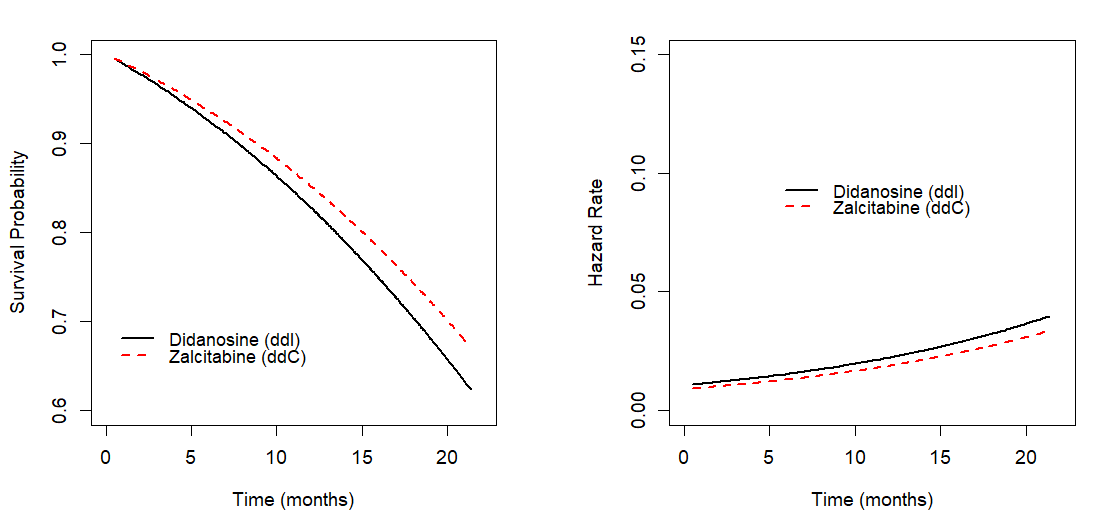
The survival fitting curves based on (7) are provided in Figure 3. The individual fitting curves for four patients are displayed in Figure 4 as an illustrative example. Table 2 presents the posterior results analyzed by BALSAM. Successful MCMC convergence is guaranteed by the result that all values 1.01. The 95% credible interval of , [-0.093, 0.425], and the posterior probability suggests that the two treatments did not demonstrate a significant difference in mortality while adjusting for the other covariates, which is consistent with the results in the Cox model. The posterior mean of , 0.061, and the posterior probability depict strong statistical evidence of an association between the cumulative variation and the hazard. The positive posterior mean and the 95% credible interval suggest that a greater cumulative variation could increase the hazard when adjusting for covariates. The estimated posterior mean of the overall intercept of , , is 7.101. In the CD4 scale, this value translates to 50.42. Thus, the enrolled HIV patients had much lower values of CD4 counts than the normal range. The estimated posterior mean of the overall slope, , is -0.152, coupled with a credible interval [-0.184, -0.120]. This analysis utilizes a linear form to model the longitudinal trajectory of . When the slope is negative, it suggests the overall trend of the CD4 count decreases over time. The 95% credible interval of , [-0.324, 0.696], and the posterior probability suggest the two treatments did not significantly differ in impacting CD4 count. The cumulative variation can be interpreted as the magnitude of CD4 variations here, suggesting a greater CD4 decrease could increase the hazard after adjustment.

| Model Ia (7) Parameters | Mean (SD) | 2.5% | 97.5% | Rhat | ESS |
| Survival Submodel | |||||
| Constant baseline hazard () | 0.009 (0.003) | 0.005 | 0.016 | 1.000 | 17184 |
| Coefficient of treatment () | 0.166 (0.133) | -0.093 | 0.425 | 1.000 | 27000 |
| Coefficient of sex () | -0.376 (0.242) | -0.830 | 0.117 | 1.000 | 11541 |
| Coefficient of AZT () | 0.157 (0.164) | -0.163 | 0.480 | 1.000 | 14917 |
| Coefficient of PreAIDS () | 1.283 (0.225) | 0.855 | 1.734 | 1.000 | 15816 |
| Cumulative Variation | |||||
| Association coefficient () | 0.061 (0.015) | 0.033 | 0.090 | 1.000 | 27000 |
| Longitudinal Submodel | |||||
| Overall mean () | 7.101 (0.256) | 6.595 | 7.599 | 1.000 | 5362 |
| Overall slope () | -0.152 (0.016) | -0.184 | -0.120 | 1.000 | 7367 |
| Coefficient of treatment () | 0.182 (0.259) | -0.324 | 0.696 | 1.001 | 4232 |
| Variance of random error () | 3.016 (0.164) | 2.712 | 3.351 | 1.000 | 27000 |
| Variance of random intercept () | 21.096 (1.520) | 18.300 | 24.275 | 1.000 | 9402 |
| Covariance () | -0.129 (0.075) | -0.280 | 0.015 | 1.000 | 17103 |
| Variance of random slope () | 0.037 (0.006) | 0.026 | 0.050 | 1.000 | 22147 |
Although CD4 count is widely used as a biomarker for treatment progression while studying the efficacy of HIV/AIDS treatments, the CD4 variation and mortality association is not clear yet. Our findings suggest that CD4 cumulative variations significantly impact the hazard, independent of the treatment effect and relevant variables. Targeting CD4 variation may provide an innovative mechanism for new drug development in the future. Furthermore, our findings may help further evaluate CD4 count as a surrogate endpoint instead of overall survival in clinical trials.
5 Discussion
The strengths of BALSAM are featured by the innovative quantification and statistical inference of cumulative variations, which can be embedded in the standard joint models with the shared random effects and cumulative effects. Our model can capture helpful information from longitudinal biomarkers to improve hazard estimation in survival analysis. Cumulative variations assessed by arc length may help identify at-risk or high-risk populations, as illustrated in Figure 5, paving the way for personalized medicine. It can be extended to more types of time-to-event data, including those with competing risks, recurrent events, left censoring, and interval censoring. Our proposed model may be extended to high-dimensional variable selection and latent class procedures. The data-driven time-varying optimal latency window may be explored in BALSAM to accommodate more applications. Besides MCMC algorithms, the Expectation-Maximization (EM) algorithm is often utilized by the MLE approach for joint models. Special care needs to be taken for possible convergence issues as the likelihood increases with each iteration (Dempster et al. 1977).
Our research will have a wide range of applications, including hematology/oncology, cardiology, mental illness, and clinical trials. For instance, it may help identify and compare cancer biomarkers. Adding cumulative variations may help detect abnormal variability of heart rates resulting from diabetes or congestive heart failure. Our methodology may be able to capture mood swings to improve the diagnostic accuracy of mental illness. The signs of elusive diseases, such as Alzheimer’s, may be predicted by monitoring and measuring brain activity. With rapid advancements in wearable devices, real-time data for time-varying health measurements are becoming accessible to everyone. Data variations of these measurements may help optimize mobile health interventions’ design in chronic disease management, personalized medical support, and health recommendations (Nahum-Shani et al. 2018; Lee et al. 2018; Bidargaddi et al. 2020). More exciting applications may include musical composition and speech recognition through arc length to differentiate patterns of sounds and instruments.

SUPPORTING INFORMATION
The computing code and data for the HIV/AIDS clinical trial in Section 4 are available at https://github.com/yangaouic/BALSAM/blob/main/Final_JAGS_CD4_Yan_Gao_26APR2022_GitHub.R.
References
- Abrams et al. (1994) Abrams, D. I., Goldman, A. I., Launer, C., Korvick, J. A., Neaton, J. D., Crane, L. R., Grodesky, M., Wakefield, S., Muth, K., Kornegay, S., et al. (1994). A comparative trial of didanosine or zalcitabine after treatment with zidovudine in patients with human immunodeficiency virus infection. New England Journal of Medicine 330, 657–662.
- Allison (1978) Allison, P. D. (1978). Measures of inequality. American Sociological Review 43, 865–880.
- Alsefri et al. (2020) Alsefri, M., Sudell, M., García-Fiñana, M., and Kolamunnage-Dona, R. (2020). Bayesian joint modelling of longitudinal and time to event data: a methodological review. BMC Medical Research Methodology 20, 94–94.
- Anagnostou et al. (2017) Anagnostou, V., Yarchoan, M., Hansen, A. R., Wang, H., Verde, F., Sharon, E., Collyar, D., Chow, L. Q., and Forde, P. M. (2017). Immuno-oncology trial endpoints: capturing clinically meaningful activity. Clinical Cancer Research 23, 4959–4969.
- Andrieu and Thoms (2008) Andrieu, C. and Thoms, J. (2008). A tutorial on adaptive MCMC. Statistics and Computing 18, 343–373.
- Awoke Ayele et al. (2019) Awoke Ayele, T., Worku, A., Kebede, Y., Zuma, K., Kasim, A., and Shkedy, Z. (2019). Model-based prediction of CD4 cells counts in HIV-infected adults on antiretroviral therapy in Northwest Ethiopia: A flexible mixed effects approach. PLOS One 14, e0218514.
- Battistini Garcia and Guzman (2021) Battistini Garcia, S. A. and Guzman, N. (2021). Acquired Immune Deficiency Syndrome CD4+ Count. StatPearls, Treasure Island, US.
- Bender et al. (2018) Bender, A., Groll, A., and Scheipl, F. (2018). A generalized additive model approach to time-to-event analysis. Statistical Modelling 18, 299–321.
- Bender et al. (2019) Bender, A., Scheipl, F., Hartl, W., Day, A. G., and Küchenhoff, H. (2019). Penalized estimation of complex, non-linear exposure-lag-response associations. Biostatistics 20, 315–331.
- Bender et al. (2005) Bender, R., Augustin, T., and Blettner, M. (2005). Generating survival times to simulate Cox proportional hazards models. Statistics in Medicine 24, 1713–1723.
- Berry et al. (2002) Berry, S. M., Carroll, R. J., and Ruppert, D. (2002). Bayesian smoothing and regression splines for measurement error problems. Journal of the American Statistical Association 97, 160–169.
- Bidargaddi et al. (2020) Bidargaddi, N., Schrader, G., Klasnja, P., Licinio, J., and Murphy, S. (2020). Designing m-health interventions for precision mental health support. Translational Psychiatry 10, 222–222.
- Borst et al. (2018) Borst, J., Ahrends, T., Bąbała, N., Melief, C. J., and Kastenmüller, W. (2018). CD4+ T cell help in cancer immunology and immunotherapy. Nature Reviews Immunology 18, 635–647.
- Briggs et al. (2018) Briggs, W., Cochran, L., Gillett, B., and Schulz, E. (2018). Calculus: early transcendentals (3rd Edition). Pearson, New York, US.
- Brown (2009) Brown, E. R. (2009). Assessing the association between trends in a biomarker and risk of event with an application in pediatric HIV/AIDS. The Annals of Applied Statistics 3, 1163.
- Chołoniewski et al. (2020) Chołoniewski, J., Sienkiewicz, J., Dretnik, N., Leban, G., Thelwall, M., and Hołyst, J. A. (2020). A calibrated measure to compare fluctuations of different entities across timescales. Scientific Reports 10, 1–16.
- Crainiceanu et al. (2005) Crainiceanu, C., Ruppert, D., and Wand, M. P. (2005). Bayesian analysis for penalized spline regression using WinBUGS. Journal of Statistical Software 14,.
- Dafni and Tsiatis (1998) Dafni, U. G. and Tsiatis, A. A. (1998). Evaluating surrogate markers of clinical outcome when measured with error. Biometrics 54, 1445–1462.
- De Gruttola and Tu (1994) De Gruttola, V. and Tu, X. M. (1994). Modelling progression of CD4-lymphocyte count and its relationship to survival time. Biometrics 50, 1003–1014.
- Delgado and Guddati (2021) Delgado, A. and Guddati, A. K. (2021). Clinical endpoints in oncology - a primer. American Journal of Cancer Research 11, 1121.
- Dempster et al. (1977) Dempster, A. P., Laird, N. M., and Rubin, D. B. (1977). Maximum likelihood from incomplete data via the EM algorithm. Journal of the Royal Statistical Society, Series B: Methodology 39, 1–22.
- DeRogatis et al. (2021) DeRogatis, J. M., Viramontes, K. M., Neubert, E. N., and Tinoco, R. (2021). PSGL-1 immune checkpoint inhibition for CD4+ T cell cancer immunotherapy. Frontiers in Immunology 12, 15.
- Desmée et al. (2015) Desmée, S., Mentré, F., Veyrat-Follet, C., and Guedj, J. (2015). Nonlinear mixed-effect models for prostate-specific antigen kinetics and link with survival in the context of metastatic prostate cancer: a comparison by simulation of two-stage and joint approaches. The AAPS Journal 17, 691–699.
- Desmée et al. (2017) Desmée, S., Mentré, F., Veyrat-Follet, C., Sébastien, B., and Guedj, J. (2017). Nonlinear joint models for individual dynamic prediction of risk of death using Hamiltonian Monte Carlo: application to metastatic prostate cancer. BMC Medical Research Methodology 17, 105–105.
- Duane et al. (1987) Duane, S., Kennedy, A., Pendleton, B. J., and Roweth, D. (1987). Hybrid Monte Carlo. Physics Letters B 195, 216–222.
- Fano (1947) Fano, U. (1947). Ionization yield of radiations. II. the fluctuations of the number of ions. Physical Review 72, 26.
- Farkona et al. (2016) Farkona, S., Diamandis, E. P., and Blasutig, I. M. (2016). Cancer immunotherapy: the beginning of the end of cancer? BMC Medicine 14, 1–18.
- Faucett and Thomas (1996) Faucett, C. L. and Thomas, D. C. (1996). Simultaneously modelling censored survival data and repeatedly measured covariates: A Gibbs sampling approach. Statistics in Medicine 15, 1663–1685.
- Feigin (2004) Feigin, A. (2004). Evidence from biomarkers and surrogate endpoints. NeuroRx 1, 323–330.
- Fiore and D’Avolio (2011) Fiore, L. D. and D’Avolio, L. W. (2011). Detours on the Road to Personalized Medicine: Barriers to Biomarker Validation and Implementation. JAMA 306, 1914–1915.
- Fleming and Powers (2012) Fleming, T. R. and Powers, J. H. (2012). Biomarkers and surrogate endpoints in clinical trials. Statistics in Medicine 31, 2973–2984.
- Gasparrini (2014) Gasparrini, A. (2014). Modeling exposure–lag–response associations with distributed lag non-linear models. Statistics in Medicine 33, 881–899.
- Gasparrini et al. (2010) Gasparrini, A., Armstrong, B., and Kenward, M. G. (2010). Distributed lag non-linear models. Statistics in Medicine 29, 2224–2234.
- Gasparrini et al. (2017) Gasparrini, A., Scheipl, F., Armstrong, B., and Kenward, M. G. (2017). A penalized framework for distributed lag non-linear models. Biometrics 73, 938–948.
- Gelfand and Smith (1990) Gelfand, A. E. and Smith, A. F. (1990). Sampling-based approaches to calculating marginal densities. Journal of the American Statistical Association 85, 398–409.
- Gelman and Rubin (1992) Gelman, A. and Rubin, D. B. (1992). Inference from iterative simulation using multiple sequences. Statistical Science 7, 457–472.
- González-Navajas et al. (2021) González-Navajas, J. M., Elkord, E., and Lee, J. (2021). Editorial: CD4 + T cells in cancer immunotherapies. Frontiers in Immunology 12, 737615–737615.
- Guedj (2018) Guedj, J. (2018). Joint modeling of tumor kinetic and overall survival. https://www.fda.gov/media/113417/download.
- Henderson (2002) Henderson, R. (2002). Identification and efficacy of longitudinal markers for survival. Biostatistics 3, 33–50.
- Hoffman and Gelman (2014) Hoffman, M. D. and Gelman, A. (2014). The No-U-Turn sampler: Adaptively setting path lengths in Hamiltonian Monte Carlo. Journal of Machine Learning Research 15, 1593–1623.
- Ibrahim et al. (2001) Ibrahim, J. G., Chen, M., and Sinha, D. (2001). Bayesian survival analysis. Springer series in statistics. Springer, New York, US.
- Ibrahim et al. (2010) Ibrahim, J. G., Chu, H., and Chen, L. M. (2010). Basic concepts and methods for joint models of longitudinal and survival data. Journal of Clinical Oncology 28, 2796–2801.
- Lee et al. (2018) Lee, J.-A., Choi, M., Lee, S. A., and Jiang, N. (2018). Effective behavioral intervention strategies using mobile health applications for chronic disease management: a systematic review. BMC Medical Informatics and Decision Making 18, 12–12.
- Lin et al. (1993) Lin, D., Fischl, M. A., and Schoenfeld, D. (1993). Evaluating the role of CD4-lymphocyte counts as surrogate endpoints in human immunodeficiency virus clinical trials. Statistics in Medicine 12, 835–842.
- MacKay (2003) MacKay, D. J. C. (2003). Information theory, inference, and learning algorithms. Cambridge University Press, Cambridge, UK.
- McCullagh and Nelder (1989) McCullagh, P. and Nelder, A. J. (1989). Generalized linear models (2nd edition). Chapman Hall/CRC, London, UK.
- McCulloch (2003) McCulloch, C. E. (2003). Chapter 4: Generalized linear mixed models (GLMMs), volume 7. Institute of Mathematical Statistics, US.
- Nahum-Shani et al. (2018) Nahum-Shani, I., Smith, S. N., Spring, B. J., Collins, L. M., Witkiewitz, K., Tewari, A., and Murphy, S. A. (2018). Just-in-time adaptive interventions (JITAIs) in mobile health: Key components and design principles for ongoing health behavior support. Annals of Behavioral Medicine 52, 446–462.
- Neal (1993) Neal, R. M. (1993). Probabilistic inference using Markov Chain Monte Carlo methods. University of Toronto, Toronto, CAN.
- Neal (1996) Neal, R. M. (1996). Bayesian learning for neural networks. Springer, New York, US.
- Nesterov (2009) Nesterov, Y. (2009). Primal-dual subgradient methods for convex problems. Mathematical Programming 120, 221–259.
- Pawitan and Self (1993) Pawitan, Y. and Self, S. (1993). Modeling disease market processes in aids. Journal of the American Statistical Association 88, 719–726.
- Redfield and Burke (1988) Redfield, R. R. and Burke, D. S. (1988). HIV infection: The clinical picture. Scientific American 259, 90–99.
- Reeves and Derdeyn (2007) Reeves, J. D. and Derdeyn, C. A. (2007). Entry inhibitors in HIV therapy. Springer, New York, US.
- Robb et al. (2016) Robb, M. A., McInnes, P. M., and Califf, R. M. (2016). Biomarkers and surrogate endpoints: developing common terminology and definitions. JAMA 315, 1107–1108.
- Robert et al. (2018) Robert, P. C., Elvira, V., Tawn, N., and Wu, C. (2018). Accelerating MCMC algorithms. WIREs Computational Statistics 10, e1435.
- Ruppert et al. (2003) Ruppert, D., Wand, M. P., and Carroll, R. J. (2003). Semiparametric regression. Number 12 in Statistical and Probabilistic Mathematics. Cambridge University Press.
- Self and Pawitan (1992) Self, S. and Pawitan, Y. (1992). Modeling a marker of disease progression and onset of disease. In Jewell, N. P., Dietz, K., and Farewell, V. T., editors, AIDS Epidemiology: Methodological Issues, pages 231–255. Birkhäuser Boston, Boston, MA.
- Strimbu and Tavel (2010) Strimbu, K. and Tavel, J. A. (2010). What are biomarkers? Current Opinion in HIV and AIDS 5, 463.
- Sylvestre and Abrahamowicz (2009) Sylvestre, M.-P. and Abrahamowicz, M. (2009). Flexible modeling of the cumulative effects of time-dependent exposures on the hazard. Statistics in Medicine 28, 3437–3453.
- Tsiatis et al. (1995) Tsiatis, A. A., Degruttola, V., and Wulfsohn, M. S. (1995). Modeling the relationship of survival to longitudinal data measured with error. applications to survival and CD4 counts in patients with aids. Journal of the American Statistical Association 90, 27–37.
- U.S. Food and Drug Administration (2021) U.S. Food and Drug Administration (2021). FDA facts: Biomarkers and surrogate endpoints. https://www.fda.gov/about-fda/innovation-fda/fda-facts-biomarkers-and-surrogate-endpoints.
- Wickramarachchi et al. (2014) Wickramarachchi, T. D., Gallagher, C., and Lund, R. (2014). Arc length asymptotics for multivariate time series. Applied Stochastic Models in Business and Industry 31, 264–281.
- Wulfsohn and Tsiatis (1997) Wulfsohn, M. S. and Tsiatis, A. A. (1997). A joint model for survival and longitudinal data measured with error. Biometrics 53, 330–339.
- Zanetti (2015) Zanetti, M. (2015). Tapping CD4 T cells for cancer immunotherapy: the choice of personalized genomics. The Journal of Immunology 194, 2049–2056.
- Zhang et al. (2020) Zhang, J., Pilar, M. R., Wang, X., Liu, J., Pang, H., Brownson, R. C., Colditz, G. A., Liang, W., and He, J. (2020). Endpoint surrogacy in oncology Phase 3 randomised controlled trials. British Journal of Cancer 123, 333–334.
Appendix A
A.1 Observed Joint Likelihood for Model I
The observed joint likelihood for the th subject in Model I is given by
A.2 Observed Joint Likelihood for Model II
The observed joint likelihood for the th subject in Model II is given by
A.3 Computational Challenge
We write our model based on the observed likelihood by integrating out the random effects to reduce the total number of parameters in the MCMC algorithms. This way aims to speed up the posterior estimation by marginalizing over random effects in the likelihood calculation. However, we have to treat a random effect as a parameter in the Bayesian software implementation, resulting in a significant increase in the dimension of parameter space. We conjecture that the posterior estimation of the parameters of interest should be equivalent because the random effects are marginalized eventually in either way. BALSAM revolves around two nested integrals in the cumulative hazard; that is, the upper bound of the inner integral is the variable of the outer in (8). Notably, the inner integral rests on the power of the exponential function. Thus, it is not able to integrate over a region as the classical integration often does for a double or iterated integral. The computation may become complicated when the closed-form solution is not feasible.
| (8) |
The computational challenge results from the sequential order. The ordinary numerical approximation to the integral results in extremely slow convergence if the outer integral has to wait until the inner integral is completed for each time point. Furthermore, the random walk MCMC algorithms require sequential iterations while updating parameters. The likelihood calculation needs to search over all subjects. These sequential iterations require an innovative algorithm strategy. Thus, we adopt a series of efficient algorithms to compute those integrals and accelerate the successful construction of Markov chains, including matrix vectorization, Cholesky decomposition of the covariance matrix, and accelerating MCMC methods.