Towards high temperature holographic superconductors
Abstract
We explore a holographic superconductor model in which a real scalar field is non-minimally coupled to a gauge field. We consider several types of the non-minimal coupling function including exponential, hyperbolic (cosh), power-law and fractional forms. We investigate the influences of the non-minimal coupling parameter on condensation, critical temperature and conductivity. We can categorize our results in two groups. In the first group, conductor/superconductor phase transition is easier to occur for larger values of , while in the second group stronger effects of the non-minimal coupling makes the formation of scalar hair harder. Although the real and imaginary parts of conductivity are impressed by different forms of , they follow some universal behaviors such as connecting with each other through Kramers-Kronig relation in limit or the appearance of gap frequency at low temperatures around which shifts to larger values by increasing the strength of . Among all forms of we observe that gives us better information in wide range of non-minimal coupling constant and temperature. Choosing the best form of , we construct a family of solutions for holographic conductor/superconductor phase transitions to discover the effect of the hyperscaling violation when the gauge and scalar fields are non-minimally coupled. we find that the critical temperature increases for higher effects of hyperscaling violation and non-minimal coupling constant . By increasing these two parameters, we obtain lower values of condensation which means that conductor/superconductor phase transition will acquire easier. Furthermore, we understand that the hyperscaling violation affects the conductivity of the holographic superconductors and changes the expected relation in the gap frequency. Some universal behaviors like infinite DC conductivity are observed.
1 Introduction
Nowadays, we are able to examine the validity of General Relativity (GR) by using observational evidences coming from gravitational waves detections and the first image of the black hole shadow using Event Horizon Telescope (EHT) collaboration [1, 2, 3, 4]. In spite of achieving a lot of success in explaining classical gravitational phenomena, GR is inadequate to explain several problems at the interface between gravitation and high energy physics. In this regards, the physics beyond GR has been arisen to investigate classical and quantum gravity. The motivation is to improve our understanding in different aspects of gravity such as explaining the late-time acceleration of the universe, space-time singularities, dark matter, gravitational waves and inflation epoch [1, 2, 3, 4]. Spontaneous scalarization is a famous notion beyond GR theory. Black hole scalarization is one of the key concepts of holographic superconductors theory due to the spontaneous U(1) symmetry breaking which yields to a phase transition from a black hole with no hair to a hairy one for temperatures below the critical value [5].
Holographic superconductors are constructed based on AdS/CFT duality which is a powerful tool to study strongly correlated systems that relates a weak gravitational system in -dimensions to the strong coupling conformal field theory in -dimensions [6, 5, 7, 8, 9, 10, 11, 12]. The idea of holographic superconductors has attracted a lot of attentions as a theoretical insight to real high temperature superconductors by showing similar behaviors as real supercondutors like second order phase transition [13, 14, 15, 16, 17, 28, 29, 18, 19, 20, 21, 22, 30, 31, 23, 24, 26, 32, 27, 25, 33, 34, 35, 36, 37, 38, 39, 40, 41, 42, 43, 44, 45, 46, 47, 48, 49, 50, 51, 52]. There are still many open problems in strongly coupled systems that each of them can help us to understand the physics of condensed matter systems in this regime. It is worth investigating the effects of the non-minimal coupling on the holographic condensed matter systems. General models for holographic superconductivity parameterized by three couplings which are functions of a real scalar field [53]. It was confirmed that some features are universal and independent of the model such as DC conductivity but important features of the quantum critical behavior strongly depend on the choice of couplings, such as the order of the phase transition and critical exponents of the second-order phase transitions.
In the present work, we concentrate on a modified GR theory dubbed Einstein-Maxwell-Scalar (EMS) theory. We suppose a real scalar field is non-minimally coupled to a gauge field through different forms of coupling functions [54, 55, 56]. Effects of exponential form of the non-minimal coupling function on the phase transition of the holographic superconductors in EMS theory were addressed [56]. Here, we extend the work of [56] by considering different forms of to check how the results depend on the non-minimal coupling function. We solve equations of motion numerically to analyze the influence of the non-minimal coefficient in each kind of coupling function on the critical temperature . Moreover in [53], a phase transition from the second order to the first order appeared in some conditions. Therefore, we explore phase transition of the system to check whether or not different values of in each model of coupling will change the order of phase transition. In [54], spontaneous scalarization for the negative values of the non-minimal coupling term were reported. However, since in holographic setup the formation of scalar hair appears by going down the temperatures below the critical value, we consider positive values of , too. By applying an appropriate electromagnetic perturbation on the black hole background, we explore the behavior of the real and imaginary parts of conductivity for different values of in each form of . We would like to explore how the universal relation between the gap frequency and critical temperature in holographic setup, , can be changed based on different choices of the non-minimal component.
Asymptotically AdS geometry corresponds to relativistically conformal theory in the boundary but the condensed matter theory is non-relativistic in most cases. Therefore, it is interesting to generalize the holographic superconductor models to nonrelativistic situations by using the nonrelativistic version of AdS/CFT correspondence. This is achieved in Lifshitz-like geometry with dynamical exponent in which the time scales different from the space, which is similar to the behavior of the condensed matter systems near the quantum critical point and brings some new features of holographic superconductor models (see e.g. [57, 58, 59, 60, 61, 62, 63] and references therein). On the other side, hyperscaling violation metric, as an extension of the Lifshitz metric, has grabbed a lot of attentions because of its potential to describe holographically the realistic condensed matter systems [64, 65, 66, 67, 68, 69]. We shall also construct solutions of the holographic superconductors in the background of the hyperscaling violation black hole when gauge and scalar fields are non-minimally coupled. We employ the numerical method to analyze the influences of the hyperscaling violating parameter, , and the non-minimal coupling parameter, , on the condensation, critical temperature and conductivity of the system. In [67], it was mentioned that by increasing , the critical temperature increases analytically but first decreases and then increases numerically. Therefore, the behavior of the critical temperature due to various values of and should be checked. Moreover, the second order phase transition is one of main concepts of superconductors. We will check whether or not the order of phase transition will differ by applying different strength of and . In addition, we will study the electrical conductivity in holographic setup to check the universal behaviors of conductivity like infinite Dc conductivity and .
This paper is organized as follows. In section 2, we introduce the holographic model when scalar and gauge fields are non-minimally coupled via different forms of the coupling functions. Then, we analyze condensation and critical temperature of -dimensional holographic superconductor impressed by various strength of non-minimal coupling constant for each model. After that we investigate the role of the non-minimal coupling on the real and imaginary parts of conductivity. Next in 3, we present the holographic setup with hyperscaling violation by studying the behavior of condensation, critical temperature and conductivity. Finally in section 4, we summarize our results.
2 Holographic Setup
The action of the four dimensional gravity in the presence of a real scalar field with mass and charge which is non-minimally coupled to the Maxwell gauge field is given by [54, 55, 56],
| (2.1) |
where , and represent metric determinant, Ricci scalar and the curvature radius of AdS spacetime, respectively. In the above action stands for the gauge field that connects to the electromagnetic field strength tensor through . denotes the non-minimal coupling of the scalar field and Maxwell background which has various coupling choices. In this work we will consider some forms of non-minimal coupling function with as the coupling constant as below [54, 55, 56]
for , we have
| (2.2) | |||
| (2.3) |
In the probe limit when the scalar and electromagnetic fields do not backreact, the metric of a planar Schwarzschild-AdS black hole has the following form [5]
| (2.4) | |||
| (2.5) |
with as the horizon location. The Hawking temperature of the black hole is given by [5]
| (2.6) |
without loss of generality, we set for the rest of this work.
Condensation of the scalar field
We can obtain the equations of motion by varying the action (2.1) with respect to scalar field and gauge field as
| (2.7) | |||
| (2.8) |
where . Choosing and yields to
| (2.9) |
| (2.10) |
in which primes denote the derivatives with respect to the radial coordinate . If we consider and as chemical potential and charge density, the above equations have the asymptotic behavior() as
| (2.11) | |||
| (2.12) |
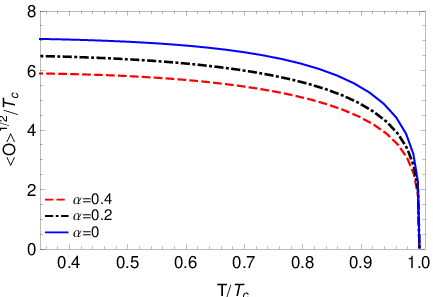
In this work, we take and . Since we are looking for spontaneous phase transition, we set which means the condensate turns on without being sourced. plays the role of expectation value of the order parameter . The effect of different values of coupling constant and various coupling functions on critical temperature and condensation, can be obtained by solving equations (2.9) and (2.10) numerically by applying shooting method. The results of critical temperatures are listed in table 1. Based on these outcomes, increasing the effect of non-minimal coupling in group 2(HCos, Exp(+) and P(+) cases) leads to higher values of critical temperature while in group 1(F, Exp(-) and P(-) cases) we face with difficulty in formation of scalar hair. In addition, the trend of condensation as a function of temperature for different strength of non-minimal coupling constants in various coupling forms are shown in figure 1. As said before, condensation values follow different trends due to increasing the values of for group 2 in comparison with group 1. Conductor/superconductor phase transition is easier to form for larger values of in group 2 by diminishing the values of condensation. Group 1 functions can not give us information about low temperatures limit by increasing the values of because of numerical solution limitations. However, we can follow numerical solution for and even larger values in P(+) case. Our choice of non-minimal coupling function is not so clear on the values of critical temperature and we have two groups of answer which is reasonable based on equations (2.2) and (2.3) for and we expect various results of critical temperature for each case by increasing the values of . However, running our numerical code for stronger effects of depends critically on our choice of . For example, we can follow our numerical calculation just up to in group 1 while in group 2 it is so clear that each forms of allows us to obtain results up to a specific value of non-minimal coupling constant. Furthermore, in all cases we face second order phase transition.
| group 1 | group 2 | |||||
| Exp(-) | F | P(-) | Exp(+) | HCos | P(+) | |



Conductivity
Electrical conductivity in holographic setup can be obtained by applying an appropriate perturbation as on the black hole background which yields to
| (2.13) |
and behaves asymptotically as
| (2.14) |
by considering and as constant parameters, asymptotic solution of is
| (2.15) |
so, the electrical conductivity can be evaluated as
| (2.16) |
Behavior of real and imaginary parts of conductivity as a function of is shown in figures 2-6 for different values of nonminimal coupling in various forms of . In general figures follow some universal trends. For example at low frequency regime, real and imaginary parts of conductivity are related to each other via Kramers-Kronig relation by having a delta and pole respectively. However, at high frequency limit, both parts of conductivity tend to a constant value. We observe the appearance of gap frequency at low temperatures which shifts to higher values of by increasing the strength of non-minimal coupling from to which is much larger than the BCS prediction due to strong coupling nature of high temperature superconductors. Because of difficulty in numerical solution of P(-) and F cases, we can not obtain their behavior of conductivity at . Meanwhile, the trend of conductivity in F case is far different from other models.


3 Holographic setup with hyperscaling violation
In order to study the effect of hyperscaling violation on the holographic superconductors, the black hole solution with hyperscaling violation reads [64, 68]
| (3.1) |
where
| (3.2) |
with , and as the radius of the event horizon, dynamical exponent and hyperscaling violation exponent, respectively. Therefore, the Hawking temperature is given by [68]
| (3.3) |
We concentrate on probe limit because it can simplify the problem but retain most of the interesting physics. At the asymptotic limit and , the metric reduces to [68]
| (3.4) |
this is the most general geometry which is spatially homogeneous and covariant under the following scale transformations [68]
| (3.5) |
in which it is obvious that for non-zero values of , the distance is not invariant under the scaling which in the context of AdS/CFT indicates violations of hyperscaling in the dual field theory [68]. Evidently when and , it reduces to the pure Lifshitz case [57]. In this work, we focus on , . Observations indicate that backgrounds whose asymptotic behavior coincides with the above metric may be of interest to condensed matter physics. Therefore, studying AdS/CFT correspondence in this case is valuable.
Condensation of scalar field
In the probe limit, we will construct the holographic superconductors when a real scalar field coupled non-minimally to the electromagnetic gauge field in the background of the hyperscaling violation black hole as equation (2.1) [54, 55, 56] with . We obtain the equations of motion by varying the action with respect to gauge field and scalar field and taking the ansatz of the matter fields as and
| (3.6) |
| (3.7) |
which have asymptotic behavior as [67]
| (3.8) |
| (3.9) |
Same as previous section by applying shooting method, we study the effect of different values of hyperscaling term and non-minimal coupling constant by solving equations (3.6) and (3.7) numerically. We choose . In table II, the consequences of different choices of and in critical temperature are listed. Based on our results, increasing each of these parameters makes conductor/superconductor phase transition easier to form by increasing the critical temperature. In addition, the effects of the hyperscaling violation on the condensation of the scalar operators is shown in figure 7 which prove the outcomes of critical temperature. In all cases for higher effects of hyperscaling and non-minimal terms, condensation values go down. Moreover, for all cases considered here, the condensation is single-valued near the critical temperature and the condensate drops to zero continuously at the critical temperature. Fitting these curves, we obtain a square root behavior for small condensate which means that the phase transition belongs to the second order and the critical exponent of the system takes the mean-field value 1/2.


Except when , the critical temperature first goes down and then goes up by increasing .
Conductivity
Now, we want to explore the conductivity of holographic superconductors with the hyperscaling violation when gauge and scalar fields couple to each other non-minimally. So, the equation of motion for , due turning on a perturbation same as in the previous section, is given by
| (3.10) |
which asymptotically behaves as
| (3.11) |
based on the AdS/CFT dictionary, the electrical conductivity equals to
| (3.12) |
By following the numerical approach, behavior of real and imaginary parts of conductivity as a function of are shown in figures 8 and 9. the non-minimal coupling and the hyperscaling violation really affect the conductivity of the holographic superconductors. However, real and imaginary parts follow some universal behavior. For instance based on these figures, in high frequency regimes, real and imaginary parts of conductivity approach to a constant value based on our choice of and . Near the zero frequency region, a delta function is contained in the real part of the conductivity as which indicates infinite DC conductivity. While there exists a pole in the imaginary part and it diverges . At low frequency region, real and imaginary parts are connected to each other via Kramers-Kronig relation. In addition, for all cases considered here according to figures 10 and 11, we observe that the gap frequency shifts to higher frequencies when we increase the value of and which means increasing the effect of the hyperscaling violation and non-minimal coupling changes the universal relation in the gap frequency . larger values of and make the gap frequency flatter.


4 Conclusion and Remarks
First of all, we studied holographic superconductors in the EMS model by considering different types of non-minimal coupling of scalar and gauge fields including an exponential, a hyperbolic (cosh), a power-law and a fractional coupling forms. We solved the field equations numerically with the help of shooting method and disclose the effects of different values of the non-minimal coupling on the critical temperature and condensation for each form of . The effects of different values of on critical temperature and condensation is not so obvious and we obtain two groups of answers. It’s reasonable because they have the same Taylor expansion for . According to our results, we have superconductors in higher temperatures for group 2 by increasing the values of . While we see completely different behavior in group 1 for stronger effects of and conductor/superconductor phase transition will face with more difficulty to occur. In addition, we have problem in numerical code in for lower temperatures in group 1. The condensation values follow the same trend as critical temperature by increasing the strength of non-minimal coupling. Moreover, we found out that different choices for and do not change the order of phase transition. In addition, we analyze the electrical conductivity by turning on a suitable perturbation on black hole background which corresponds to electrical current in CFT part. While various coupling functions follow different behavior for conductivity, almost all figures show some universal trends. For instance in limit, the real parts of conductivity show a delta trend while the imaginary parts have a pole and these two parts are connected to each other via Kramers-Kronig relation. However at high frequency regime, both parts tend to a constant value. Furthermore, a gap frequency forms at low temperatures at about which shifts to higher values by increasing the effect of non-minimal coupling. Therefore, we understood that certain properties of superconductors like DC conductivity and spontaneous symmetry breaking are universal and do not depend on the model. Due to numerical calculation limitations, we can not study the behavior of conductivity at low temperatures in some forms of . In order to sum up, we should say that among all forms of non-minimal coupling functions that we studied in this work, gives us more information about different values of at a wide range of temperature.
Secondly, from the perspective of application to realistic systems, it is of certain interests to explore the effects of dynamical exponent and hyperscaling violation on the holographic superconductors. Therefore, we also have considered a holographic superconductor model in EMS theory with a hyperscaling violating term. At the first step, we studied the effect of different choices of non-minimal coupling constant and hyperscaling violation term on condensation and critical temperature numerically. Based on our results, increasing the effect of or makes conductor/superconductor phase transition easier to form by increasing temperature and decreasing condensation. Due to square root behavior of condensate, the critical exponent of the system takes the mean-field value 1/2 in all cases. In the next step, we analyze the electrical conductivity in holographic setup by applying an appropriate perturbation on the black hole background. Our choice of and have a great impact on the shape of real and imaginary parts of conductivity. However, they follow some universal approaches, too.
References
- [1] A. Bryant, H. O. Silva, K. Yagi and K. Glampedakis, Eikonal quasinormal modes of black holes beyond general relativity III: scalar Gauss-Bonnet gravity, Phys. Rev. D 104, 044051 (2021) [arXiv:2106.09657 [gr-qc]].
- [2] P. Wagle, N. Yunes and H. O. Silva, Quasinormal modes of slowly-rotating black holes in dynamical Chern-Simons gravity, Phys. Rev. D 105, 124003 (2022) [arXiv:2103.09913 [gr-qc]].
- [3] C. F. B. Macedo, J. Sakstein, E. Berti, L.Gualtieri, H. O. Silva and T. P. Sotiriou, Self-interactions and Spontaneous Black Hole Scalarization, Phys. Rev. D 99, 104041 (2019) [arXiv:1903.06784 [gr-qc]].
- [4] C. A. R. Herdeiro, E. Radu, H. O. Silva, T. P. Sotiriou and Nicolás Yunes, Spin-induced scalarized black holes, Phys. Rev. Lett. 126, 011103 (2021) [arXiv:2009.03904 [gr-qc]].
- [5] S. A. Hartnoll, C. P. Herzog and G. T. Horowitz, Building a Holographic Superconductor, Phys. Rev. Lett. 101, 031601 (2008) [arXiv:0803.3295 [hep-th]].
- Maldacena. [1998] J. M. Maldacena, The Large N Limit of Superconformal Field Theories and Supergravity, Adv. Theor. Math. Phys. 2, 231 (1998) [arXiv:hep-th/9711200v3].
- Gubser et al. [1998] S. S. Gubser, I. R. Klebanov and A. M. Polyakov, Gauge Theory Correlators from Non-Critical String Theory, Phys. Lett. B 428, 105 (1998) [arXiv:hep-th/9802109].
- Witten et al. [1998] E. Witten, Anti De Sitter Space And Holography, Adv. Theor. Math. Phys. 2, 253 (1998) [arXiv:hep-th/9802150].
- Horowitz et al. [2008] G. T. Horowitz and M. M. Roberts, Holographic superconductors with various condensates, Phys. Rev. D 78, 126008 (2008) [arXiv:0810.1077 [hep-th]].
- Ren. [2010] J. Ren, One-dimensional holographic superconductor from correspondence, JHEP 1011, 055 (2010) [arXiv:1008.3904[hep-th]].
- Horowitz [2011] G. T. Horowitz, Introduction to Holographic Superconductors, Lect. Notes Phys. 828 , 313 (2011) [arXiv:1002.1722[hep-th]].
- Hartnoll [2009] S. A. Hartnoll, Lectures on holographic methods for condensed matter physics, Class. Quantum Grav. 26, 224002 (2009) [arXiv:0903.3246[hep-th]].
- Herzog. [2009] C. P. Herzog, Lectures on Holographic Superfluidity and Superconductivity, J. Phys. A 42, 343001 (2009) [arXiv:0904.1975[hep-th]].
- Gubser. [2009] S. S. Gubser, C. P. Herzog, S. S. Pufu and T. Tesileanu, Superconductors from superstrings, Phys. Rev. Lett. 103, 141601 (2009) [arXiv:0907.3510[hep-th]].
- HHH. [2008] S. A. Hartnoll, C. P. Herzog and G. T. Horowitz, Holographic Superconductors, JHEP 0812, 015 (2008) [arXiv:0810.1563[hep-th]].
- Jing ,Chena [210] J. Jing, S. Chen, Holographic superconductor in the Boren-Infeld electrodynamics, Phys. Lett. B 686, 68 (2010) [arXiv:1001.4227[gr-qc]].
- cai [2015] R. G. Cai, L. Li, Li-Fang Li, Run-Qiu Yang, Introduction to holographic superconductor models, Sci China Phys. Mech. Astron. 58, 060401 (2015) [arXiv:1502.00437[hep-th]].
- Ge [2010] X. H. Ge, B. Wang, S. F. Wu, and G. H. Yang, Analytical study on holographic superconductors in external magnetic field, JHEP 1008, 108 (2010) [arXiv:1002.4901[hep-th]].
- Ge [2012] X. H. Ge, S. F. Tu, B. Wang, -Wave holographic superconductors with backreaction in external magnetic fields, JHEP 09, 088 (2012) [arXiv:1209.4272[hep-th]].
- Kuang [2013] X. M. Kuang, E. Papantonopoulos, G. Siopsis, B. Wang, Building a Holographic Superconductor with Higher-derivative Couplings, Phys. Rev. D 88, 086008 (2013) [arXiv:1303.2575[hep-th]].
- Pan [2011] Q. Pan, J. Jing, B. Wang, Analytical investigation of the phase transition between holographic insulator and superconductor in Gauss-Bonnet gravity, JHEP 11, 088 (2011) [arXiv:1105.6153 [gr-qc]].
- CAI [11] R. G. Cai, H. F Li, H.Q. Zhang, Analytical Studies on Holographic Insulator/Superconductor Phase Transitions, Phys. Rev. D 83, 126007 (2011) [arXiv:1103.5568 [hep-th]].
- cai [10] R. G. Cai, Z.Y. Nie, H.Q. Zhang, Holographic p-wave superconductors from Gauss-Bonnet gravity, Phys. Rev. D 82, 066007 (2010) [arXiv:1007.3321 [hep-th]].
- yao [2013] W. Yao, J. Jing, Analytical study on holographic superconductors for Born-Infeld electrodynamics in Gauss-Bonnet gravity with backreactions, JHEP 1305, 101 (2013) [arXiv:1306.0064[gr-qc]].
- [25] S. Gangopadhyay, D. Roychowdhury, Analytic study of properties of holographic superconductors in Born-Infeld electrodynamics, JHEP 05, 002 (2012) [arXiv:1201.6520[hep-th]]
- [26] Z. Zhao, Q. Pan, S. Chen and J. Jing, Notes on holographic superconductor models with the nonlinear electrodynamics, Nucl. Phys. B 871, 98 (2013) [arXiv:1212.6693[hep-th]].
- [27] Y. Liu, Y. Gong and B. Wang, Non-equilibrium condensation process in holographic superconductor with nonlinear electrodynamics, JHEP 1602, 116 (2016) [arXiv:1505.03603[hep-ph]].
- Sheykhi et al. [2016] A. Sheykhi, H. R. Salahi, A. Montakhab, Analytical and Numerical Study of Gauss-Bonnet Holographic Superconductors with Power-Maxwell Field, JHEP 1604, 058 (2016) [arXiv:1603.00075[gr-qc]].
- SHsh [17] A. Sheykhi, F. Shaker, Effects of backreaction and exponential nonlinear electrodynamics on the holographic superconductors, Int. J. Mod. Phys. D 26, 1750050 (2017) [arXiv:1606.04364[gr-qc]].
- SHSH [16] A. Sheykhi, F. Shaker, Analytical study of properties of holographic superconductors with exponential nonlinear electrodynamics, Can. J. of Phys. 94, 1372 (2016) [arXiv:1601.05817[hep-th]].
- [31] A. Sheykhi, F. Shaker, Analytical study of holographic superconductor in Born-Infeld electrodynamics with backreaction, Phys Lett. B 754, 281 (2016) [arXiv:1601.04035[hep-th]].
- [32] S. I. Kruglov, Holographic superconductor with nonlinear arcsin-electrodynamics, Annalen Phys 530, 1800070 (2018) [arXiv:1801.06905[hep-th]].
- [33] M. Mohammadi, A. Sheykhi and M. Kord Zangeneh, Analytical and numerical study of backreacting one-dimensional holographic superconductors in the presence of Born-Infeld electrodynamics, Eur. Phys. J. C 78, 654 (2018) [arXiv:1805.07377[hep-th]].
- BCS [1957] J. Bardeen, L. N. Cooper, J. R. Schrieer, Theory of Superconductivity, Phys. Rev. 108, 1175 (1957).
- [35] A.P. Mackenzie, Y. Maeno, Lectures on holographic methods for condensed matter physics, Physica B 280, 148 (2000).
- [36] R.-G. Cai, S. He, L. Li, and L.F. Li, A Holographic Study on Vector Condensate Induced by a Magnetic Field, JHEP 1312, 036 (2013) [arXiv:1309.2098 [hep-th]].
- [37] R.G.Cai, L. Li, L.F. Li, A Holographic -wave Superconductor Model, JHEP 1401, 032 (2014) [arXiv:1309.4877[hep-th]].
- [38] A. Donos and J.P. Gauntlett, Holographic helical superconductors, JHEP 12, 091 (2011) [arXiv:1109.3866 [hep-th]].
- [39] S. S. Gubser and S. S. Pufu, The Gravity dual of a -wave superconductor, JHEP, 0811, 033 (2008) [arXiv:0805.2960 [hep-th]].
- [40] P. Chaturvedi, G. Sengupta, -wave Holographic Superconductors from Born-Infeld Black Holes, JHEP 1504, 001 (2015) [arXiv:1501.06998 [hep-th]].
- [41] M. M. Roberts and S. A. Hartnoll, Pseudogap and time reversal breaking in a holographic superconductor, JHEP 0808, 035 (2008) [arXiv:0805.3898[hep-th]].
- [42] H. B. Zeng, W. M. Sun and H. S. Zong, Supercurrent in p-wave Holographic Superconductor, Phys. Rev. D 83, 046010 (2011) [arXiv:1010.5039 [hep-th]].
- [43] R. G. Cai, Z. Y. Nie and H. Q. Zhang, Holographic Phase Transitions of P-wave Superconductors in Gauss-Bonnet Gravity with Back-reaction, Phys. Rev. D 83, 066013 (2011) [arXiv:1012.5559[hep-th]].
- [44] L. A. Pando Zayas and D. Reichmann, A Holographic Chiral Superconductor, Phys. Rev. D 85, 106012 (2012) [arXiv:1108.4022[hep-th]].
- [45] D. Momeni, N. Majd and R. Myrzakulov, -wave holographic superconductors with Weyl corrections, Europhys. Lett. 97, 61001 (2012) [arXiv:1204.1246[hep-th]].
- [46] M. Mohammadi, A. Sheykhi and M. Kord Zangeneh, One-dimensional backreacting holographic -wave superconductors, Eur. Phys. J. C 78, 984 (2018) [arXiv:1901.10540[hep-th]].
- [47] F. Benini, C. P. Herzog, R. Rahman and A. Yarom, Gauge gravity duality for d-wave superconductors: prospects and challenges, JHEP 1011, 137 (2010) [arXiv:1007.1981[hep-th]].
- [48] F. Benini, C. P. Herzog and A. Yarom, Holographic Fermi arcs and a -wave gap, Phys. Lett. B 701, 626 (2011) [arXiv:1006.0731[hep-th]].
- [49] M. Mohammadi, A. Sheykhi, Lifshitz scaling effects on the holographic -wave superconductors coupled to nonlinear electrodynamics, Eur. Phys. J. C 80, 928 (2020) [arXiv:2010.07105 [hep-th]].
- [50] M. Mohammadi, A. Sheykhi, Conductivity of the one-dimensional holographic -wave superconductors in the presence of nonlinear electrodynamics, Phys. Rev. D 100, 086012 (2019) [arXiv:1910.06082 [hep-th]].
- [51] M. Mohammadi and A. Sheykhi, Conductivity of the holographic p-wave superconductors with higher order corrections, Eur. Phys. J. C 79, 743 (2019) [arXiv:1908.07992 [hep-th]].
- [52] M. Mohammadi, A. Sheykhi, Gauss-Bonnet holographic superconductors in lower-dimensions, Eur. Phys. J. Plus 137, 852 (2022) [arXiv:2202.03048 [hep-th]].
- [53] F. Aprile, J. G. Russo, Models of Holographic superconductivity, Phys. Rev. D 81, 026009 (2010) [arXiv:0912.0480v2 [hep-th]].
- [54] P. G. S. Fernandes, C. A. R. Herdeiro, A. M. Pombo, E. Radu and N. Sanchis-Gual, Spontaneous scalarisation of charged black holes: coupling dependence and dynamical features, Class. Quantum Grav. 36 134002 (2019) [arXiv:1902.05079 [gr-qc]].
- [55] Y. S. Myung and D. C. Zou, Stability of scalarized charged black holes in the Einstein-Maxwell-Scalar theory, Eur. Phys. J. C 79,641 (2019) [arXiv:1904.09864 [gr-qc]].
- [56] Y. Chen, X. Guo and P. Wang, Holographic Superconductors in a Non-minimally Coupled Einstein-Maxwell-scalar Model [arXiv:2111.03810 [hep-th]].
- [57] J. W. Lu, Y. B Wu, P. Qian, Y. Y. Zhao, X. Zhang, N. Zhang, Lifshitz Scaling Effects on Holographic Superconductors, Nucl. Phys. B 887, 112 (2014) [arXiv:1311.2699v4].
- [58] M. Natsuume and T. Okamura, Holographic Lifshitz superconductors: Analytic solution, Phys. Rev. D 97, 066016 (2018) [arXiv:1801.03154].
- [59] Z. Sherkatghanad, B. Mirza, F. Lalehgani Dezaki, Exponential nonlinear electrodynamics and backreaction effects on Holographic superconductor in the Lifshitz black hole background, Int. J. Mod. Phys. D 26, 1750175 (2017) [arXiv:1708.04289].
- [60] Z. Zhao, Q. Pan, J. Jing, Notes on analytical study of holographic superconductors with Lifshitz scaling in external magnetic field, Phys. Lett. B 735 , 438 (2014) [arXiv:1311.6260].
- [61] E. Brynjolfsson, U. H. Danielsson, L. Thorlacius, and T. Zingg, Holographic superconductors with Lifshitz scaling, J. Phys. A 43, 065401 (2010) [arXiv: 0908.2611 [hep-th]].
- [62] S.J. Sin, S.S. Xu, and Y. Zhou, Holographic superconductor for a Lifshitz fixed point, Int. J. Mod. Phys. A 26, 4617 (2011) [arXiv: 0909.4857 [hep-th]].
- [63] Y.Y. Bu, Holographic superconductors with z=2 Lifshitz scaling, Phys. Rev. D 86, 046007 (2012) [ arXiv:1211.0037 [hep-th]].
- [64] C. Charmousis, B. Gouteraux, B. S. Kim, E. Kiritsis and R. Meyer, Holographic The- ories for low-temperature condensed matter systems, JHEP 1011, 151 (2010) [arXiv:1005.4690 [hep-th]].
- [65] X. Dong, S. Harrison, S. Kachru, G.Torroba and H.Wang, Aspects of holography for theories with hyperscaling violation, JHEP 06 (2012) 041 [arXiv:1201.1905v4[hep-th]].
- [66] Z.Y. Fan, Holographic superconductors with hyperscaling violation, JHEP 1309, 048 (2013)[arXiv:1305.2000 [hep-th]].
- [67] Q. Pan, S. J. Zhang, Revisiting holographic superconductors with hyperscaling violation, Eur. Phys. J. C 76, 126 (2016) [arXiv:1510.09199 [hep-th]].
- [68] M. Alishahiha, E. Ó Colgáin, H. Yavartanoo ,Charged Black Branes with Hyperscaling Violating Factor, JHEP 2012, 137 (2012) [ arXiv:1209.3946 [hep-th]].
- [69] S. Zhang, Z. Zhao, Q. Pan and J. Jing ,Excited states of holographic superconductors with hyperscaling violation, Nucl. Phys. B 976, 115701(2022) [arXiv:2107.09486 [hep-th]].