Impact of Mgii interstellar medium absorption on near-ultraviolet exoplanet transit measurements2021Impact of Mgii interstellar medium absorption on near-ultraviolet exoplanet transit measurements–14
Abstract
Ultraviolet (UV) transmission spectroscopy probes atmospheric escape, which has a significant impact on planetary atmospheric evolution. If unaccounted for, interstellar medium absorption (ISM) at the position of specific UV lines might bias transit depth measurements, and thus potentially affect the (non-)detection of features in transmission spectra. Ultimately, this is connected to the so called “resolution-linked bias” (RLB) effect. We present a parametric study quantifying the impact of unresolved or unconsidered ISM absorption in transit depth measurements at the position of the Mgii h&k resonance lines (i.e. 2802.705 Å and 2795.528 Å, respectively) in the near-ultraviolet spectral range. We consider main-sequence stars of different spectral types and vary the shape and amount of chromospheric emission, ISM absorption, and planetary absorption, as well as their relative velocities. We also evaluate the role played by integration bin and spectral resolution. We present an open-source tool enabling one to quantify the impact of unresolved or unconsidered Mgii ISM absorption in transit depth measurements. We further apply this tool to a few already or soon to be observed systems. On average, we find that ignoring ISM absorption leads to biases in the Mgii transit depth measurements comparable to the uncertainties obtained from the observations published to date. However, considering the bias induced by ISM absorption might become necessary when analysing observations obtained with the next generation space telescopes with UV coverage (e.g. LUVOIR, HABEX), which will provide transmission spectra with significantly smaller uncertainties compared to what obtained with current facilities (e.g. HST).
Keywords:
stars – ultraviolet – Planet-star interactions – Stellar activity – late-type stars1 Introduction
Atmospheric escape is one of the key processes affecting the long-term evolution of a planetary atmosphere and it plays a pivotal role in shaping the currently observed exoplanet population (Lecavelier Des Etangs 2007; Lopez & Fortney 2013; Owen & Wu 2017; Jin & Mordasini 2018; Kubyshkina et al. 2018, e.g.). The first detection of exoplanet atmospheric escape occurred through Ly transmission spectroscopy (Vidal-Madjar et al. 2003). Since then, this technique has been central in observationally probing upper atmospheres and escape (Lecavelier des Etangs et al. 2012; Ehrenreich et al. 2015; Bourrier et al. 2018, e.g.). One of the most significant problems of Ly transmission spectroscopy is that, because of interstellar medium (ISM) absorption, Ly transit observations are possible only for nearby stars, typically within 50 pc (Ehrenreich et al. 2012, e.g.). Furthermore, even for stars for which Ly transmission spectroscopy is possible, the observations typically probe high velocity neutral hydrogen, because the core of the line, which is where most of the planetary absorption is located, is often (fully) absorbed by neutral hydrogen in the ISM (Guinan et al. 2016; Bourrier et al. 2017).
Transmission spectroscopy observations aiming at studying atmospheric escape have also been conducted at near-ultraviolet (NUV) wavelengths. This is to gain from the higher NUV stellar flux, compared to the far-ultraviolet (FUV), but also to gain from the fact that in the NUV the stellar emission is more temporally stable and spatially homogeneous (Haswell 2010; Haswell et al. 2012). Just a few exoplanets have been observed in the NUV from space using either spectroscopy or broad-band photometry (Fossati et al. 2010; Haswell et al. 2012; Vidal-Madjar et al. 2013; Salz et al. 2019; Sing et al. 2019; Cubillos et al. 2020; Wakeford et al. 2020; Lothringer et al. 2022). The NUV spectral range is dominated by a plethora of strong lines of several metals, with the most dominant being Mg and Fe. The most prominent NUV spectral features are the Mgii h&k resonance lines at 2800 Å. In late-type stars, these lines present a core reversal (i.e. emission) that originates in the chromosphere and transition region (Hall 2008; Youngblood et al. 2022, e.g.). Because these are resonance lines, Mg is a rather abundant element, and singly ionised Mg is the most abundant Mg ion in the ISM (Frisch & Slavin 2003, e.g.), stellar emission at the core of these lines is affected by ISM absorption, similarly to Ly, though typically less pronounced. Indeed, ISM Mgii absorption lines have been ubiquitously found in the NUV spectra of stars, regardless of their distance from Earth (Redfield & Linsky 2002, e.g.).
Similar to the Ly line, in systems hosting transiting planets with an extended atmosphere, depending on the radial velocity of the ISM cloud with respect to that of the star, the Mgii ISM absorption features may lie on top of the planetary absorption features. If this ISM absorption, which occurs after the planetary atmosphere has imprinted its signature in the stellar flux, is unaccounted for, the transmission spectrum at the core of the Mgii lines might be biased. This is the case of broad band photometry, but it may occur also with transmission spectroscopy, for example if the low signal-to-noise ratio of the data requires binning and/or does not enable one to resolve the ISM absorption features. As shown below (Section 3), this occurs as a result of the different shape of the stellar, planetary absorption, and ISM absorption features, despite that of the transit depth is a differential measurement and the impact of ISM absorption cancels out when considering a single wavelength point. The origin of this phenomenon is similar to the one that Deming & Sheppard 2017 called “resolution-linked bias” (RLB).
The most representative case is certainly that of the WASP-12 system. The late F-type star WASP-12 hosts a hot Jupiter with an orbital period of about 1 day (Hebb et al. 2009). Fossati et al. 2010 , Haswell et al. 2012 and Nichols et al. 2015 presented the results of HST/COS NUV transmission spectroscopy observations of WASP-12b that also covered the Mgii h&k lines. The observations indicated that the planet hosts an escaping atmosphere that is rich in metals as heavy as iron. The COS spectra revealed that, surprisingly, the core of the Mgii lines does not show any reversal, which has been explained by a combination of ISM absorption and absorption local to the system caused by a cloud of planetary escaped material surrounding the star (Haswell et al. 2012; Fossati et al. 2013; Debrecht et al. 2018; Dwivedi et al. 2019). Furthermore, the large distance to the star (Gaia Collaboration et al. 2018, 430 pc;) implied that, to gather enough signal for significantly detecting the planet and its atmospheric signature, the data needed to be heavily rebinned, integrating across about 20 Å on either side of the Mgii lines. Therefore, the transit depth measured in the region of the Mgii h&k lines might have been biased by the unresolved ISM absorption.
WASP-121b and HD209458b have also been observed employing NUV HST/STIS transmission spectroscopy covering the Mgii h&k lines (Sing et al. 2019; Vidal-Madjar et al. 2013; Cubillos et al. 2020). Despite the higher signal-to-noise of the data, compared to that of WASP-12b, which enabled resolving the ISM absorption features on top of the chromospheric stellar emission, the analysis had been carried out integrating the flux in the line cores without excluding the regions affected by the ISM absorption. This may have biased the transmission spectra around the line cores.
There is therefore the need to identify, and eventually quantify, the impact of unresolved or unconsidered ISM absorption in the core of the Mgii lines in transit depth measurements. To this end, we employ synthetic spectra and take into account a number of stellar, planetary, ISM, instrumental, and analysis parameters. Furthermore, we present an open-source code enabling one to estimate the correction to the transit depth caused by the unresolved or unconsidered ISM absorption. This work is organised as follows. In Sections 2 and 3, we present the input parameters and the analysis methods. In Section 4, we show the results, which we discuss in Section 5. We gather the conclusions in Section 6.
2 Input parameters

We employ synthetic spectra to quantify the impact of unresolved ISM absorption at the position of the Mgii h&k resonance lines in planetary transit measurements. We build up the synthetic spectra by adding the ISM and planetary absorption and line emission features on top of the photospheric spectra, thus enabling us to control each relevant physical parameter. Furthermore, we consider also instrumental and analysis parameters, namely spectral resolution and integration bin. The different ingredients are added in sequence following what occurring in reality, that is we start with the photospheric spectrum to which we add in order the contribution of the chromospheric emission, the planetary absorption, and the ISM absorption. Finally, we convolve the resulting spectrum by the instrumental spectral resolution and eventually bin the data. Each ingredient and the applied operations are described here below and in Section 3.
2.1 Stellar and ISM parameters
The stellar parameters control the photospheric emission and the Mgii h&k line core emission. We computed stellar photospheric spectra employing the LLmodels stellar atmosphere code (Shulyak et al. 2004), which assumes local thermodynamical equilibrium (LTE). In the region covered by the Mgii h&k lines, the input photospheric spectra have a spectral resolution of 560,000 and a wavelength sampling of 0.005 Å. We computed the photospheric spectra considering a range of effective temperatures (3500 10000 K, in steps of 100 K), a value of 4.4 (i.e. main-sequence stars), and solar composition (Asplund et al. 2009). Having fixed surface gravity and composition, the wings of the photospheric Mgii h&k lines are controlled exclusively by (Figure 1).
We added the stellar chromospheric emission on top of the photospheric Mgii h&k lines following the algorithm described by Fossati
et al. 2017 and Sreejith
et al. 2019. In short, we obtained the stellar radius () on the basis of by interpolating Table 511
1
http://www.pas.rochester.edu/emamajek/
EEM_dwarf_UBVIJHK_colors_Teff.txt of Pecaut &
Mamajek 2013. The strength of the line core emission is controlled by the parameter (Figure 1), which corresponds to the disk integrated Mg ii h&k chromospheric emission flux at 1 AU in units of erg cm-2 s-1. This parameter can be estimated for example from the value (see Section 5.1.1). Assuming the gas responsible for the chromospheric emission is optically thin, we divide this emission between the two Mg ii lines according to their oscillator strengths taken from the VALD database (Piskunov et al. 1995; Kupka et al. 1999; Ryabchikova et al. 1999), which leads to a line strength ratio of about two. We remark that non-local thermodynamic equilibrium (NLTE) effects, which we do not consider, may slightly alter the division of the chromospheric emission flux between the two lines based on the sole oscillator strengths, but we find that this does not have a noticeable impact on the results. For the width of the emission lines, we employed values derived from a high-resolution HST/STIS spectrum of Cen A (Sreejith
et al. 2019, as in), namely a full width at half maximum (FWHM) of 0.518 Å and 0.546 Å for the Mgii k and Mgii h lines, respectively. However, the width and shape of the emission lines varies slightly as a function of spectral type and luminosity (Wilson & Vainu
Bappu 1957; Ayres 1979; Redfield &
Linsky 2002; Gunár et al. 2021, e.g.) and we test the impact of varying the width of the emission lines in Section 4.4.
We modelled the ISM absorption using a Voigt profile. The ISM line absorption is controlled by the Mg ii column density (), the broadening parameter (), and the ISM radial velocity with respect to that of the star (). These three parameters control the strength, width, and position of the ISM absorption features, respectively. The range of values describing the ISM absorption we consider for these parameters have been taken on the basis of the results of Redfield & Linsky 2002, who extracted Mg ii ISM parameters from NUV spectra of stars lying within 100 pc. To maximise the impact of the ISM absorption on the emission lines we adopt = 0 km s-1, but also test how the results change by varying the parameters controlling the ISM absorption (see Section 4.3).
Figure 1 shows the impact that each of the input parameters has on the shape and strength of the stellar and ISM line profiles. The stellar effective temperature modifies the strength of the photospheric Mgii line wings. The Mg ii emission flux () increases or decreases the chromospheric flux. The Mg ii column density determines the strength of the ISM absorption feature, while the -parameter controls the width of the ISM line profile. The ISM radial velocity controls the position of the ISM absorption line with respect to that of the Mgii h&k line cores in the reference frame of the star.
2.2 Planetary parameters
We consider a simplified planetary transmission spectrum in which the transit depth (i.e. the square of the planet-to-star radius ratio; R/R) is fixed at 1% (i.e. a typical hot Jupiter orbiting a Sun-like star), except for the region covered by the Mgii h&k lines, where we consider that the peak of the planetary absorption at the position of the Mgii k line leads to a transit depth of either 5% or 10% (Sing et al. 2019; Fossati et al. 2021). We further consider that the Mgii planetary absorption divides between the two lines following the ratio of the line oscillator strengths. This implies the assumption that the planetary atmospheric gas producing the absorption is optically thin, which is not necessarily the case. Indeed, for example the theoretical Mgii h&k absorption obtained for the ultra-hot Jupiter KELT-9b considering NLTE effects is about the same for the two lines (Fossati et al. 2021). However, the relative strength of the two lines depends on the physical characteristics of the considered planetary atmosphere, particularly as a result of NLTE effects. We are therefore bound to take an assumption, that we choose being that of optically thin gas, but show in Section 4.2 that this assumption has a negligible impact on the results.
We modelled the planetary absorption features at the position of the Mgii h&k lines as Gaussians having a FWHM of 1.5 Å. This value has been guided by the results of Sing et al. 2019, but it can vary significantly from planet to planet, which is why in the following we look also at the impact of the planetary absorption line width on the results. We remark that we do not account for limb darkening, therefore (Rp/Rs)2 corresponds to the transit depth. This is because we are interested in the transit depth difference between measurements obtained with and without ISM absorption for which the effect of limb darkening cancels out. Figure 2 shows the planetary transmission spectrum for both considered cases in which the peak of the absorption at the position of the Mgii k line amounts to 5% or 10%.

2.3 Instrument and analysis parameters
The instrumental parameter we consider in this work is the spectral resolution (). In particular, we employ three spectral resolution values of 114 000, 30 000 and 2 500, which correspond to the cases of ultra-high resolution spectrographs on-board HST (i.e. = 114 000; STIS E230H) and high resolution spectrographs on-board HST (Green et al. 2012, = 30 000; STIS E230M;), and low resolution spectrographs on board SmallSats such as CUTE (Fleming et al. 2018, = 2 500;). The analysis parameter we consider is the integration bin used for calculating transit depths.
3 Analysis
In general, the radiative transfer equation for pure absorption can be written as
| (1) |
where is the intensity of the light passing through an absorbing gas of optical depth and represents the absorption. In the case of stellar radiation passing through the ISM, the intensity following ISM absorption is
| (2) |
where is the stellar emission, the stellar radiation following ISM absorption, and the optical depth of the ISM cloud absorbing the stellar light. The stellar flux observed at Earth in- and out of transit is
| (3) |
Therefore, the variation of the observed stellar flux as a result of ISM absorption in- and out of transit is
| (4) |
Here, , because . However, the transit depth () is a differential measurement, which in case of no ISM absorption is
| (5) |
In presence of ISM absorption, the transit depth () is
| (6) |
demonstrating that a monochromatic transit depth measurement is not affected by ISM absorption.
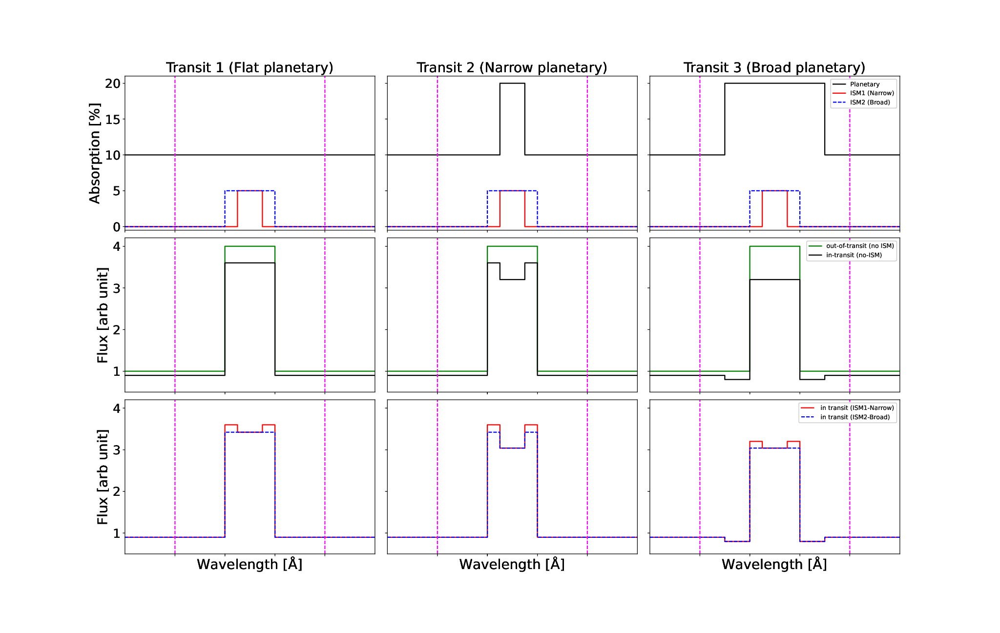
However, this applies to a single wavelength range at infinite spectral resolution and in the ideal case that all involved line profiles have the same shape. Here, we employ the simplified case of rectangular spectral lines (to enable intuitive line integration) to demonstrate that in reality ISM absorption does affect transit depth measurements as a result of different line shapes in combination with a finite spectral resolution. Figure 3 shows a step-by-step construction of three ideal rectangular stellar emission line profiles accounting for different planetary and ISM absorption features, also of rectangular shape. Each of the top panels show three different profiles, one for the planetary absorption (from left to right: constant, narrow, and broad) and two for the ISM absorption (narrow and broad). The middle panels show the stellar emission line profiles before and after planetary absorption, without ISM absorption. The bottom panels show the stellar line profiles following absorption from both planet and ISM. Each panel shows also the integration bin taken into consideration. The top section of Table 1 shows the integrals of the line fluxes in all possible considered cases of ISM and planetary absorption, while the bottom section of Table 1 shows the transit depths obtained from combining the line fluxes. In case of a constant (i.e. not wavelength dependent) planetary absorption, ISM absorption has no influence on the transit depth, but this is not the case when the planetary absorption is wavelength dependent. Furthermore, in case of the narrow planetary absorption feature the deviation from the ISM-free transit depth is greater for the narrow ISM absorption feature, while in case of the broad planetary absorption feature the deviation from the ISM-free transit depth is greater for the broad ISM absorption feature. This demonstrates that ISM absorption can influence transit depth measurements and that this influence depends on the specific shapes of the stellar, ISM, planetary features, spectral resolution, and integration bin in a complicated manner.
| No | Flat | Narrow | Broad | |
|---|---|---|---|---|
| planetary | planetary | planetary | planetary | |
| absorption | absorption | absorption | absorption | |
| No ISM | 6.0 | 5.40 | 5.20 | 4.90 |
| ISM narrow | 5.9 | 5.31 | 5.12 | 4.82 |
| ISM broad | 5.8 | 5.22 | 5.03 | 4.74 |
| - | 0.1000 | 0.1333 | 0.1833 | |
| - | 0.1000 | 0.1322 | 0.1831 | |
| - | 0.1000 | 0.1328 | 0.1828 |
We describe in detail the modeling approach, which aims at reproducing as close as possible the physical and instrumental processes occurring in transit depth measurements obtained from transmission spectroscopy observations covering the Mgii h&k lines. With the parameters described in Section 2, we compute the stellar flux accounting for chromospheric emission, but without ISM absorption () as
| (7) |
where is the stellar photospheric flux and is the Gaussian-shaped Mg ii chromospheric emission. We then obtain the stellar flux during transit () by multiplying the stellar flux to the wavelength-dependent planetary absorption
| (8) |
Then, the in-transit and out-of-transit fluxes including ISM absorption are given by
| (9) |
| (10) |
where is the function simulating the effect of ISM Voigt profiles located at the position of the Mgii h and Mgii k lines.
The fluxes described above are then convolved with the instrument spectral resolution profile to obtain the observed fluxes, that is
| (11) |
| (12) |
| (13) |
and
| (14) |
where IR is the Gaussian shaped instrumental resolution and is the convolution symbol. We further integrate the flux in wavelength bins (see Section 4) and compute the transit depth per integration bin without and with ISM absorption, respectively, as
| (15) |
and
| (16) |
We finally extract the impact of ISM absorption on the transit depth by computing the difference between and (i.e. = -) for a given integration bin as a function of the input parameters. Following Table 1, should be negative. The parameter is a measure of the influence of not considering the impact of Mgii ISM absorption in transit depth measurements covering the Mgii h&k lines. At infinite resolution and at situations not considering the instrument broadening and integration bins the value of would be zero, but when instrument resolution and integration bins comes into play has a non-zero value indicating that this effect is geometrical in nature caused by differences in shape and strength of the chromospheric emission, the planetary absorption, and the interstellar absorption features, in a similar fashion to that of the RLB effect (Deming & Sheppard 2017). To enable a generalisation of the results, we ignore a range of second-order physical phenomena, such as the motion of planetary absorption features during a transit (Snellen et al. 2010, e.g.), the (atmospheric) Rossiter-McLaughlin effect (Borsa et al. 2019, e.g.), center-to-limb variations (Yan et al. 2017, e.g.), stellar spots and flares affecting line emission, and limb darkening.
4 Results

.

We present here the impact of varying the input parameters on to identify the effect of unresolved or unconsidered Mgii ISM absorption in transit depth measurements and transmission spectra. Unless otherwise stated, all results presented below have been obtained considering a Sun-like star (i.e. = 5800 K; = 1 ). Furthermore, in the following when not varying a certain input parameter, we used the default values that are = 100 erg cm-2 s-1, = 12.5, = 3 km s-1, = 0 km s-1, = 30000, an integration bin of 5 Å, and a width of the planetary absorption features of 1.5 Å.
As the transit depth measurement depends on the integration window, our first analysis involved varying the integration bin for different input parameters. Figure 4 illustrates the definition of integration bin considered in this work. The integration bin corresponds to the sum of two equal bins centered on each of the Mgii lines. For example, an integration bin of 2 Å (solid magenta vertical lines in Figure 4) corresponds to two 1 Å wide bins centred around each of the Mgii lines. To avoid discontinuities, when the integration bin becomes large enough that the two bins centred on each line start overlapping (at 7.2 Å bin around each line), the integration bin becomes a single bin centred in the middle of the Mgii lines (e.g. dash-dotted magenta vertical lines in Figure 4).
4.1 Impact of spectral resolution
The bottom panel of Figure 4 shows how varies as a function of integration bin, for the three considered spectral resolution values. We find that ignoring ISM absorption leads to underestimating the transit depth. At high spectral resolution and for small integration bins, || is large, while with increasing integration width || first decreases sharply as a result of considering more stellar flux unaffected by the ISM absorption, and then increases gently until it reaches a maximum, which occurs at a position corresponding to the integration bin that covers exactly the whole of the Mgii planetary absorption feature. Beyond this point, decreases gently towards zero with increasing integration bin. At lower spectral resolution, the behaviour is similar, except for a significant flattening of the variations as a function of integration bin. Figure 4 indicates that the spectral resolution plays a role at small integration bins, while at large integration bins the spectral resolution has no noticeable effect on . With the considered set of parameters, the impact of ignoring ISM absorption at the core of the Mgii h&k lines in transit depth measurements is typically small for integration bins that contain the whole of the ISM absorption features, and does not reach the 0.1% level, that is below the typical uncertainties of NUV transit depth measurements (Fossati et al. 2010; Haswell et al. 2012; Sing et al. 2019; Cubillos et al. 2020, see e.g.).
4.2 Impact of planetary and stellar parameters
We study the impact of the considered Mgii planetary absorption on . We computed considering both 5% and 10% peak absorption at the position of the Mgii k line and, for each of them, three planetary absorption line widths of FWHM equal to 0.75, 1.5, and 3.0 Å. These calculations have been done using the default parameters. Figure 5 (top-left) shows that || increases with increasing planetary Mg ii absorption. We also find that || initially decreases for very small integration bins and then increases with decreasing width of the planetary absorption features. Furthermore, as expected, the position of the second peak of || moves towards larger integration bins with increasing width of the planetary absorption features, demonstrating the tight relation between these two quantities. As mentioned in Section 2.2, our calculations assume that the planetary atmospheric gas responsible for the absorption is optically thin, which is often not the case. Therefore, we show in Figure 6 how varies as a function of integration bin for three different values of the ratio of the Mgii k to Mgii h line strength of the planetary atmospheric absorption, namely values of 2 (i.e. about what given by the values), 1.5, and 1 (i.e. equal line strength). Figure 6 indicates that the impact of line strength ratio is negligible compared to the size of the typical uncertainties of NUV transit depth measurements, and thus that the assumption of optically thin planetary atmospheric gas does not affect the general results. However, Figure 6 also shows that line strength ratio should be considered as a further free parameter for precisely computing .

We further study the impact of stellar parameters on . We compute considering three stars of spectral type K5 ( = 4400 K), G2 ( = 5800 K), and F5 ( = 6500 K) and, for each of them, we consider both 5% and 10% peak planetary absorption at the position of the Mgii k line. The results are shown in Figure 5 (top-right). We find that stellar spectral type has a significant impact on the shape of as a function of the integration bin and in particular is on average larger for later spectral types. This is because the cooler the star the more important the chromospheric emission with respect to the photospheric emission. Therefore, the relative importance of the ISM absorption, which lies on top of the chromospheric emission that is absorbed by the planet, increases with decreasing stellar effective temperature. Furthermore, the top-right panel of Figure 5 indicates that for cooler stars || decreases initially for very small integration bins and then increases with increasing integration bin, which would be against the expectation. However, for cooler stars || behaves as for hotter stars, but the position of the maximum is located at an integration bin that is beyond the shown range and then decreases at larger integration bins, as expected. Again, this stems out of the strong chromospheric emission that overwhelms the photospheric emission for K- and later type stars.
We also compute considering a Sun-like star, three different values of 50, 100, and 200 erg cm-2 s-1, and for each of them both 5% and 10% peak planetary absorption at the position of the Mgii k line. The results are shown in the middle-left panel of Figure 5, which indicates that || sharply decreases initially and then increases with increasing and also that the peak of || moves towards larger integration bins with increasing .
4.3 Impact of ISM parameters
The ISM absorption features have three main components that can affect , namely , the -parameter, and . Employing the spectrographs on-board HST, Redfield & Linsky 2002 measured these three parameters for a large number of stars lying within 100 pc. Therefore, we consider the results of Redfield & Linsky 2002 as a reference for varying the parameters describing the ISM absorption.
We computed setting the Mgii column density at 1011, 3.21012, and 1014 cm-2. For each of them, we further considered both 5% and 10% peak planetary absorption at the position of the Mgii k line. Figure 5 (middle-right) shows that || increases with increasing . Similarly, we varied also the -parameter between 1 and 5 km s-1 obtaining that || increases with increasing (bottom-left panel of Figure 5).
We also looked at the effect of varying keeping all other parameters constant at their default values, for the two considered peak values of the planetary absorption at the position of the Mgii k line (i.e. 5% and 10%). In particular, we varied between 50 and 50 km s-1 in steps of 25 km s-1. Because we model the synthetic chromospheric emission and ISM absorption features as symmetric features, the results obtained considering positive values are almost identical to those obtained considering negative values, where the differences are due to the fact that the photospheric stellar spectrum presents metal absorption lines around the core of the Mgii lines that are not symmetrically placed with respect to the Mgii line cores (e.g. top panel of Figure 4). However, these differences are negligible and we ignore them in the presentation of the results shown in the bottom-right panel of Figure 5. We find that || is larger for smaller values, namely where the ISM absorption features lie closer to the maximum of the stellar emission. For large values and small integration bins, varies significantly as a function of bin size. This is due to the fact that for values of 30–50 km s-1 other photospheric lines begin to play a role, while the ISM absorption features are located close to the minimum of the stellar emission.
4.4 Impact of emission width
As mentioned in Section 2, the width of the chromospheric Mgii stellar emission varies as a function of stellar type and luminosity. Thus we further check whether this plays a role in the shape of as a function of integration bin. To this end, we further derived the width of the Mgii h&k line emission from an HST/STIS observation of the early K-type star Eri obtaining values of 0.394 and 0.431 Å, respectively, which are slightly lower than those we measured for Cen A, which is an early G-type star.
Figure 7 shows how varies as a function of integration bin considering the stellar parameters (Temperature: 4975 K; Radius: 0.83 ) of Eri given by Gaia Collaboration et al. 2018 and the two set of chromospheric line emission widths (i.e. as obtained from the spectra of Cen A and Eri), all other parameters being as the default ones. On average, we find larger || values considering smaller chromospheric line widths, but in general the impact of the stellar emission line width on || is small, particularly when compared to the typical uncertainties of NUV transit depth measurements.

5 Discussion
Figures 9 to 14 show as a function of (ranging between 1010 and 3.21015 cm-2) and (ranging between 50 and 50 km s-1), and for the two peak values of the planetary absorption at the position of the Mgii k line of 5% and 10% we consider in this work. In each plot, we further individually vary spectral resolution (Figure 9), integration bin (Figure 10), FWHM of the planetary absorption (Figure 11), stellar spectral type (Figure 12), value (Figure 13), or -parameter (Figure 14). For all cases and unless specified, we consider a Sun-like star and fix equal to 100 erg cm-2 s-1, the -parameter equal to 3 km s-1, equal to 30000, the FWHM of the planetary absorption features equal to 1.5 Å, and an integration bin equal to 5.0 Å.
The maximum of || shown in these plots is about 0.004, which is comparable to the uncertainties of previous NUV transmission spectroscopy measurements presented by Fossati et al. 2010, Sing et al. 2019, and Cubillos et al. 2020, in the region covered by the Mgii h&k lines (though the integration bins are different in the three works). However, the average value of || is of the order of 0.001 which is smaller than the typical uncertainties of the NUV transmission spectroscopy observations published so far. We remark that the properties of the ISM absorption we considered are realistic, since they are based on results of ISM absorption measurements for stars within 100 pc.
In the following, we present an open-source tool enabling one to estimate on the basis of parameters given by the user and the algorithm described in Section 2 and 3. We also present the value obtained employing this tool for a few systems observed, or soon to be observed, in the NUV.
5.1 Correcting for unresolved Mgii ISM absorption in transit depth measurements
As shown in the previous sections, estimating requires one knowing the shape of the planetary transmission spectrum, of the ISM absorption features, and of the stellar lines. Therefore, it is not possible to accurately evaluate , particularly in the cases when the ISM absorption features and/or the stellar Mgii h&k lines are not well resolved. Estimating requires models of the planetary transmission spectrum and possibly estimates of the ISM absorption and Mgii emission features based mostly on scaling relations. Furthermore, once these ingredients are known, one has to evaluate their impact on considering the complicated interplay among the many parameters involved. To aid in this task, we developed an open-source tool22 2 https://sites.google.com/view/geco-exoplanets/home/software?authuser=0, available both in Python and IDL, enabling one to estimate following the recipes presented above and scaling relations for estimating the Mgii h&k line core emission and ISM absorption that we describe below.
The code requires as input the stellar effective temperature (in K), stellar radius (in ), disk-integrated Mgii h&k line core emission at the distance of 1 AU (i.e. in erg cm-2 s-1), the broad-band (i.e. continuum) NUV transit depth, the peak transit depth at the position of the Mgii k line, the width of the planetary absorption features (in Å), , (in km s-1), the instrumental spectral resolution (in Å), and the size of the integration bin (in Å). Based on the results of Redfield & Linsky 2002, we fix the -parameter equal to 3 km s-1. To run the code, the user has to provide as input at least , the broad-band (i.e. continuum) NUV transit depth, the peak of the transit depth at the position of the Mgii k line, the width of the planetary absorption features, , and the size of the integration bin. If unavailable, the other parameters are derived by the code from assumptions and scaling relations. If not given by the user, the stellar radius is obtained by interpolating on Table 5 of Pecaut & Mamajek 2013. Instead, the code derives the Mgii chromospheric emission on the basis of the value (given by the user as an extra input parameter) and the ISM parameters on the basis of literature results and interstellar reddening (given by the user as an extra input parameter), as described below.
5.1.1 Mg ii h&k line core emission from measurements
The parameter is a measure of the chromospheric emission in the core of the Caii H&K lines and as such, once appropriately calibrated, can be used to estimate the chromospheric emission in the core of the Mgii h&k lines. We employed measurements collected by Sreejith et al. 2020 and Mgii h&k line core emission measurements given by Linsky et al. 2013 to develop scaling relations between the two quantities as a function of stellar spectral type. To this end, we follow the same approach described by Sreejith et al. 2020 and find that and are linearly correlated as
| (17) |
where the and coefficients are listed in Table 2.

| Sp. Type | c1 | c2 |
|---|---|---|
| F, G | 0.87 | 5.73 |
| K | 1.01 | 6.00 |
| M | 1.59 | 6.96 |
If the user does not insert the value in the code, then the code requests the parameter to compute as described above. Also, the code selects the spectral type required to select the parameters to use for the calibration (Table 1) on the basis of and Table 5 of Pecaut & Mamajek 2013.
5.1.2 Deriving Mg ii ISM parameters
If the user does not insert the Mgii ISM parameters, the code assumes to be equal to 0 km s-1 and the -parameter to be equal to 3 km s-1, while is derived from literature results as follows. The Mgii ISM column density is computed employing the Mg ISM abundance and ionisation fraction given by Frisch & Slavin 2003 (their Table 5) as
| (18) |
where (Savage & Mathis 1979)
| (19) |
is the total hydrogen column density (i.e. HHiHii atoms cm-2) as a function of the stellar reddening , which has to be provided by the user.
5.2 Relevance for exoplanet studies
We apply the code described above to a few specific systems that have been observed in the NUV or are soon going to be. The aim is to compare with the observational uncertainties to identify the potential impact of ISM absorption on transit depth measurements and thus on transmission spectra. In particular, we look at WASP-12b (Fossati et al. 2010; Haswell et al. 2012), WASP-121b (Sing et al. 2019), HD209458b (Cubillos et al. 2020), which have been observed with HST, and KELT-9b, which is going to be one of the first targets that is going to be observed by the CUTE SmallSat mission (Fleming et al. 2018).
WASP-12b (Hebb et al. 2009) has been the first exoplanet to be observed at NUV wavelengths (Fossati et al. 2010; Haswell et al. 2012). We estimated the impact of Mgii ISM absorption on the transit depths measured by Fossati et al. 2010 and Haswell et al. 2012 considering the stellar parameters given by GAIA (Gaia Collaboration et al. 2018). Following the discussion of Fossati et al. 2013, we estimated the Mgii chromospheric emission employing a value of 5.1 and the conversion presented in Section 5.1.1. We used the bluest value in the optical transmission spectrum presented by Sing et al. 2016 as the broadband transit depth. The peak transit depth at the position of the Mg ii k line was estimated on the basis of the transit depth measured by Fossati et al. 2010 and considering that the measurement has been obtained using an integration bin of about 20 Å. We further assumed a width of the planetary absorption feature of 1.5 Å, following what obtained by Sing et al. 2019 for WASP-121b. The ISM parameters were derived as described in Section 5.1.2 and employing the reddening inferred from the ISM absorption maps of Amôres & Lépine 2005 and the GAIA distance. For an integration bin of 20 Å corresponding to that of the observations, we find a value of , which is well within the measurement uncertainties (Fossati et al. 2010; Haswell et al. 2012, 0.5%;).
WASP-121b is a transiting hot Jupiter, similar to WASP-12b, with an orbital period of 1.27 days (Evans et al. 2017). Sing et al. 2019 analysed NUV HST/STIS transit observations covering the Mgii h&k lines detecting the presence of both Mg and Fe in the upper planetary atmosphere. We estimated the stellar, chromospheric emission, and ISM absorption parameters as we have done for WASP-12b, while we considered the strength of the planetary absorption observed by Sing et al. 2019. At the resolution of the STIS spectrograph and for the integration bin of 10 Å employed by Sing et al. 2019, we find a value of , which suggests that the measured Mgii transit depth may have been slightly underestimated, though the obtained value is within the 1 observational uncertainties.
HD209458b was the first discovered transiting planet (Charbonneau et al. 2000; Henry et al. 2000) and one of the most well studied planets with several species detected in its atmosphere (Giacobbe et al. 2021, e.g.). Cubillos et al. 2020 reanalysed the NUV HST/STIS transmission spectroscopy observations of HD209458b originally presented by Vidal-Madjar et al. 2013 detecting Fe, but not Mg, in the planetary upper atmosphere, suggesting that the planet hosts Mg-bearing aerosols in the lower atmosphere. We obtained the stellar parameters from GAIA (Gaia Collaboration et al. 2018) and employed a value of 4.97 to infer the Mgii chromospheric emission. We estimated the Mgii ISM column density from the Hi ISM column density measured by Wood et al. 2005 and the scaling relations given in Section5.1.2. As for WASP-12b, we used the bluest value in the optical transmission spectrum presented by Sing et al. 2016 as the broadband transit depth. Because of the Mgii non-detection, we considered peaks of the planetary absorption at the position of the Mgii k line smaller than 5% and a width of 1.5 Å. We find a value of 0.023 for an integration bin of 0.23 Å and of 4.33 for an integration bin of 0.93 Å (Cubillos et al. 2020, see the top and bottom panels of Figure 5 of). For HD209568b, the weaker ISM absorption due to the closer distance to the star leads to positive values indicating that ISM absorption would in principle lead to overestimate the transit depth. However, Cubillos et al. 2020 did not find any planetary absorption signal and thus our results strengthen the non-detection as ISM absorption would not be able to hide the planetary absorption signal in this case.
KELT-9b is an ultra-hot Jupiter orbiting an early A-type star every 1.5 days (Gaudi et al. 2017). As a result of its high atmospheric temperature and bright host star, this is one of the currently most studied planets and a high-priority target for the CUTE SmallSat. We obtained the stellar parameters and estimated the ISM parameters as for WASP-12b. We assumed a broadband transit depth equal to that obtained in the optical (Gaudi et al. 2017) and considered a peak value of the planetary absorption at the position of the Mgii k line of 10%. For an integration bin of 5 Å and at the resolution of HST/STIS and CUTE, we find values of and , respectively, that is significantly smaller than the uncertainties one expects to obtain from the observations (Sreejith et al. 2019, e.g.).
6 Conclusion
We studied and quantified the impact of unresolved or unconsidered Mgii ISM absorption in the core of the Mgii h&k lines on transit depth measurements. We carried out this work employing synthetic spectra, varying a number of stellar, planetary, ISM, instrumental, and analysis parameters. The bias induced by ignoring ISM absorption might lead to overestimate or underestimate transit depths, depending on the specific input parameters. Our parameter study showed that in general || (i.e. the difference in transit depth obtained considering ISM absorption and ignoring it) increases with decreasing stellar temperature, increasing Mgii chromospheric emission, increasing planetary absorption, decreasing planetary absorption width, increasing ISM absorption, and increasing -parameter. || is also maximum when the ISM absorption and chromospheric emission features overlap (i.e. equal to 0 km s-1). We also find that the integration bin considered for computing the transit depth plays a key role in determining the value of , with typically decreasing with increasing integration width.
From all runs we carried out, we found maximum values of the order of 0.005–0.01, though the actual values depend strongly on the involved parameters. The average values we obtain are of the order of 0.0005–0.001, which is smaller than the uncertainties typically obtained with the currently available facilities. As an example, we estimated for WASP-12b, WASP-121b, HD209458b, and KELT-9b, which have been or are soon going to be observed in the NUV. In all cases, we obtained values smaller than the observational uncertainties. However, this may not be the case of observations carried out employing future, larger facilities (e.g. HABEX, LUVOIR) for which the observational uncertainties would be significantly smaller.
Acknowledgements
A.G.S. and L.F. acknowledge financial support from the Austrian Forschungsförderungsgesellschaft FFG projects CONTROL P865968 and CARNIVALS P885348. This project was also partly funded by the Austrian Science Fund (FWF) [J 4596-N]. P.C. acknowledges support and funding by the Austrian Science Fund (FWF) Erwin Schroedinger Fellowship program J4595-N. We thank the anonymous referee for their comments that helped to significantly improve the paper.
Data Availability
The data underlying this article will be shared on reasonable request to the corresponding author.
References
- Amôres & Lépine (2005) Amôres E. B., Lépine J. R. D., 2005, AJ, 130, 659
- Asplund et al. (2009) Asplund M., Grevesse N., Sauval A. J., Scott P., 2009, ARA&A, 47, 481
- Ayres (1979) Ayres T. R., 1979, ApJ, 228, 509
- Borsa et al. (2019) Borsa F., et al., 2019, A&A, 631, A34
- Bourrier et al. (2017) Bourrier V., et al., 2017, A&A, 602, A106
- Bourrier et al. (2018) Bourrier V., et al., 2018, A&A, 620, A147
- Charbonneau et al. (2000) Charbonneau D., Brown T. M., Latham D. W., Mayor M., 2000, ApJ, 529, L45
- Cubillos et al. (2020) Cubillos P. E., Fossati L., Koskinen T., Young M. E., Salz M., France K., Sreejith A. G., Haswell C. A., 2020, AJ, 159, 111
- Debrecht et al. (2018) Debrecht A., Carroll-Nellenback J., Frank A., Fossati L., Blackman E. G., Dobbs-Dixon I., 2018, MNRAS, 478, 2592
- Deming & Sheppard (2017) Deming D., Sheppard K., 2017, ApJ, 841, L3
- Dwivedi et al. (2019) Dwivedi N. K., et al., 2019, MNRAS, 487, 4208
- Ehrenreich et al. (2012) Ehrenreich D., et al., 2012, A&A, 547, A18
- Ehrenreich et al. (2015) Ehrenreich D., et al., 2015, Nature, 522, 459
- Evans et al. (2017) Evans T. M., et al., 2017, Nature, 548, 58
- Fleming et al. (2018) Fleming B. T., et al., 2018, Journal of Astronomical Telescopes, Instruments, and Systems, 4, 014004
- Fossati et al. (2010) Fossati L., et al., 2010, ApJ, 714, L222
- Fossati et al. (2013) Fossati L., Ayres T. R., Haswell C. A., Bohlender D., Kochukhov O., Flöer L., 2013, ApJ, 766, L20
- Fossati et al. (2017) Fossati L., et al., 2017, A&A, 601, A104
- Fossati et al. (2021) Fossati L., Young M. E., Shulyak D., Koskinen T., Huang C., Cubillos P. E., France K., Sreejith A. G., 2021, A&A, 653, A52
- Frisch & Slavin (2003) Frisch P. C., Slavin J. D., 2003, ApJ, 594, 844
- Gaia Collaboration et al. (2018) Gaia Collaboration et al., 2018, A&A, 616, A1
- Gaudi et al. (2017) Gaudi B. S., et al., 2017, Nature, 546, 514
- Giacobbe et al. (2021) Giacobbe P., et al., 2021, Nature, 592, 205
- Green et al. (2012) Green J. C., et al., 2012, ApJ, 744, 60
- Guinan et al. (2016) Guinan E. F., Engle S. G., Durbin A., 2016, ApJ, 821, 81
- Gunár et al. (2021) Gunár S., Koza J., Schwartz P., Heinzel P., Liu W., 2021, ApJS, 255, 16
- Hall (2008) Hall J. C., 2008, Living Reviews in Solar Physics, 5, 2
- Haswell (2010) Haswell C. A., 2010, Transiting Exoplanets
- Haswell et al. (2012) Haswell C. A., et al., 2012, ApJ, 760, 79
- Hebb et al. (2009) Hebb L., et al., 2009, ApJ, 693, 1920
- Henry et al. (2000) Henry G. W., Marcy G. W., Butler R. P., Vogt S. S., 2000, ApJ, 529, L41
- Jin & Mordasini (2018) Jin S., Mordasini C., 2018, ApJ, 853, 163
- Kubyshkina et al. (2018) Kubyshkina D., et al., 2018, A&A, 619, A151
- Kupka et al. (1999) Kupka F., Piskunov N., Ryabchikova T. A., Stempels H. C., Weiss W. W., 1999, A&AS, 138, 119
- Lecavelier Des Etangs (2007) Lecavelier Des Etangs A., 2007, A&A, 461, 1185
- Lecavelier des Etangs et al. (2012) Lecavelier des Etangs A., et al., 2012, A&A, 543, L4
- Linsky et al. (2013) Linsky J. L., France K., Ayres T., 2013, ApJ, 766, 69
- Lopez & Fortney (2013) Lopez E. D., Fortney J. J., 2013, ApJ, 776, 2
- Lothringer et al. (2022) Lothringer J. D., et al., 2022, Nature, 604, 49
- Nichols et al. (2015) Nichols J. D., et al., 2015, ApJ, 803, 9
- Owen & Wu (2017) Owen J. E., Wu Y., 2017, ApJ, 847, 29
- Pecaut & Mamajek (2013) Pecaut M. J., Mamajek E. E., 2013, ApJS, 208, 9
- Piskunov et al. (1995) Piskunov N. E., Kupka F., Ryabchikova T. A., Weiss W. W., Jeffery C. S., 1995, A&AS, 112, 525
- Redfield & Linsky (2002) Redfield S., Linsky J. L., 2002, ApJS, 139, 439
- Ryabchikova et al. (1999) Ryabchikova T. A., Piskunov N. E., Stempels H. C., Kupka F., Weiss W. W., 1999, Physica Scripta Volume T, 83, 162
- Salz et al. (2019) Salz M., Schneider P. C., Fossati L., Czesla S., France K., Schmitt J. H. M. M., 2019, A&A, 623, A57
- Savage & Mathis (1979) Savage B. D., Mathis J. S., 1979, ARA&A, 17, 73
- Shulyak et al. (2004) Shulyak D., Tsymbal V., Ryabchikova T., Stütz C., Weiss W. W., 2004, A&A, 428, 993
- Sing et al. (2016) Sing D. K., et al., 2016, Nature, 529, 59
- Sing et al. (2019) Sing D. K., et al., 2019, AJ, 158, 91
- Snellen et al. (2010) Snellen I. A. G., de Kok R. J., de Mooij E. J. W., Albrecht S., 2010, Nature, 465, 1049
- Sreejith et al. (2019) Sreejith A. G., Fossati L., Fleming B. T., France K., Koskinen T., Egan A., Rüdisser H. T., Steller M., 2019, Journal of Astronomical Telescopes, Instruments, and Systems, 5, 018004
- Sreejith et al. (2020) Sreejith A. G., Fossati L., Youngblood A., France K., Ambily S., 2020, A&A, 644, A67
- Vidal-Madjar et al. (2003) Vidal-Madjar A., Lecavelier des Etangs A., Désert J. M., Ballester G. E., Ferlet R., Hébrard G., Mayor M., 2003, Nature, 422, 143
- Vidal-Madjar et al. (2013) Vidal-Madjar A., et al., 2013, A&A, 560, A54
- Wakeford et al. (2020) Wakeford H. R., et al., 2020, AJ, 159, 204
- Wilson & Vainu Bappu (1957) Wilson O. C., Vainu Bappu M. K., 1957, ApJ, 125, 661
- Wood et al. (2005) Wood B. E., Redfield S., Linsky J. L., Müller H.-R., Zank G. P., 2005, ApJS, 159, 118
- Yan et al. (2017) Yan F., Pallé E., Fosbury R. A. E., Petr-Gotzens M. G., Henning T., 2017, A&A, 603, A73
- Youngblood et al. (2022) Youngblood A., Pineda J. S., Ayres T., France K., Linsky J. L., Wood B. E., Redfield S., Schlieder J. E., 2022, ApJ, 926, 129
Appendix A


