Operator growth in open quantum systems: lessons from the dissipative SYK
Abstract
We study the operator growth in open quantum systems with dephasing dissipation terms, extending the Krylov complexity formalism of Parker:2018yvk. Our results are based on the study of the dissipative -body Sachdev-Ye-Kitaev (SYKq) model, governed by the Markovian dynamics. We introduce a notion of “operator size concentration” which allows a diagrammatic and combinatorial proof of the asymptotic linear behavior of the two sets of Lanczos coefficients ( and ) in the large limit. Our results corroborate with the semi-analytics in finite in the large limit, and the numerical Arnoldi iteration in finite and finite limit. As a result, Krylov complexity exhibits exponential growth following a saturation at a time that grows logarithmically with the inverse dissipation strength. The growth of complexity is suppressed compared to the closed system results, yet it upper bounds the growth of the normalized out-of-time-ordered correlator (OTOC). We provide a plausible explanation of the results from the dual gravitational side.
1 Introduction
A proper understanding of operator growth in dissipative systems is of fundamental interest. This is because dissipative phenomena are ubiquitous in nature and for any practical purposes, it is desirable to understand the effect of the environment on the system itself. One can consider the system plus the environment as a whole system that follows the unitary dynamics Breuer2007. Tracing out the environment leads the system dynamics to non-unitary. However, for the Markovian environment, the system dynamics can be efficiently formulated in terms of Lindbladian evolution Lindblad1976; Gorini. The Lindbladian consists of two parts, a part usually known as the Hermitian Liouvillian which governs the unitary closed system dynamics, and another part which includes the information of the environment. This part is not Hermitian and thus makes the whole evolution non-unitary.
There has been a growing interest to study operator growth in systems whose dynamics are governed by such Lindbladian. Especially it is of utmost interest how the environment affects the chaotic and integrable nature of the system PhysRevLett.61.1899; PhysRevLett.123.254101; Xu:2020wky. Several recent studies have taken promising approaches using different probes, namely, the spectral statistics Li:2021kuv; Garcia-Garcia:2021rle; Matsoukas-Roubeas:2022odk; Kawabata:2022cpr, operator-size distribution Zhang:2022knu; Omanakuttan:2022ikz; pfz, the out-of-time-ordered correlator (OTOC) PhysRevA.103.062214; Schuster:2022bot; Weinstein:2022yce; Syzranov:2017zyp, and Krylov (K-)complexity Parker:2018yvk; Bhattacharya:2022gbz; Liu:2022god.
In this paper, we aim to study the operator growth in the dissipative Sachdev-Ye-Kitaev (SYK) model from the point of view of the K-complexity Parker:2018yvk (for an incomplete list of studies, see Rabinovici:2020ryf; Jian:2020qpp; Barbon:2019wsy; Dymarsky:2019elm; Cao:2020zls; Dymarsky:2021bjq; Caputa:2021sib; Rabinovici:2021qqt; Bhattacharjee:2022vlt; Balasubramanian:2022tpr; Hornedal:2022pkc; Caputa:2021ori; Bhattacharjee:2022ave; Bhattacharjee:2022qjw; Balasubramanian:2022dnj; Rabinovici:2022beu; He:2022ryk; Guo:2022hui and the references therein). The SYK model is a -dimensional quantum mechanical model which consists of fermions where of them are interacting at a time PhysRevLett.70.3339. The model is integrable for and chaotic for . Moreover, the model is exactly solvable, and it is particularly analytically tractable in the large and the large limit Maldacena:2016hyu. In particular, at low temperatures, it shows an emergence of conformal symmetry which allows writing a Schwarzian action Maldacena:2016hyu. This action shares close similarity with the effective action in AdS2 gravity Maldacena:2016upp, for which it received considerable attention from the holographic side Kittu; Cotler:2016fpe. The chaotic nature of this model is well captured by OTOC, satisfying the chaos bound Maldacena:2015waa. Several recent studies have also studied K-complexity in SYK analytically for closed system Parker:2018yvk; Bhattacharjee:2022ave and numerically for closed Jian:2020qpp; Rabinovici:2020ryf and open/dissipative systems Liu:2022god. The numerical results are performed for finite and finite (especially ) Jian:2020qpp; Rabinovici:2020ryf; Liu:2022god, where the Krylov bases have been constructed using the Lanczos algorithm Lanczos1950AnIM. For the dissipative systems, one can implement the algorithms suitable to non-unitary dynamics, namely the Arnoldi iteration Arnoldipaper, which was studied in Bhattacharya:2022gbz. The algorithms are numerical, thus one needs to restrict to a finite number of fermions. However, to see the universal properties of the Lanczos coefficients, especially its asymptotic growth in the presence of the environment, analytical studies are highly desirable. Here we report some analytical results in the large and the large limit for the dissipative SYK which has not been reported before.
The dissipative model we choose is proposed by Kulkarni, Numasawa and Ryu Kulkarni:2021xsx (see Sa:2021tdr for a similar model). Recently, it has been shown that the model is dual to a non-Hermitian two-site SYK model at low temperature, connected by a Keldysh wormhole Garcia-Garcia:2022adg. It is closely analogous to a Maldacena-Qi Maldacena:2018lmt coupled SYK model, albeit with some significant differences. To establish our results, we take several different approaches. First, we give a diagrammatic and combinatorial proof of our claim Eq. (22) and Eq. (23) for the SYK model. The proof relies on the expansion, introducing the notion of “operator size concentration”. Then we give an analytical check by generalizing the method of moments viswanath1994recursion. Previously, a specific version of this method was applied to closed systems Parker:2018yvk; Bhattacharjee:2022ave. We extract the analytical form of two sets of Lanczos coefficients, which correspond to the primary diagonal and primary off-diagonal elements of the Lindbladian matrix written in Krylov basis Bhattacharya:2022gbz. We find that only the diagonal elements of the Lindbladian are sensitive to dissipation. We confirm our analytical results by semi-analytics in finite and large limit, and by directly implementing the numerical Arnoldi iteration in finite and finite limit. We emphasize that these three different approaches have their own advantages and disadvantages, in lieu of capturing the K-complexity behavior, for different types of systems. It is demonstrated that the large limit of the dissipative SYK model is a unique scenario where these approaches are equally viable.
The consistencies of all the results allow us to conjecture an operator growth hypothesis for the open systems, given by Eq. (59). The analytical expressions of and are then used to derive analytical expressions for the Krylov basis wavefunctions, Krylov complexity, and Krylov variance. These expressions correspond to a special sub-class of the dissipative SYK model, where the dissipation strength is quadratically related to the random coupling . For weak dissipation, this model is a good approximation to the one considered in the rest of the manuscript. As a result, the Krylov complexity exhibits suppressed growth and saturation compared to the exponential growth for the closed systems. We identify the saturation timescale which grows logarithmically to the inverse of the dissipation strength. Although our results are based on the large analysis of the SYK model, we believe the claim of Eq. (59) to hold for any generic open quantum systems. In fact, some analysis on spin systems Bhattacharya:2022gbz; Liu:2022god supports our claim. Based on the above observation, we argue the growth of K-complexity must upper bounds the growth of normalized out-of-time-ordered (OTOC), which might generalize the chaos bound Maldacena:2015waa in open systems. Finally, we speculate a holographic interpretation of our results from the dual gravity side.
The manuscript is structured as follows. In section 2 we review a few recently explored approaches to the K-complexity in open systems. In section 3, we review the dissipative SYK model which will be our main playground. It was introduced in Kulkarni:2021xsx, and more details can be found on Garcia-Garcia:2022adg; Kawabata:2022osw. In section 4, we derive the main analytical results in the large limit. Section 5 presents numerical evidence that these results still hold as an excellent approximation away from large . In 6 we derive the consequences in terms of the main results in terms of K-complexity growth and discuss implications on scrambling. We also give a heuristic explanation of our results from the gravitational side. Finally, section 7 concludes the discussion with some open questions.
2 Krylov complexity in open systems: general approaches
The Krylov (K-)complexity of operators is mostly studied in closed Hamiltonian systems. Extending it to open systems is not straightforward at all, and so far there is no consensus on how one should proceed in general. Here, we restrict our attention to a restricted class of open dynamics that are described by a Lindblad master equation which admits the infinite temperature (maximally mixed) state as a stationary state and focus on the dynamics of operators in this ensemble. Even then, a few approaches are possible (and some have been explored), as we review in this section.
To set the common stage, let us recall the Lindblad equation in its general form Lindblad1976; Gorini:
| (1) |
Here and are the Hamiltonian and the density matrix of the system, and ’s as the jump operators. As mentioned above, we shall assume that
| (2) |
where represents the infinite-temperature state. In this stationary state, it is reasonable to consider the operator dynamics, governed by
| (3) |
where the Heisenberg-picture Lindbladian is given by Bhattacharya:2022gbz
| (4) |
Here, we view as a superoperator acting on the space of operators (the minus sign has to be taken when both and are fermionic operators Liu:2022god). It is written as a sum of a unitary Liouvillian and a dissipation contribution . The space of operators is also endowed with the inner product
| (5) |
Then, the autocorrelation function of an operator can be defined similarly as in the closed-system context:
| (6) |
Without loss of generality, we shall assume that has unit norm: .
2.1 Using the closed Krylov basis
Ref. Li:2021kuv proposed a simple way to extend the notion of K-complexity to the above open setting: we take the Krylov basis generated by the repeated action of the closed-system Liouvillian . Recall that this is an orthonormal basis that spans the Krylov subspaces:
Assuming that the open-system operator dynamics remain in such a Krylov subspace, one can define its K-complexity in exactly the same way. Now, on this basis the full Lindbladian is represented as a general matrix: while becomes tridiagonal, enjoys no special property in general. Nevertheless, the authors of Li:2021kuv put forward conjectures on the matrix elements motivated by numerical study, which we shall discuss below.
2.2 Arnoldi iteration
An alternative method, explored in Ref. Bhattacharya:2022gbz, considers another orthonormal basis , which corresponds to the Krylov subspaces generated by the full open-system Lindbladian:
This basis, as well as the representation of the Lindbladian in it, can be generated by the Arnoldi iteration that we recall now.
We start with an initial normalized vector . For , we construct
| (7) |
Then, for to , we perform the following iterations:
| (8) |
(Stop if .) Otherwise define as
| (9) |
As a result, the Lindbladian is transformed into an upper Hessenberg form in the Krylov basis (sometimes called Arnoldi basis):
| (10) |
where . When is a Hermitian superoperator, the Arnoldi iteration reduces to the Lanczos algorithm, and the above matrix becomes real symmetric and tridiagonal. However, for a general Lindbladian, these properties are not guaranteed. Thus, while the basis allows to define a version of K-complexity, the Lindbladian is still relatively involved.
2.3 The moment method
A distinct approach is to generalize the “moment method” viswanath1994recursion, which was previously studied in closed SYK Parker:2018yvk, and its higher-order corrections Bhattacharjee:2022ave. Rather than constructing a basis, this method focuses on the auto-correlation function, or its derivatives around , known as the moments:
| (11) |
Now, assuming that the superoperator generating the dynamics is Hermitian, the Lanczos coefficients and the moments are related by a nonlinear transform. In terms of the Lanczos coefficients, the moments, encoded in the Green function, can be obtained as a continued fraction expansion viswanath1994recursion; Parker:2018yvk:
| (12) |
From the moments, the Lanczos coefficients can be calculated by a recursive algorithm viswanath1994recursion:
| (13) |
Note that the above relations are a bit more general than those used in Parker:2018yvk, which are valid for the case where the odd moments vanish (this is the case for closed systems and a Hermitian operator , for example). Formally, we can apply the algorithm (13) to the moments of an open-system autocorrelation function, ignoring the above-mentioned assumption. Generically — that is, barring the occurrence of division-by-zero errors — we are guaranteed to obtain two sequences of complex numbers, . However, it should be emphasized that they are not the output of a Lanczos algorithm. In fact, the moment method generates a non-orthonormal basis of the Krylov subspaces, in which is represented as a symmetric tridiagonal matrix
| (14) |
Thus, although we simplified the matrix representation of , it becomes problematic to define the notion of K-complexity using the non-orthonormal basis, which can be in practice quite singular (with respect to the inner product).
To conclude, we reviewed three different attempts to extend the K-complexity to an open-system context. None of them is entirely satisfactory; each of them solves certain problems by making others worse. There seems to be a list of “wishes” that cannot be simultaneously fulfilled in general. The main point of this paper is to show that all wishes can come true in certain systems.
3 The dissipative SYK
In this section, we review and introduce a concrete system, which is a dissipative version of the Sachdev-Ye-Kitaev (SYK) model PhysRevLett.70.3339; Kittu. The SYK model is a -dimensional quantum mechanical model which consists of fermions where of them are interacting at a time. The SYKq Hamiltonian is given by PhysRevLett.70.3339
| (15) |
where ’s are Majorana fermions satisfying , and are random couplings, drawn from some Gaussian ensemble with zero mean and variance . The constant is a dimensionful parameter and sets the energy scale of the Hamiltonian. We will be particularly interested in the limit where we send , and then . In that limit, the model is quantum chaotic yet enjoys a high degree of analytical tractability; numerical studies are required more or less away from this limit. When is large, it is convenient to define a rescaled coupling constant:
| (16) |
To introduce openness, we consider the following jump operators Kulkarni:2021xsx
| (17) |
where is the dissipation strength or that of the system-environment coupling. The dissipation operators are fermionic and Hermitian. The Hermiticity ensures that the infinite-temperature density matrix Kulkarni:2021xsx; Sa:2021tdr; Garcia-Garcia:2022adg is a stationary state. It will be useful to note that, the action of the dissipative part of the Lindbladian is very simple on “Majorana string” operators. For any and , we have
| (18) |
See Appendix A for the derivation. In other words, the effect of the dissipation is to annihilate a Majorana string with a rate proportional to its size and to (recall that the operator evolution is generated by ). Therefore, and have competing effects as the latter makes the operator size grow. In the large limit, we rescale as well, so that
| (19) |
is of order unity Kulkarni:2021xsx.
Often, the dynamics of the operators (as well as of the density matrix) is seen as taking place in the double Hilbert space through the lens of Choi-Jamiolkowski (CJ) isomorphism CHOI1975285; JAMIOLKOWSKI1972275. In this regard, the operator dynamics is generated by the non-Hermitian Hamiltonian Garcia-Garcia:2022adg:
| (20) |
This can be understood as two SYK (with relative phase between them) interacting with the coupling . The state , which is the image of under the CJ-isomorphism, is the ground state of and well as . Note that this is slightly different than Ref. Maldacena:2018lmt, where the Hamiltonian is Hermitian (the imaginary factor is absent in the first two terms). Hence, the dissipative dynamics are equivalent to non-Hermitian dynamics governed by the above Hamiltonian.
4 Large exact result
We are in a position to state the main result of this work: for the dissipative SYK in the large limit with , the three approaches in Section 2 exactly coincide, in the sense that:
- 1.
The closed-system Krylov basis is identical to the open-system one .
- 2.
The Arnoldi iteration yields a symmetric tridiagonal matrix, whose matrix elements are equal to the Lanczos coefficients obtained by the moment method. In particular, we have
(21)
Furthermore, these coefficients are exactly calculated:
| (22) | ||||
| (23) |
Here, the results on are identical to the closed-system one obtained in Parker:2018yvk, which is expected from 1 above. The result on is new and shows that the diagonal elements are imaginary, and grow linearly with with a slope set by the dissipation strength Liu:2022god.
In the rest of this section, we first present a direct derivation of the above results. Then, a nontrivial check of the Lanczos coefficients formulae (22) and (23) via the moment method will be exposed. Finally, numerical results away from the ideal limit will be discussed.
4.1 Operator size concentration
It turns out that the above statements are all corollaries of the following “operator size concentration” property of the Krylov basis elements of the closed SYK model in the large limit: the -th basis operator is a linear combination of Majorana strings of the same size
| (24) |
where
| (25) |
Here is the size and is the generation, according to the nomenclature of Ref. Roberts:2018mnp. Indeed, recall (18) that Majorana strings of size are degenerate eigen-operators of the dissipative part of Lindbladian, with eigenvalue . Thus, (24) implies
| (26) |
where is defined through (19). This, combined with the known action of , implies the statements above as well as (22) and (23) immediately.
It remains to prove operator size concentration (24), which concerns the closed SYK model in the large limit. It is known Roberts:2018mnp; Parker:2018yvk that one can study the operator dynamics and implement the Lanczos algorithm directly in the large limit using “open” melon diagrams. Our proof will rely on this combinatorial approach, which we briefly review. For simplicity we set below.
Let us iteratively apply to and describe graphically the operators generated. It will be convenient to decompose the Liouvillian as Caputa:2021sib
| (27) |
where are the operator-size increasing (decreasing, respectively) contribution to . In other words, is defined such that for two Majorana strings of sizes and ,
| (28) |
is then defined as the Hermitian conjugate of . By applying instead of , we can focus on the new operators generated at each step.
At the first step,
| (29) |
Here, we first represent , which is a -body operator generated from the , by the half of a melon diagram as in Roberts:2018mnp. Since is large, we omit all (grey) propagators but two representatives, and also the tip of the melon. Hence the diagram simplifies to a simple arc.
With this in mind, the next few operators generated will be the following:
| (30) | ||||
| (31) | ||||
| (32) |
and so on. Every time, the acts on one of the Majorana’s inside an arc, and transforms it into Majorana’s represented by a new arc, which we view as a “child” of the former. We can equivalently view the operators appearing in as rooted and unmarked trees with vertices (a vertex = an arc). We remark that equations (30) and (32) are operator identities that are valid before averaging over the disordered couplings , modulo terms that will have negligible contributions to any disordered-averaged observables in the large limit. Each arc involves a dangling disorder line. The subleading terms are neglected by considering only open melon diagrams. The observables can be constructed by closing the open melon diagrams, that is, taking the inner product with another operator and averaging over disorder.
So far, we have been elusive about the prefactors. A neat way to keep track of them is to order the arcs in the diagrams, such that a vertex comes always before its children. For example, the diagram with prefactor above can be ordered in three ways:
In other words, the amplitude of an unmarked diagram in is given by the ways it can be built by adding one arc at a time. Note that the terms of the right-hand side are the same operator; the different orderings enumerate its amplitude (multiplicity) in . As a consequence,
| (33) |
We now come to the essential claim of this section. For any , we have
| (34) |
This identity can be proved diagrammatically. By (33) and the definition of , the left-hand side is a sum of ordered diagrams of arcs with one childless arc marked. For example,
| (35) |
In the second line, the marked childless arc is represented by a red dashed line. One should view it as being removed by the action of .
Now, to prove (34), we shall show that the removal of the marked arc gives rise to an -to-one correspondence between the ensemble of marked and ordered diagrams with arcs, and that of ordered diagrams with arcs. To do this, consider a marked and ordered diagram of arcs, say, . Removing the marked arc gives rise to the following ordered diagram with arcs:
This removal map is not one-to-one, since we lost information about the marked arc, namely, its parent’s index , and its order (since it must come later than its parent). In the above example, in the example. It is not hard to see that the datum of
| (36) |
allows to reconstruct uniquely the marked ordered diagram with arcs from any ordered diagram of arcs. For example,
Observe that removing the marked arc on the right-hand side gives back the diagram on the left-hand side. Since there are
such tuples satisfying (36), the removal map is a -to-one correspondence. This concludes the combinatorial proof of (34).
The key consequence of (34) is that, the Krylov basis generated by and is essentially , up to normalization:
| (37) |
To see this, we first notice that is an orthogonal set, since is a linear combination of Majorana strings of length , and Majorana strings of distinct lengths are orthogonal under the inner product (5). Moreover, by (27) and (34), for ,
| (38) |
The edge cases can be taken care of by explicit calculation:
| (39) |
Therefore, the Liouvillian is represented as a tridiagonal matrix in the basis . Combined with its orthogonality, we conclude that it must be identical to the Krylov basis up to normalization, (37). In fact, (38) implies that the Lanczos coefficients for , as announced in (23) (recall that we set ).** * The square-root comes from the appropriate normalization of , to get . The way to proceed with this is to consider the norm, , which gives the normalization squared. Thus, we have provided an independent, diagrammatic derivation of this nontrivial result (the derivation in Parker:2018yvk relied on the moment method and knowledge about tangent numbers, see also below).
Eq. (37) implies operator size concentration (24) immediately: since is by construction a linear combination of Majorana strings of length , the same is true for the -th Krylov basis element of the large SYK model. This concludes the derivation of the main results announced at the beginning of the section.
4.2 Consequence on moments
A consequence of the main results is that the Lanczos coefficients (22) and (23) are related to the autocorrelation function of the dissipative SYK in the large limit. The latter has been computed explicitly by solving a Schwinger-Dyson equation Kulkarni:2021xsx:** * We remark that the large expansion above is valid for , where is such that , or , for large . Beyond that time scale, the expansion (40) breaks down, and one would need a different approximation Kawabata:2022osw.
| (40) | ||||
| (41) |
where we recall that , and the other variables are given by
| (42) |
In the closed-system case , we recover the known result Maldacena:2016hyu, and the associated moments are essentially the tangent numbers, and the Green function is known to have a continued fraction expansion given by the ’s Parker:2018yvk. When , the moments are considerably more involved. Setting without loss of generality, the moments have the large expansion
| (43) |
and is a polynomial of . For example, ,
| (44) | ||||
| (45) | ||||
| (46) | ||||
| (47) | ||||
| (48) | ||||
| (49) | ||||
| (50) |
and so on. The coefficients appear to coincide with the so-called triangle “”, see A101280 and references therein for further mathematical facts about it. Our main result then implies the following continued fraction formula
| (51) |
One may check this formula order by order in . We are not aware of an independent “elementary” proof. See however discussion around Eq. (77) below.
5 Finite numerics
In this section, we turn to examine how the simple “ideal” scenario established above at the limit is affected at finite .
5.1 Large : operator size distribution
Our main results at the large limit rely on the operator size concentration property of the closed-system Krylov basis. A natural way to anticipate how these results survive at finite is to examine the operator size distribution Roberts:2018mnp; Qi:2018bje. This can still be done in the large limit, by extending the diagrammatic approach to large operators Roberts:2018mnp; Parker:2018yvk described in the previous section to an arbitrary value of : a finite imposes that every arc can have at most (direct) children. Coding this in a computer, we may generate all the large operators up to a certain size, which allows us to implement the Lanczos algorithm in the large limit and construct explicitly the Krylov basis operators, up to a certain value of . (As the number of operators increases exponentially in , we are limited to ; fortunately, this is enough to observe the asymptotic behaviors.)
We then measure the operator size distribution of the Krylov basis operators . In a finite size system, this is defined as follows Roberts:2018mnp: writing as a sum of Majorana strings
| (52) |
the size distribution is then given by
| (53) |
In the large representation, an operator is a sum of diagrams, each representing a sum of Majorana strings with definite size , related to the number of arcs as . The weights depends on the random coupling coefficients . Yet, one can show that each diagram after disorder averaging and summing over fermion flavors, each diagram gives the same weight. Hence, the size distribution can be readily measured at large . Using the size distribution, we can obtain readily the average operator size as well as higher moments.

In Fig. 1 (a), we plot the results for . We observe that the operator size concentration property holds exactly if and only if : only the first five Krylov basis operators are a sum of Majorana’s of a definite size . For larger , the exact operator size concentration is indeed only a property of the large limit.** * We have checked a few other values of and observed that the property always breaks down at . Nevertheless, the distribution of operator size is highly peaked at , which is the maximal operator size present in . The weight of operator sizes decays exponentially fast in , see the inset of Fig. 1 (a). As a result, the mean operator size grows linearly in . Its standard deviation also grows linearly with , yet much more slowly than the mean value. Our numerics indicates the standard deviation-mean ratio tends to be a small constant:
| (54) |
for SYK. Data for other values of suggest that the constant decays as .
In summary, we provided significant evidence indicating that operator size concentration is an excellent approximation in the SYK model for any values of . We may further rationalize this optimism by observing that the operator size concentration holds exactly for (since only Majorana strings of length are generated) as well as for ; hence, it cannot be too wrong at intermediate values of .
5.2 Large : Arnoldi iteration
As a consequence of operator size concentration, we expect that the Arnoldi iteration should result in a matrix close to the “ideal scenario” Bhattacharya:2022gbz; Liu:2022god. That is, to a good approximation,
- 1.
should be a symmetric tridiagonal matrix,
- 2.
its diagonal elements are imaginary and grow linearly in with a pre-factor proportional to :
(55) Here is some -independent proportionality constant.
- 3.
its primary off-diagonal elements grow linearly in :
(56) where is independent of .
This is indeed what we found from our large numerics. In Fig. 1(b) we plot the magnitude of the matrix elements obtained from the Arnoldi iteration. As expected, the largest matrix elements are on the diagonal and primary off-diagonals; the other nonzero elements, that is, for , are about two orders of magnitudes smaller (both the dissipation rate and the unitary coupling constant is of order one, ).
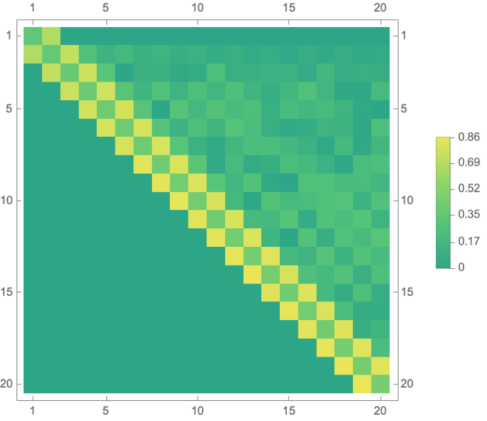
Next, let us examine more quantitatively how close the matrix is to the “ideal scenario”. In Fig. 2 (a), we plot the primary off-diagonal elements (which are real), the imaginary part of the diagonal elements (they turn out purely imaginary), and also an “error” defined as
| (57) |
By definition, the error vanishes if and only if is symmetric. We observe almost perfect linear growth in for both and . The growth rate of is proportional to the dissipation rate while that of is almost independent of it (as long as ). For the values of accessible to us, the error is much smaller for order-unity dissipation . We also observe a rather fast growth of as increases, and cannot rule out the possibility that the matrix deviates significantly from the ideal scenario for sufficiently large. However, for weaker dissipation, the errors appear to be well described by , with a proportionality constant of order . Thus, the matrix should be close to the ideal scenario for . As we shall see below, the operator dynamics will be confined in the region under the ideal scenario, so the deviation from the ideal scenario at larger is irrelevant.
To conclude, the large numerics confirms that operator size concentration is a good approximation at finite , and as a consequence, the Arnoldi iteration results in a matrix close to the “ideal scenario”: symmetric and tridiagonal, with diagonals and primary off-diagonals .
5.3 Arnoldi iteration at finite
We now consider Arnoldi iteration for single realizations of the SYK model at finite , up to , starting from the (normalized) initial operator . A sample of the resulting matrix is plotted in Fig. 2 (b). It is still close to the ideal scenario, modulo the saturation effect induced by the finite system size (see below). The diagonal elements are imaginary and grow linearly with up to the finite size saturation. The growth rate compares well with the prediction (see also Fig. 3(a)):
| (58) |
In other words, in Eq. (55). To obtain (58), we assume that operator size distribution is still a good approximation. Hence, we have , and the operator size distribution of is concentrated at . Then (58) follows from recalling how the dissipative Lindbladian acts on Majorana strings (18). The primary off-diagonals are also not exactly equal, , see Fig. 3 (b), yet the relative difference is small. The magnitudes of the other off-diagonal elements are also small compared to diagonal and primary off-diagonal elements which are manifested in Fig. 2 (b).
Finally, in Fig. 3 (c-d), we exhibit the system size () dependence of the diagonal elements. In Fig. 3 (c), we see a saturation plateau after an initial linear growth for . The saturation value increases linearly with , see Fig. 3 (d). The finite size saturation happens since the Majorana string lengths are upper bounded by , by (18). A similar behavior applies to the primary off-diagonal entries, as in the closed case.
6 Operator growth and Krylov complexity
In the preceding sections, we showed that — exactly at the large and large limit, to a good approximation beyond — the dissipative SYK model displays operator size concentration. As a result, the three approaches of Section 2 coincide, and the Lindbladian acts on the Krylov basis, as a symmetric tridiagonal matrix whose diagonal and primary off-diagonal elements have the following asymptotic growth:
| (59) |
This is also referred to as the “ideal scenario”. The coefficient is the same as in the closed system, whereas depends on how the size of the Krylov basis operator grows with . It may be a bit hasty to discuss how general it is. Even if we restrict to situations where the ideal scenario entails operator size concentration, it is in general unknown how the latter is respected in models away from large ; however, there is numerical evidence indicating that the ideal scenario remains a good approximation in quantum spin chains Bhattacharya:2022gbz; Liu:2022god. We leave a detailed study to the future.
Nevertheless, we can readily examine the consequence of the ideal scenario on the K-complexity growth. For this, we expand the operator on the closed-system Krylov basis:
| (60) |
Note that the norm of the operator is not conserved Liu:2022god: . Thus, we shall define the K-complexity as the average position of the normalized wavefunction:
| (61) |
Under the ideal scenario, the amplitudes satisfy the following differential equation
| (62) |
where and satisfy (59), and initially, the wavefunction is localized at the origin:
6.1 General argument
To understand the asymptotic quantitative behavior in a simple way, we can make the Ansatz that depends on smoothly, and approximate (62) by a PDE:
| (63) |
This equation has a stationary () solution:
| (64) |
It has an exponential tail of width , which is inverse proportional to the dissipation strength , and proportional to the K-complexity growth rate in the closed system . The continuum approach here is quantitatively correct if , i.e., in the weak dissipation regime. In this regime, the dissipation term is negligible for . Now, initially, the wavefunction is localized at origin, so it will evolve as in the case: it is known Parker:2018yvk that it will spread exponentially fast, and its average position . This is true until the wavefunction reaches , where the dissipation term can no longer be neglected. In fact, it suppresses any further growth of the K-complexity, and the wavefunction converges to the stationary solution.** * To be precise, this is true modulo the global normalization, which decays exponentially in the stationary regime; the decay rate depends on details at small. But at large, the spatial profile is still given by (64).
We have thus argued that, under the ideal scenario and in the weak dissipation regime, the exponential growth of the K-complexity saturates at :
| (65) |
Here we also identified the saturation time scale, which diverges as a log of the inverse dissipation strength as — a behavior reminiscent of the scrambling time with respect to a finite system. At strong dissipation, and , the exponential growth regime of disappears.
It is interesting to note that, the “localization” of the operator wavefunction in the region on the Krylov chain protects itself against any deviation from the ideal scenario, provided that happens only at ; We have seen in Section 5.2 that this is indeed the case for the dissipative SYK at finite . It is reasonable to expect this to be general, as the deviation from the ideal scenario necessitates dissipation. Therefore, we believe the K-complexity saturation to be a robust phenomenon in similar situations.
6.2 Exact solution
The above argument, although heuristic, is applicable to any and with the asymptotics (59). Here, we check the conclusion with an exact solvable set of coefficients:
| (66) |
This is precisely the recursion coefficients of the Meixner polynomials used in Ref. Parker:2018yvk (Appendix D, Eq. (D10), upon identifying ; in that work, only was useful). These Lanczos coefficients have the asymptotic behavior (59), with
| (67) |
Varying , we have obtained any relative dissipation strength, (meanwhile does not affect the asymptotic growth rates, but only the offsets).
Following closely ibid. (Eq D11 and D9), it is straightforward to show that
| (68) |
Here is the Pochhammer symbol. Since we will use the normalized wavefunction to define the K-complexity, the first line of (68) (an independent pre-factor) can be ignored. In Fig. 4 (a), we plotted a few wavefunction snapshots from the above exact solution for . We see qualitatively that time evolution is indeed described by the above general argument. Curiously, the coefficients (66) have the same structure of , after identifying the coefficients Balasubramanian:2022tpr and the highest weight state. Hence, the amplitude (68) is fixed by the symmetry, which possibly controls the complexity growth Hornedal:2022pkc. As we see, in our case, the structure is preserved, yet the complexity is suppressed. The suppression entirely comes due to the imaginary part of the coefficients .** * We thank Pawel Caputa for pointing this out.
We can make further quantitative comparisons, focusing on the tail of the wave function. It is not hard to see that at , the wavefunction has the following stationary -dependence for :
| (69) |
We find an exponential decay.** * The power-law correction comes from , after using the asymptotics as . At small (weak dissipation), its inverse width
agrees with the prediction of (64) applied to (67), which gives also . A similar analysis at finite gives
| (70) |
where
| (71) |
The saturation time is given by equating the two terms; we thus find which agrees with (65) at small .
The exact solution above allows us to compute the K-complexity analytically. Indeed, denoting
| (72) |
it is not hard to see from (68) that
| (73) |
See Fig. 4 (b) for a plot. Expanding this around (weak dissipation) at fixed gives
| (74) |
where we recover the exponential growth (with ) in the closed system, as well as the first correction due to dissipation. Now, the latter will dominate at , rendering this expansion useless. Meanwhile, expanding around at fixed , we see that the K-complexity goes to a constant:
| (75) |
It is proportional to at small , and the proportionality constant is controlled by . Hence, the exact calculation confirms the conclusions (65) of the general argument.
Similarly, we can compute the normalized variance Caputa:2021ori; Bhattacharjee:2022ave (note that we define it again using the normalized wavefunction):
| (76) |
It behaves as in the growth regime and saturates at in the late time regime. In both cases, the position fluctuation is comparable to its average .
It is interesting to remark that the Lanczos coefficient (22),(23) of the large SYK corresponds exactly — up to subleading terms in a expansion — to the exact solvable ones (23) upon identifying
| (77) |
As such, our results above apply to the large SYK; in particular, we may recover (40) and (51). The K-complexity in this model is , as most of the wave function is localized at the origin.
6.3 Bound on chaos
We now come back to discussing a general consequence of the saturated K-complexity growth (65). Now, under the ideal scenario, the K-complexity is computed with respect to the closed-system Krylov basis (which is also approximately the basis generated by the Arnoldi iteration). Thus, the argument leading to the bound on chaos in Ref. Parker:2018yvk still applies and entails that the exponential growth of the normalized out-of-time-order correlator (OTOC) must saturate. More precisely and concretely, in the dissipative SYK model, we expect (and have proven at large ) that there exists a -independent constant such that
| (78) |
where is given by (65), with and calculable from the model parameters, and is the norm of the evolved operator. In particular, in the presence of any dissipation, however small it is, the OTOC at the left-hand side cannot grow indefinitely even in the limit. In particular, there is no nonzero critical value of below which the OTOC is in a “chaotic” phase, in contrast to the models studied recently Weinstein:2022yce; Zhang:2022knu. Indeed, the dissipation term in our case has a more severe effect on the terms in with large size (long Majorana strings), which dominate the OTOC. They are simply eliminated (with a rate proportional to the length); meanwhile, in the models of op. cit., the dissipation reduces their sizes without eliminating them altogether.
6.4 Holographic interpretation
Finally, we speculate some heuristic explanations of our results from the dual gravity picture. As argued in Garcia-Garcia:2022adg, the SYK model with the jump operators given by (17) is dual to a Keldysh wormhole. The gravitational geometry of such a wormhole is far from clear. The configuration is valid in real-time and is fundamentally different from the traversable Maldacena:2018lmt or Euclidean wormhole Garcia-Garcia:2020ttf. However, we can still take inspiration from the bulk picture of the growth of operator size Susskind:2018tei; Susskind:2020gnl. The scrambling time in the dissipative SYK appears to be smaller than in the non-dissipative SYK. Increasing the coupling decreases the scrambling time, encountering a possible competition between the scrambling and decoherence Xu:2020wky. In the dual picture, we might think that the particle falling on one side can be reached on the other side due to the coupling like Eq. (20). However, there is still a finite decay rate even at zero dissipation Kulkarni:2021xsx; Garcia-Garcia:2022adg, which is possibly related to the length of the wormhole. The dissipation effectively increases the coupling between the two sides of the wormhole, thus signaling a quicker scrambling. It will be interesting to understand this in a much broader sense, especially computing the complexity in the Jackiw-Teitelboim (JT) gravity Jian:2020qpp. We leave a detailed discussion in future studies.
7 Conclusion
In this paper, we aim to extend the universal operator growth hypothesis in open quantum systems. Our model of study is the dissipative -body SYK model where the interactions with the environment are modeled by the Lindbladian construction. One of the particular motivations is the large limit, where the quantities of interest can be computed analytically. In particular, the “operator size concentration” allows a simple proof to extract two sets of Lanczos coefficients, which can also be exactly computed from the moment method. Out of two sets, only one of the sets is sensitive to dissipation while the other keeps track of the chaotic nature of the Hamiltonian. The asymptotic growth of both sets of coefficients is linear, which can be considered a generalized operator growth hypothesis in the dissipative systems. This result is consistent with the semi-analytics in by solving the Schwinger-Dyson equations and explicit numerical implementation of Arnoldi iteration. The dissipative nature of the environment suppresses the complexity compared to its exponential growth in a closed system. This result corroborates the finds of SYK for finite (thus finite ) and spinless fermionic systems Liu:2022god. We believe that the exponential growth and the consecutive saturation at “scrambling time” is a universal feature to hold any dissipative systems. Finally, we argue some holographic interpretation of the complexity growth of the dissipative SYK, known to be dual to the Keldysh wormhole Garcia-Garcia:2022adg.
While the asymptotic growth of s has been known for integrable systems, it is an open question to ask about the asymptotic growth of the s in generic integrable systems. Some relevant studies have been performed in Bhattacharya:2022gbz, and the growth seems to be not affected due to the integrability of the system. We believe a careful study is required. It will also be worth implementing the numerical bi-Lanczos algorithm gruning, where the “bra” and “ket” vectors in the doubled Hilbert space will evolve differently. The Lindbladian in this bi-orthonormal basis is expected to reproduce the analytical results in the large and large limit. Finally, it is also exciting to see the growth of the complexity with random jump operators Sa:2021tdr, and especially for the dissipative dynamics of complex fermions, where the latter might be equivalent to two non-Hermitian SYK Garcia-Garcia:2022rtg; Cai:2022onu. This might provide a general perspective to establish a “universal” conclusion of our results. A larger and wider motivation is to understand the chaos bound Maldacena:2015waa in dissipative systems, provided it is well-defined in such a scenario. We hope to return to some of these questions in future works.
8 Acknowledgements
X.C. thanks Thomas Scaffidi and Zihao Qi for useful discussions, in particular for pointing out Ref. Liu:2022god. P.N. thanks Pawel Caputa, Tokiro Numasawa, and Shinsei Ryu for the fruitful discussions. P.N. would like to thank the organizers of Kavli Asian Winter School (KAWS) 2023 at Daejeon, Korea, and the young researchers’ workshop of Extreme Universe (ExU) collaboration at Nagoya University, Japan, where the results were presented. B.B. is supported by the Ministry of Human Resource Development, Government of India through the Prime Ministers’ Research Fellowship. The work of P.N. is supported by the JSPS Grant-in-Aid for Transformative Research Areas (A) “Extreme Universe” No. 21H05190.
Appendix A Appendix: Derivation of Eq. (18)
In this Appendix, we outline a derivation of Eq. (18). Notice that our jump operators (17) are always fermionic. Depending on the string operators, we have the following two cases:
Case 1: When the string operators are fermionic, we have to use the negative sign in the Lindbladian (4). In this case, the string of operators has to be even to be a fermionic operator. With the jump operators (17), we have
| (79) |
for odd . Here we have used and , where is the identity matrix. The second summation is easier to compute and it gives
| (80) |
The first summation is more involved. To simply it, we break it into two parts
Now the first sum is up to the string length . It requires shifts to rearrange according to the string length. On the other hand, the second sum involves terms and requires shifts. Hence, the result is
Since is odd, we readily have
Combining with (80), we immediately get (18). Notice that, as is even, the RHS of the above equation cannot be zero, it can be positive or negative depending on the number of fermions and the string length.
Case 2: When the string operator is bosonic, we have to use the plus sign in the Lindbladian (4). In this case, the string of operators has to be even to be a bosonic operator. With the same jump operators (17), now we have
| (81) |
for even . The previous computations will exactly follow. However, now we have
| (82) |
Moreover, the Eq. (80) will still hold for even . Hence, combining (80) with (81), we find (18). Notice that, when , the first summation in (81) will vanish as evident from Eq. (82). This can be straightforwardly checked by choosing a particular and .
References
- (1) D. E. Parker, X. Cao, A. Avdoshkin, T. Scaffidi, and E. Altman, A Universal Operator Growth Hypothesis, Phys. Rev. X 9 (2019), no. 4 041017, [arXiv:1812.08657].
- (2) H.-P. Breuer and F. Petruccione, The Theory of Open Quantum Systems. Oxford University Press, Oxford, 2007.
- (3) G. Lindblad, On the generators of quantum dynamical semigroups, Communications in Mathematical Physics 48 (Jun, 1976) 119–130.
- (4) V. Gorini, A. Kossakowski, and E. C. G. Sudarshan, Completely positive dynamical semigroups of n‐level systems, Journal of Mathematical Physics 17 (1976), no. 5 821–825, [https://aip.scitation.org/doi/pdf/10.1063/1.522979].
- (5) R. Grobe, F. Haake, and H.-J. Sommers, Quantum distinction of regular and chaotic dissipative motion, Phys. Rev. Lett. 61 (Oct, 1988) 1899–1902.
- (6) G. Akemann, M. Kieburg, A. Mielke, and T. Prosen, Universal signature from integrability to chaos in dissipative open quantum systems, Phys. Rev. Lett. 123 (Dec, 2019) 254101, [arXiv:1910.03520].
- (7) Z. Xu, A. Chenu, T. Prosen, and A. del Campo, Thermofield dynamics: Quantum Chaos versus Decoherence, Phys. Rev. B 103 (2021), no. 6 064309, [arXiv:2008.06444].
- (8) J. Li, T. Prosen, and A. Chan, Spectral Statistics of Non-Hermitian Matrices and Dissipative Quantum Chaos, Phys. Rev. Lett. 127 (2021), no. 17 170602, [arXiv:2103.05001].
- (9) A. M. García-García, L. Sá, and J. J. M. Verbaarschot, Symmetry Classification and Universality in Non-Hermitian Many-Body Quantum Chaos by the Sachdev-Ye-Kitaev Model, Phys. Rev. X 12 (2022), no. 2 021040, [arXiv:2110.03444].
- (10) A. S. Matsoukas-Roubeas, F. Roccati, J. Cornelius, Z. Xu, A. Chenu, and A. del Campo, Non-Hermitian Hamiltonian deformations in quantum mechanics, JHEP 01 (2023) 060, [arXiv:2211.05437].
- (11) K. Kawabata, A. Kulkarni, J. Li, T. Numasawa, and S. Ryu, Symmetry of open quantum systems: Classification of dissipative quantum chaos, arXiv:2212.00605.
- (12) P. Zhang and Z. Yu, Dynamical Transition of Operator Size Growth in Open Quantum Systems, arXiv:2211.03535.
- (13) S. Omanakuttan, K. Chinni, P. D. Blocher, and P. M. Poggi, Scrambling and quantum chaos indicators from long-time properties of operator distributions, arXiv:2211.15872.
- (14) P. Zhang and Y. Gu, Operator Size Distribution in Large Quantum Mechanics of Majorana Fermions, arXiv:2212.04358.
- (15) P. Zanardi and N. Anand, Information scrambling and chaos in open quantum systems, Phys. Rev. A 103 (Jun, 2021) 062214, [arXiv:2012.13172].
- (16) T. Schuster and N. Y. Yao, Operator Growth in Open Quantum Systems, arXiv:2208.12272.
- (17) Z. Weinstein, S. P. Kelly, J. Marino, and E. Altman, Scrambling Transition in a Radiative Random Unitary Circuit, arXiv:2210.14242.
- (18) S. V. Syzranov, A. V. Gorshkov, and V. Galitski, Out-of-time-order correlators in finite open systems, Phys. Rev. B 97 (2018), no. 16 161114, [arXiv:1704.08442].
- (19) A. Bhattacharya, P. Nandy, P. P. Nath, and H. Sahu, Operator growth and Krylov construction in dissipative open quantum systems, JHEP 12 (2022) 081, [arXiv:2207.05347].
- (20) C. Liu, H. Tang, and H. Zhai, Krylov Complexity in Open Quantum Systems, arXiv:2207.13603.
- (21) E. Rabinovici, A. Sánchez-Garrido, R. Shir, and J. Sonner, Operator complexity: a journey to the edge of Krylov space, JHEP 06 (2021) 062, [arXiv:2009.01862].
- (22) S.-K. Jian, B. Swingle, and Z.-Y. Xian, Complexity growth of operators in the SYK model and in JT gravity, JHEP 03 (2021) 014, [arXiv:2008.12274].
- (23) J. L. F. Barbón, E. Rabinovici, R. Shir, and R. Sinha, On The Evolution Of Operator Complexity Beyond Scrambling, JHEP 10 (2019) 264, [arXiv:1907.05393].
- (24) A. Dymarsky and A. Gorsky, Quantum chaos as delocalization in Krylov space, Phys. Rev. B 102 (2020), no. 8 085137, [arXiv:1912.12227].
- (25) X. Cao, A statistical mechanism for operator growth, J. Phys. A 54 (2021), no. 14 144001, [arXiv:2012.06544].
- (26) A. Dymarsky and M. Smolkin, Krylov complexity in conformal field theory, Phys. Rev. D 104 (2021), no. 8 L081702, [arXiv:2104.09514].
- (27) P. Caputa, J. M. Magan, and D. Patramanis, Geometry of Krylov complexity, Phys. Rev. Res. 4 (2022), no. 1 013041, [arXiv:2109.03824].
- (28) E. Rabinovici, A. Sánchez-Garrido, R. Shir, and J. Sonner, Krylov localization and suppression of complexity, JHEP 03 (2022) 211, [arXiv:2112.12128].
- (29) B. Bhattacharjee, X. Cao, P. Nandy, and T. Pathak, Krylov complexity in saddle-dominated scrambling, JHEP 05 (2022) 174, [arXiv:2203.03534].
- (30) V. Balasubramanian, P. Caputa, J. M. Magan, and Q. Wu, Quantum chaos and the complexity of spread of states, Phys. Rev. D 106 (2022), no. 4 046007, [arXiv:2202.06957].
- (31) N. Hörnedal, N. Carabba, A. S. Matsoukas-Roubeas, and A. del Campo, Ultimate Physical Limits to the Growth of Operator Complexity, Commun. Phys. 5 (2022) 207, [arXiv:2202.05006].
- (32) P. Caputa and S. Datta, Operator growth in 2d CFT, JHEP 12 (2021) 188, [arXiv:2110.10519]. [Erratum: JHEP 09, 113 (2022)].
- (33) B. Bhattacharjee, P. Nandy, and T. Pathak, Krylov complexity in large- and double-scaled SYK model, arXiv:2210.02474.
- (34) B. Bhattacharjee, S. Sur, and P. Nandy, Probing quantum scars and weak ergodicity breaking through quantum complexity, Phys. Rev. B 106 (2022), no. 20 205150, [arXiv:2208.05503].
- (35) V. Balasubramanian, J. M. Magan, and Q. Wu, A Tale of Two Hungarians: Tridiagonalizing Random Matrices, arXiv:2208.08452.
- (36) E. Rabinovici, A. Sánchez-Garrido, R. Shir, and J. Sonner, Krylov complexity from integrability to chaos, JHEP 07 (2022) 151, [arXiv:2207.07701].
- (37) S. He, P. H. C. Lau, Z.-Y. Xian, and L. Zhao, Quantum chaos, scrambling and operator growth in deformed SYK models, JHEP 12 (2022) 070, [arXiv:2209.14936].
- (38) S. Guo, Operator growth in SU(2) Yang-Mills theory, arXiv:2208.13362.
- (39) S. Sachdev and J. Ye, Gapless spin-fluid ground state in a random quantum heisenberg magnet, Phys. Rev. Lett. 70 (May, 1993) 3339–3342, [cond-mat/9212030].
- (40) J. Maldacena and D. Stanford, Remarks on the Sachdev-Ye-Kitaev model, Phys. Rev. D 94 (2016), no. 10 106002, [arXiv:1604.07818].
- (41) J. Maldacena, D. Stanford, and Z. Yang, Conformal symmetry and its breaking in two dimensional Nearly Anti-de-Sitter space, PTEP 2016 (2016), no. 12 12C104, [arXiv:1606.01857].
- (42) A. Kitaev, “A simple model of quantum holography (part 1) and (part 2).” https://online.kitp.ucsb.edu/online/joint98/kitaev/, https://online.kitp.ucsb.edu/online/entangled15/kitaev2/, 2015. Talk given at KITP.
- (43) J. S. Cotler, G. Gur-Ari, M. Hanada, J. Polchinski, P. Saad, S. H. Shenker, D. Stanford, A. Streicher, and M. Tezuka, Black Holes and Random Matrices, JHEP 05 (2017) 118, [arXiv:1611.04650]. [Erratum: JHEP 09, 002 (2018)].
- (44) J. Maldacena, S. H. Shenker, and D. Stanford, A bound on chaos, JHEP 08 (2016) 106, [arXiv:1503.01409].
- (45) C. Lanczos, An iteration method for the solution of the eigenvalue problem of linear differential and integral operators, Journal of research of the National Bureau of Standards 45 (1950) 255–282.
- (46) W. E. Arnoldi, The principle of minimized iterations in the solution of the matrix eigenvalue problem, Quart. Appl. Math. 9 (1951) 17–29.
- (47) A. Kulkarni, T. Numasawa, and S. Ryu, Lindbladian dynamics of the Sachdev-Ye-Kitaev model, Phys. Rev. B 106 (Aug, 2022) 075138, [arXiv:2112.13489].
- (48) L. Sá, P. Ribeiro, and T. Prosen, Lindbladian dissipation of strongly-correlated quantum matter, Phys. Rev. Res. 4 (2022), no. 2 L022068, [arXiv:2112.12109].
- (49) A. M. García-García, L. Sá, J. J. M. Verbaarschot, and J. P. Zheng, Keldysh Wormholes and Anomalous Relaxation in the Dissipative Sachdev-Ye-Kitaev Model, arXiv:2210.01695.
- (50) J. Maldacena and X.-L. Qi, Eternal traversable wormhole, arXiv:1804.00491.
- (51) V. Viswanath and G. Müller, The Recursion Method: Application to Many Body Dynamics. Lecture Notes in Physics Monographs. Springer Berlin Heidelberg, 1994.
- (52) K. Kawabata, A. Kulkarni, J. Li, T. Numasawa, and S. Ryu, Dynamical quantum phase transitions in SYK Lindbladians, arXiv:2210.04093.
- (53) M.-D. Choi, Completely positive linear maps on complex matrices, Linear Algebra and its Applications 10 (1975), no. 3 285–290.
- (54) A. Jamiołkowski, Linear transformations which preserve trace and positive semidefiniteness of operators, Reports on Mathematical Physics 3 (1972), no. 4 275–278.
- (55) D. A. Roberts, D. Stanford, and A. Streicher, Operator growth in the SYK model, JHEP 06 (2018) 122, [arXiv:1802.02633].
- (56) D. Knuth, The online encyclopedia of integer sequences: A101280, 2005.
- (57) X.-L. Qi and A. Streicher, Quantum Epidemiology: Operator Growth, Thermal Effects, and SYK, JHEP 08 (2019) 012, [arXiv:1810.11958].
- (58) A. M. García-García and V. Godet, Euclidean wormhole in the Sachdev-Ye-Kitaev model, Phys. Rev. D 103 (2021), no. 4 046014, [arXiv:2010.11633].
- (59) L. Susskind, Why do Things Fall?, arXiv:1802.01198.
- (60) L. Susskind and Y. Zhao, Complexity and Momentum, JHEP 21 (2020) 239, [arXiv:2006.03019].
- (61) M. Grüning, A. Marini, and X. Gonze, Implementation and testing of Lanczos-based algorithms for random-phase approximation eigenproblems, Computational materials science 50 (2011), no. 7 2148–2156, [arXiv:1102.3909].
- (62) A. M. García-García, L. Sá, and J. J. M. Verbaarschot, Universality and its limits in non-Hermitian many-body quantum chaos using the Sachdev-Ye-Kitaev model, arXiv:2211.01650.
- (63) W. Cai, S. Cao, X.-H. Ge, M. Matsumoto, and S.-J. Sin, Non-Hermitian quantum system generated from two coupled Sachdev-Ye-Kitaev models, Phys. Rev. D 106 (2022), no. 10 106010, [arXiv:2208.10800].