- CPS
- Cyber-Physical System
- NCS
- Networked Control System
- LAN
- Local-Area Network
- WLAN
- Wireless Local-Area Network
- KPI
- Key Performance Indicator
- WPAN
- Wireless Personal Area Network
- CSMA/CD
- Carrier-Sense Multiple Access with Collision Detection
- CLEAVE
- ControL bEnchmArking serVice on the Edge
- OS
- Operating System
- UDP
- User Datagram Protocol
- TCP
- Transmission Control Protocol
- RMS
- Root Mean Square
- RTT
- Round-Trip Time
- CI
- Confidence Interval
- AP
- Access Point
- API
- Application Programming Interface
- SSF
- Swedish Foundation for Strategic Research
- TECoSA
- Trustworthy Edge Computing Systems and Applications
- ABC
- Abstract Base Class
- URL
- Uniform Record Locator
- AWS
- Amazon Web Services
- EC2
- Elastic Compute 2
- AMI
- Amazon Machine Image
- SSH
- Secure Shell
- IP
- Internet Protocol
- VPN
- Virtual Private Network
- NAT
- Network Address Translation
- NTP
- Network Time Protocol
- SDR
- Software-Defined Radio
- VLAN
- Virtual Local-Area Network
- APT
- Advaced Packaging Tool
- LTE
- Long-Term Evolution
- SSID
- Service Set Identifier
- EPC
- Evolved Packet Core
- UE
- User Equipment
- eNodeB
- Evolved Node B
- DNS
- Domain Name System
- MNIST
- Modified National Institute of Standards and Technology
- HTTP
- Hyper-Text Transfer Protocol
- YAML
- YAML Ain’t Markup Language
- O-RAN
- Open Radio Access Network
- FOSS
- Free and Open Source Software
- COSMOS
- Cloud enhanced Open Software defined MObile wireless testbed for city-Scale deployment
- OMF
- ORBIT Management Framework
- POWDER
- Platform for Open Wireless Data-driven Experimental Research
- COTS
- Commercial Off-The-Shelves
- RF
- Radio-Frequency
- VM
- Virtual Machine
- REST
- REpresentational Sate Transfer
- OS
- Operating System
- MaaS
- Metal-as-a-Service
- OEDL
- OMF (OMF) Experiment Description Language
- RSpec
- Resource Specification
- LXC
- LinuX Containers
- MEC
- Mobile Edge Computing
- USRP
- Universal Software Radio Peripheral
- OAI
- OpenAirInterface
- NR
- New Radio
- FPGA
- Field-Programmable Gate Array
- WCA
- Wearable Cognitive Assistance
- TTF
- Time-to-Feedback
- AR
- Augmented Reality
- VR
- Virtual Reality
- XR
- eXtended Reality
- MAR
- Mobile AR (AR)
- GPS
- Global Positioning System
- QoE
- Quality of Experience
- QoS
- Quality of Service
- TTF
- Time-to-Feedback
- PCA
- Principal Component Analysis
- Ex-Gaussian
- Exponentially Modified Gaussian
- IEEE
- Institute of Electrical and Electronics Engineers
- CPU
- Central Processing Unit
- N/A
- Not Applicable
- CIO
- Confidence Interval
- MLE
- Maximum Likelihood Estimation
- CDF
- Cumulative Distribution Function
- CCDF
- Complementary CDF (CDF)
- Probability Density Function
- XR
- eXtended Reality
- FSM
- Finite State Machine
- ITQ
- Immersive Tendencies Questionnaire
- BFI
- Big Five Inventory of personality traits
- PCA
- Principal Component Analysis
- ECDF
- Empirical CDF
- NSF
- United States National Science Foundation
Realistic modeling of human timings for WCA
Abstract
WCA (WCA) applications present a challenge to benchmark and characterize due to their human-in-the-loop nature. Employing user testing to optimize system parameters is generally not feasible, given the scope of the problem and the number of observations needed to detect small but important effects in controlled experiments. Considering the intended mass-scale deployment of WCA applications in the future, there exists a need for tools enabling human-independent benchmarking.
We present in this paper the first model for the complete end-to-end emulation of humans in WCA. We build this model through statistical analysis of data collected from previous work in this field, and demonstrate its utility by studying application task durations. Compared to first-order approximations, our model shows a ~ larger gap between step execution times at high system impairment versus low. We further introduce a novel framework for stochastic optimization of resource consumption-responsiveness tradeoffs in WCA, and show that by combining this framework with our realistic model of human behavior, significant reductions of up to in number processed frame samples and in energy consumption can be achieved with respect to the state-of-the-art.
I Introduction
WCA (WCA) applications are a novel category of wearable, edge-native applications aiming to amplify human cognition in both daily activities and professional settings. These systems aim to seamlessly integrate into the day-to-day of users, leveraging compute-intensive algorithms to analyze user and environment information and provide real-time, context-aware information and feedback. WCA applications originally emerged as assistive use-cases for individuals suffering from cognitive decline due to aging or traumatic brain injuries [1, 2, 3], and have since expanded to a greater range of use cases. In particular, following the success of non-wearable XR (XR) and cognitive assistance in industrial settings [4, 5], there is increasing interest in the research community in the application of WCA for step-by-step assistance for complex assembly tasks [6, 7].
A defining characteristic of these applications is their lack of reliance on intentional user inputs to trigger responses. They are intended to operate as autonomous guides, much akin to how GPS (GPS) systems guide drivers, tracking their progress and providing feedback and instructions at appropriate times. This context-sensitivity and proactivity in providing user feedback translate into a reliance on high-dimensional, complex, unstructured inputs, such as real-time video, which require intensive compute capabilities to process. This also translates into latency-sensitivity, as with any AR application. Delays and jitter can be jarring to the user, causing discomfort and leading them to make mistakes and potentially even abandoning the application altogether. On the other hand, as their name suggests, these systems are by design wearable, which implies the use of lightweight, battery-powered, low energy consumption devices.
The combination of these opposing characteristics has led to WCA applications being identified in the literature as prime candidates for offloading to the edge [2, 6, 8]. However, many unknowns still remain before consumer-scale adoption of these applications can become a reality. One key gap in knowledge pertains to the current lack of tools and methodologies for scalable and repeatable study of WCA application performance and resource utilization in realistic deployments. Due to their human-in-the-loop nature, these applications present a challenge to benchmark and characterize, in particular in real-scale deployments where dozens or even hundreds of users might concurrently use the system. Accordingly, recruiting a cohort of subjects for realistic benchmarking and study of WCA systems can be prohibitively cumbersome and expensive for many research groups and system designers There exists therefore a real need for scalable tools for WCA benchmarking which do not rely on direct testing of the human-in-the-loop.
In that context, the contributions of this paper are:
- 1.
We introduce the first, to our knowledge, stochastic model for human timings in WCA applications. Using the data collected for [9] as a base, we build a stochastic model which takes as input past measurements of system responsiveness and produces realistic step execution times. We also introduce a novel way to generate dynamic traces of frames for WCA applications which can be combined with the timing model for a full end-to-end emulation of a human. We name this new model EdgeDroid ; a direct, more realistic evolution of our initial EdgeDroid approach [10, 11].
- 2.
Using this model, we study the implications of realistic human behavior for the application lifetime footprint of WCA, understanding this term as the duration of a specific complete execution of the application task. In accordance with previous work [9], we find dependencies between system responsiveness and human step execution times that lead to substantially different application lifetimes when compared to a first-order baseline which does not take into account human behavior.
- 3.
Finally, we study the potential for optimization in WCA when considering human behavior using our model. We develop a generic model for the stochastic optimization of resource consumption versus responsiveness trade-offs in these applications, which we apply to two potential avenues for WCA optimization; number of processed samples and energy consumption per step. First, we study the potential for reducing the number of samples captured per step. This is a valuable endeavor, as reducing the number of samples captured and subsequently processed directly translates in lower bandwidth demand on the wireless network and processor time demand on the cloudlet. Next, we explore the potential for direct optimization of energy consumption. The economic feasibility of WCA, and hence its likelihood of commercial adoption depends on it not being a resource hog, and this work furthers that effort. Leveraging our more involved user model, combined with the introduced optimization approach, we achieve a ~ reduction in the number of samples processed per step. We also achieve an improvement of in energy consumption, all while maintaining comparable levels of system responsiveness.
This paper is structured as follows. Section II discusses related work in the field of WCA modeling. In Section III we define and discuss key concepts in WCA, as well as summarize the key conclusions from our previous work relating to the relationship between system responsiveness and human behavior in these applications [9]. In Section IV we detail our model for the generation of realistic human timing in WCA. We present its design, verify its expected behavior with respect to our previous results, and introduce the dynamic trace generation for full end-to-end emulation of human behavior. Next, in Section V, we discuss the potential implications of such a model on application lifetimes by studying a small series of representative scenarios. This is followed by a more in-depth investigation in Section VI on the potential consequences of a human timing model on the general optimization of WCA systems. In the same section, we introduce our generic optimization framework for resource consumption versus responsiveness trade-offs in WCA. Finally, in Section VII we summarize and conclude this paper, as well as briefly discuss potential avenues for future work.
II Related work
There exist a number of approaches to the characterization and benchmarking of mobile XR, and by extension WCA, deployments. OpenRTiST [12] is a tool which uses a compute-heavy, yet latency-sensitive workload — image style transfer [13] — to load and benchmark edge computing deployments. It acts as an end-to-end realistic AR workload, allowing thus researchers to measure the real end-to-end latencies of such systems. [6] use a number of prototype WCA implementation to study and characterize real-world latency bounds in these systems. In [14], the authors collect and analyze large amounts of VR (VR) network traffic, which they then use to construct a synthetic model for the generation of traces of such traffic. [15] propose ARBench, a toolkit for the benchmarking of mobile hardware in the context of AR. The toolkit incorporates a series of workloads which stress different components of the mobile device and calculates a score for each workload. Yahoo Cloud Serving Benchmark [16] and DCBench [17] are workload sets intended for benchmarking cloud services which have further been used in the context of benchmarking edge computing infrastructure for AR suitability. Edgebench [18] and Defog [19] benchmark workload performance on the edge versus on the cloud.
We contribute to this body of work by providing the first tool for the benchmarking of WCA that dynamically considers the effects of human behavior. In contrast to the above described works, which generate loads with relatively static profiles, our model is able to react to changes in system responsiveness like a human would. We achieve this by building upon our own previous contributions to this field. In [10, 11] we introduced a coarse approximation to human behavior modeling in WCA we called EdgeDroid. We used a trace-driven approach, where a pre-recorded and pre-processed “ideal” trace of steps for a specific WCA step-based task is replayed to a Gabriel [8] backend. In order to adapt to potential mismatches between system responsiveness at trace-capture time and trace-replay time, we used a simple FSM (FSM) to adapt the trace at the latter by replaying or skipping certain segments. In [9] we studied the effects of reduced system responsiveness on human behavior in WCA applications through human-subject studies. We found that humans generally pace themselves according to the perceived system responsiveness. When interacting with a highly responsive system, humans tended to speed up with each step; conversely, humans tended to slow down in highly unresponsive states.
The characterization and optimization of mobile XR has also long been a topic of research. [20] analyze a MAR (MAR) workload and identify and characterize the computational bottlenecks in the application. They use this characterization to develop a series of code optimizations which allow them to achieve a threefold increase in performance. [21] develop a taxonomy for WCA as well as strategies for workload reduction in these applications, including a novel adaptive sampling scheme with the goal of reducing the number of processed samples while maintaining application responsiveness. [22] present a framework for the proactive allocation of edge cloud resources while taking into account the inherent mobility of wearable and mobile AR. [23] propose a resource allocation strategy which leverages collaboration between AR applications to minimize energy consumption. As above, we have also previously directly contributed to this field. In [24, 25] we find the optimum periodic sampling interval which minimizes the energy tracking human progress of a specific subtask in WCA. This is extended into an aperiodic strategy in [26]. We further develop this approach in this work by deriving a more practical approximate solution to the aperiodic strategy, which we then use to implement a novel framework for the generic optimization of responsiveness-resource consumption trade-offs.
III Background of WCA


WCA (WCA) applications represent a category of novel, context-sensitive and highly-interactive AR applications. In this work we focus on a particular category — “step-based” WCA — that have as their goal the guiding of a user through a sequential task. Examples of such applications are the LEGO and IKEA assistants [27, 8], in which users are guided step-by-step through the process of assembling a LEGO model and an IKEA lamp, respectively.
Step-based WCA operate analogously to how GPS navigation assistants guide users, by seamlessly and continuously monitoring the progress of the user and autonomously providing relevant instructions and feedback. The application follows the progress of the task in “realtime” by repeatedly sampling the state of the physical system, most commonly through video frames. Whenever the assistant detects that the user has correctly or incorrectly performed an instruction, it provides a new instruction to either advance the task or correct the detected mistake. The application otherwise remains silent and out-of-the-way of the user; that is, samples which do not generate a new instruction (e.g. because they captured an intermediate or unfinished state, or simply noise) are silently discarded. Herein lies one of the key characteristics of these applications: the user only consciously interacts with the application whenever they finish an instruction, and thus these are the only points in time at which they can notice changes in system responsiveness.
In order to discuss these applications with precision we provide some definitions relating to their operation. First of all, a step is formally understood as a specific action to be performed by the user, described by a single instruction, and a task consists of a series of steps to be executed in sequence (see Figure 1(a)). A step begins when the corresponding instruction is provided to the user, and ends when the instruction for the next step is provided; we call the time interval between these two events the step duration.
WCA employ sampling, most commonly of video feeds, to keep track of the state of the real world. Take a series of discrete and sequential sampling instants at which the WCA captures the state of the physical system, as illustrated in Figure 1(b). corresponds to the instant at which the instruction for step is provided and the first sample is taken, and to the instant at which the final sample (i.e. which captures the final state of step ) is taken. is then the instant at which the result for sample is returned and the instruction for step is provided. We define as the point in time at which the user finishes performing the instruction for step , and the intervals , , and as the execution time, wait time, and last sample RTT (RTT), respectively, of a step . The sum of the latter two values (i.e. the interval ) we call TTF (TTF), a metric which we will repeatedly refer to in this paper as it directly describes the responsiveness of a WCA.
III-A The effects of changes in responsiveness on human behavior
In [9] we studied the effects of system responsiveness on human behavior in step-based WCA in a controlled experiment. We employed a modified and instrumented version of the above-mentioned, step-based LEGO WCA [27]. subjects interacted with the assistant, performing a -step task while we altered the responsiveness in realtime and captured key application and task performance metrics. Additionally, we also employed questionnaires to evaluate personality traits of the participants, and correlated these results with the task performance metrics.
We used delay and execution time as the variables for system responsiveness and human behavior, respectively. Delay corresponded to a temporarily fixed time duration for the processing interval of each frame. That is, if during a series of steps delay was set to seconds, the feedback for each frame was provided to the user seconds after frame capture. The correlation between this variable and execution time was then studied. To compensate for the distribution of 11 1 , and conversely the wait time of a step, can be assumed to be uniformly distributed in the interval without loss of generality. [9], in the present work we adjust the nominal delay by a factor . We will refer to this adjusted delay as TTF (TTF).
Our findings can be summarized as follows:
- 1.
- 2.
At lower TTF, humans get faster at performing steps as the task progresses, For sequences of steps in an unimpaired application state, humans executed the final four steps on average faster than they did the first four. However, this effect is dampened by reduced system responsiveness, and actually inverts at the highest levels of system impairment; humans actually become progressively slower the longer they spend in a degraded system state.
- 3.
The effects of system slow-down on human behavior remain for a while even after system responsiveness improves. These effects are noticeable for at least steps after the return to a high-responsiveness state.
- 4.
The above effects are modulated by measures of individual levels of personality characteristics and focus.
III-A1 Moderation of effects by individual characteristics
We recorded variables related to well-known individual differences, encompassing both the BFI (BFI) [28], and the ITQ (ITQ) [29]. Out of the individual-difference variables, the most salient effect on performance corresponded to neuroticism, a BFI trait linked to low tolerance for stress and high emotional reactivity, and which has previously been linked to higher delay discounting rates [30]. Delay discounting is the tendency to devalue rewards for which one must wait; high rates, indicative of waiting intolerance, have been associated with negative social and academic outcomes.
In this work, we will use a normalized scale to describe neuroticism, derived from the minimum and maximum obtainable values for this variable in the BFI [28]. Low and high neuroticism will refer to the and ranges respectively.
Linear regression showed a significant correlation between individual neuroticism scores and the execution time late in a series of high-delay steps, , -tailed Neuroticism was further identified as a modulating factor for the pacing effects through a PCA (PCA). Out of the three identified components, which cumulatively accounted for of the variance in the results, neuroticism was included in the first two. The effect of neuroticism was observed across all TTF and impairment durations in the tasks.


Furthermore, we found that execution times, when grouped by experimental variables such as neuroticism, TTF, and continuous segments of steps subject to the same TTF, were well-fit by an exGaussian distribution, as verified using Kolmogorov-Smirnov goodness-of-fit tests [31]. When grouping by level of neuroticism, TTF, and slice22 2 In [9] the slice to which a step belongs to refers to whether the step occurred in the first, second, or third four-step segment of a sequence of steps subject to the same TTF. , the best fit statistic was (). This distribution has an ample body of research supporting its suitability for the modeling of the timing of human actions and reaction times [32, 33, 34]. We found that the effects of neuroticism on execution times were clearly identifiable in the fitted distributions, in particular in their means and tails. Figure 2 shows an example of this modulating effect, illustrating the behavior of the mean ( parameter) of exGaussian distributions fitted to the execution times of the first four steps of segments of steps subject to the same TTF. Finally, Figure 3 shows an example of the effects of neuroticism on the fitted exGaussian distributions for a specific group of execution times. Higher neuroticism directly translates into a higher mean and longer tail.
IV A model of human behavior for WCA
In the following, we employ the above insights together with the data collected for [9] to design and build a probabilistic model of human behavior for WCA. We detail the construction of a model which uses the data collected to generate, at runtime, realistic execution times. In order to accurately emulate the behavior of a human, such a model needs to implement two main behaviors. First, it needs to generate realistic execution times for each step in the task, considering the current and historical impairment of the WCA system, as well as salient individual-difference measures. We detail this in Section IV-A. Neuroticism is incorporated in this aspect of the model, as it is the most salient individual difference in the data; however, other factors such as immersive tendency could be treated similarly. Second, the model must produce sequences of input samples for each step mimicking what a real human would generate; this is explained in Section IV-B.
IV-A Generating realistic execution times
The processing of the data from [9] for the generation of execution times can be summarized as a grouping according to discretized levels of neuroticism and a weighted rolling average of TTF. The resulting collections of execution times represent the distributions of these values for users with specific levels of neuroticism, interacting with systems at specific states of impairment and recent histories of impairment. These distributions can then be sampled to produce new, realistic execution times. In the following, we detail the step-by-step processing of this data and construction of the probabilistic model.
We employ a cleaned and re-parameterized copy of the timing data. The data points are arranged in a table together with identifiers for the subjects, their normalized neuroticism score, and a sequence number for each step.
| Parameter | Low | Medium | High | ||||
| Neuroticism | |||||||
| Weighted TTF |
We begin by calculating rolling weighted averages of the TTF of each of the individual repetitions of the data. We use exponentially decaying weights for the most recent steps, defined in Equation 1, such that the most recent TTF accounts for roughly of the rolling average, the second-most recent for ~, the third-most ~, and so on. We additionally pad the data for each run with copies of the first TTF in order to ensure sensible values for the first twelve steps; this padding is removed after the weighted values have been calculated. This weighing ensures that drastic changes in TTF are significantly remembered by the model for at least steps — in line with our previous findings on human behavior — and are subsequently quickly forgotten.
| (1) |
The resulting weighted TTF are then binned into continuous ranges by splitting the data on the -quantiles. The exact resulting bins of this operation on the data are presented in Table I.
Next, the data is further tagged according to its associated level of normalized neuroticism. For this work, we use two levels, low and high, the exact values for which can also be seen in Table I.
After this preprocessing has been finished, the data is ready to be used for the generation of execution times by applying the above steps in real-time to measured TTF:
- 1.
At the beginning of each step, the model is fed the measured TTF for the previous step.
- 2.
The model calculates a weighted average over the latest steps using the weights defined in Equation 1.
- 3.
- 4.
The model then filters the pre-processed data to find execution time samples associated with this same discretized weighted TTF.
- 5.
The selected samples are further filtered to match the desired level of neuroticism.
- 6.
The remaining samples are then used to output a realistic execution time, either by
- •
directly sampling the execution time values;
- •
or, using MLE to fit a distribution to the execution time samples and then sampling the distribution instead.
- •
The distribution chosen for the second variant described above corresponds to the exGaussian distribution, previously discussed in Section III-A1.
We implement these two variants of the model in Python 3.10, and verify their correct behavior in the following.
IV-A1 Verifying the behavior of the timing model
We verify the behavior of the above described model with respect to the four main conclusions of our work in [9], which were previously discussed in Section III-A. These are reformulated as objectives below:
- 1.
Higher TTF should result in higher execution times.
- 2.
When subject to a series of steps at the same level of impairment, desired behavior depends on the level:
- 3.
The effects on execution times due to past changes in system responsiveness should linger for at least a few steps whenever system responsiveness changes anew.
- 4.
Finally, neuroticism should act as a modulating factor for the above effects.

Figure 4 shows the mean execution time outputted by the model when fed three different levels of TTF (low, , medium, , or high, ). These results were generated by first warming up the model by feeding it TTF selected at random from the data before feeding it the desired input TTF, and recording the generated execution time. This procedure is repeated times for each configuration and target TTF. The resulting mean execution times match precisely the desired behavior mentioned in Item 1, with the difference in mean execution times at low versus high TTF reaching (~ to ~) in the worst case (high neuroticism configuration). Additionally, we can observe the effects of neuroticism on generated execution times, as specified in Item 4. At low neuroticism, the average difference between execution times at low versus high TTF was of roughly , compared to at high neuroticism.

Next, Figure 5 shows the evolution of generated execution times while the model is subject to a fixed TTF, either low () or high (). These results were generated by first warming up the model with random TTF, and then recording the generated execution times over a sequence of steps at a fixed TTF; this procedure is repeated times for each configuration and target TTF. Once again, we see here behavior matching what is expected of the model, in particular with respect to Item 2. At low TTF, the model is on average, across all configurations, faster at step when compared to step . At high TTF, the behavior changes depending on the level of neuroticism of the model. Low neuroticism models basically do not change their execution times, whereas high neuroticism configurations are on average slower after steps. This is once again in line with our previous findings, as we had previously concluded that humans tend to speed up during a task, but that this speed-up is hindered and eventually reversed as system responsiveness decreases, and that the strength of this effect is correlated with neuroticism.

Finally, in Figure 6 we showcase the behavior of the model when comparing execution times generated immediately after a change in system responsiveness. We generate these results by first warming up the model by feeding it a fixed TTF (which we will refer to as the origin TTF) times. Next, another TTF value (the destination TTF) is fed to the model, and we record the output execution time. Each sample is tagged according to the relation between origin and destination TTF, either lower to higher, higher to lower, or equal. As before, we run repetitions of this procedure for each combination of model configuration, origin TTF, and destination TTF. Execution times generated immediately after a transition from a higher TTF into a lower one are consistently higher than execution times generated without a preceding change in TTF. Conversely, execution times are consistently lower than otherwise immediately after a change from a lower TTF into a higher one. These results are once again in line with our findings in [9], in which we found lingering effects of transitions between levels of system impairment on human execution times.
IV-B Generating realistic samples
Apart from the aforementioned timing and performance data, for [9] we also recorded all collected video frame samples together with matching metadata. For each video frame submitted to the WCA during the tasks, we recorded 1. the raw video frame captured 2. sample submission timestamp 3. WCAprocessing completed timestamp 4. result or acknowledgement returned timestamp 5. a tag representing the result of the WCA processing . The tags assigned corresponded to:
- SUCCESS:
-
frames which triggered a transition to a new step (or the correction of a previous mistake) in the logical task model of the WCA, and thus cause the generation of feedback to the user.
- REPEAT:
-
frames which captured the same board state as the previous successful frame, and thus produced no feedback.
- LOW_CONFIDENCE
-
frames for which the image recognition algorithm in the WCA did not reach the necessary confidence threshold to interpret it as a valid board state. These frames also produce no feedback.
- BLANK
-
frames in which not enough of the board is visible due to noise, movement, occlusion, etc. These frames produce no feedback either.
- TASK_ERROR
-
frames which contained an incorrect board state and thus triggered a transition to a procedural corrective step and the generation of feedback to the user. However, it must be noted that none of the participants made any mistakes during the task, and thus no such frames were encountered in the data.
We correlate this frame data with the step timing data described in Section IV-A to match frames with their corresponding step execution times. We assign to each frame a normalized instant value corresponding to its capture instant (expressed in seconds since the start of the step) divided by the total execution time of the step:
| (2) |
This allows us to analyze the distribution of frame tag probabilities as a step progresses, independently of execution times. This is illustrated in Figure 7. Intuitively, REPEAT frames dominate the early instants after a step transition, as the user has not had time to start performing the new instruction and thus the WCA keeps capturing frames representing the previous state of the board. As the user starts moving and performing actions, BLANK frames start to dominate, as this activity prevents the WCA from capturing “clean” frames. Finally, it must be noted that SUCCESS frames are not included in this probability density plot, as, by definition:
| (3) |
That is, any frame captured immediately at or after the execution time has been reached will contain the finished board state and thus correspond to a SUCCESS frame.

Using the above insights, together with the corresponding recorded video frames, we devise a scheme for the procedural generation of a synthetic trace for any step in WCA task in the same category as those used in [9]. We first prepare a discretized representation of the probability density map in Figure 7. We segment the normalized instant value into a number of discrete bins ( in this work), and calculate the relative fraction of frames for each category in each bin. For each step, given 1. a collection of random non-SUCCESS, non-REPEAT frames (at least one frame for each of the BLANK and LOW_CONFIDENCE categories) 2. an appropriate SUCCESS video frame containing the correct state for the step 3. an appropriate REPEAT video frame containing the correct state for the previous step , we can then procedurally generate a trace by randomly selecting appropriate frames according to the distributions presented in Figure 7. In other words, for each sampling instant in a step with a given execution time :
- 1.
We calculate according to Equation 2.
- 2.
If , we select the SUCCESS frame and stop sampling.
- 3.
If instead , we find the appropriate bin for and then select a frame by performing a weighted random sampling of the frame categories in the normalized instant bin.
IV-C Obtaining the model
We provide the model implementations in Python as well as the base data to the community as FOSS (FOSS). All of these are published on the KTH-EXPECA/EdgeDroid2 repository on GitHub under a permissive Apache version 2 license.
V Implications for the study of WCA footprints
We begin by studying the implications of such a model on the estimation of application footprints as described by their lifetimes. In the context of WCA, we will understand application lifetime as the time it takes a user to complete a specified task. This is an important metric for WCA optimization, as it directly relates to system resource utilization and contention, and to energy consumption.
In order to illustrate the consequences of using a less realistic model that does not take into account higher order effects, we introduce here a reference model to which we will compare our more realistic models. This model represents a first-order approximation to empirical execution time modeling, and consist simply of an exGaussian distribution fitted to all execution time samples collected for [9]. This distribution is then randomly sampled at runtime to obtain execution times for each step, without any adjustment to the current state of the system.
We start by studying application lifetimes in a controlled, ideal setup by using the timing models to generate execution times for sequences of steps subject to constant TTF. These runs are completely simulated and no sampling of video frames is performed; for each step, we simply feed the models a predefined TTF and record the generated execution time. We use the combination of TTF and execution times to calculate theoretical step duration times and subsequent total application lifetimes. This is done for linearly distributed TTF in the range; independent repetitions for each combination of model configuration and TTF.


The results of this investigation are presented in Figure 8. Compared to the reference model, our realistic model is, on average, roughly faster when subject to low TTF. At higher TTF, the behavior of the model depends on its level of normalized neuroticism. At low neuroticism, the behavior of the realistic model results in total task durations that are basically indistinguishable from the reference model. However, at high neuroticism, the model once again results in a considerable difference in total task duration with respect to the reference — this time extending durations by ~ on average.

Next we study the effects of first- versus second-order models in a more realistic setting. The models, reference and realistic, are deployed on the Raspberry Pi clients of the testbed depicted in Figure 9. For this, the timing models and frame generator are integrated into a custom Python3 client for the Gabriel WCA platform [8], which are then paired with real instances of Gabriel deployed on the cloudlet. Clients and cloudlet communicate over an IEEE b/g wireless network. Our choice of wireless standard is simply motivated by a desire to amplify the potential effects of network congestion.


We deploy configurations running -step versions of the LEGO task described in [9]. The testbed configurations include setups with clients. Due to having limited time, each combination of testbed and timing model configuration is only repeated times. The results are presented in Figure 11. Owing to the low number of samples, specifically to minimize the effects of potential outliers, we opt here for the geometric rather than arithmetic mean to represent our results. The results are nonetheless clear, and follow the same pattern as the previously discussed results under ideal, controlled circumstances. With just a single client and mean RTT of around , all parameterizations of the realistic model achieved an average task duration shorter than the reference. At clients, the results mimic those at higher TTF in the ideal controlled setup, with high neuroticism parameterizations reaching ~ longer application lifetimes.
These results highlight the importance of accurate execution time modeling when studying WCA application lifetimes. Not only do we see considerable differences in lifetimes at relatively moderate levels of system congestion, but the sign of these differences depends on the load placed on the system. Imagine thus a system designer studying resource consumption optimization in a WCA. If they were to employ the reference model for their study on an unimpaired system, it could lead them to significantly underestimate the potential for optimization of resource consumption, leaving performance (and, potentially, monetary) gains on the table. On the other hand, under heavy load, they would instead underestimate system resource occupation, again leading to performance losses.
VI Implications for the optimization of resource consumption and responsiveness trade-offs in WCA
As with any application intended for mass deployment on multi-tenant systems such as the edge, WCA applications will have to be configured and designed to minimize resource consumption at runtime. At the same time, imposing too stringent requirements on resource consumption can adversely affect application responsiveness, which in turn has the potential to drastically reduce quality of experience for users. Optimizing the deployment of these applications thus inherently involves achieving a balance between the reduction of resource consumption while maintaining an acceptable level of system responsiveness.
A question then arises as to what extent accurate modeling of human behavior plays a role in the optimization of WCA applications and systems. We have already seen from the results in Section V that changes in responsiveness can have drastic effects on human execution times and subsequently on overall application lifetimes. This points towards parameters with dependencies on step timings as prime candidates for evaluating the effects of human behavior on their potential for optimization of different dimensions of WCA. One such parameter of particular interest to us is sampling strategy, which intrinsically hinges on a stochastic understanding of human timings in a step. In the following section we will study the potential advantages of using the realistic model presented in Section IV to estimate the execution time distributions of steps to adapt the sampling strategy at runtime. We will first introduce a generic optimization framework which produces an aperiodic sampling strategy that optimizes for arbitrary responsiveness-resource consumption trade-offs in WCA. We will then employ this framework for the minimization of two different metrics: number of samples and total energy consumption per step. In order to illustrate the advantages of our framework, we will compare our results with a state-of-the-art baseline which does not dynamically adapt.
VI-A Optimization framework
Our optimization approach focuses on the individual steps which comprise a complete WCA task. Thus, we begin by assuming a given execution time distribution , and take the modeling and partial solution approach from recents works on energy efficient sampling in edge-based feedback systems. In [24, 25], the authors model the energy in terms of the expected number of samples and the expected wait time experienced by the user. The authors then find the optimum periodic sampling interval that minimizes this energy, or equivalently the non-constant parts of this energy termed as Energy Penalty.
With a value much smaller than the execution time of the event, the RTT of the final sample is included in this constant part, which is why is computed without it. Next, in [26], the author retains the model and removes the constraint of periodicity to find the optimum aperiodic sampling instants that minimize the same energy penalty.
In this work, we use the modeling from [26] to find the optimum aperiodic sampling interval. However, instead of using their two-step approach to find the solution which includes a recursive solution followed by a bisection algorithm, we develop a novel, approximate, but easier solution to finding the set of the optimum aperiodic sampling intervals. Furthermore, instead of directly optimizing for energy, we start by noting that, in general, any objective metric in these applications which relates to sampling and the responsiveness of the system will present itself as a linear combination between and plus terms independent of the number of samples or wait time. Let correspond to such an objective metric. Thus,
| (4) |
Here, and are constants responsible for modifying the objective function from one metric to another. For instance, in the modeling used by [24, 25, 26], the chosen characterization results in a metric which is equal to the energy penalty. Our solution which minimizes Equation 4 is provided in Equation 5. It assumes a distributed according to a Rayleigh distribution with parameter . The complete mathematical derivation that leads to this formula is detailed in References.
| (5) |
VI-B Optimizing for mean number of samples per step
We first look at the application of Equation 4 for the optimization of number of captured samples per step. We start with this metric as its implications for resource consumption and responsiveness are straightforward to understand. On the one hand, higher sampling rates directly lead to perceived increased system responsiveness, as smaller sampling intervals translate into smaller maximum wait times. On the other, the relationship between number of samples captured and sent and network congestion is exponential, and too high sampling rates quickly lead to bottlenecks on the network, particularly in multi-tenant environments. Additionally, the energy cost of capturing a sample on a WCA client device is often much higher than remaining in an idle state, and thus excessive sampling leads to drastically increased energy consumption. Optimizing the number of samples captured per step can thus be a straightforward way of reducing resource consumption and contention in WCA applications.
However, an unconstrained optimization of the number of samples is trivial and meaningless as the solution points to a single sample at , which also takes the wait time to infinity. Thus, we look at the constrained optimization of the expected number of samples with an upper bound for the expected wait. That is, . We show in References that we can find appropriate and for this problem by satisfying the condition
| (6) |
where is the Gamma function.
We introduce here a reference scheme to which we will compare our approach. In [21], [21] introduce an adaptive sampling scheme for WCA intended to reduce the number of samples processed per step while still meeting application responsiveness bounds. At every sampling instant , the scheme adapts the sampling rate of the system according to the estimated likelihood of the user having finished the step, following the formula
| (7) |
and correspond to the maximum and minimum sampling rates of the system, respectively. can directly be assumed to correspond to , where corresponds to the mean RTT of the system. needs to either be calculated according to the latency bounds of the system or specified manually. corresponds to a scaling factor and to the time of the current sampling instant with respect to the start of the step. Finally, corresponds to the CDF of a distribution describing the execution times for the current step; [21] used a single static Gaussian distribution for all steps in their work.
In the following, we will show the effects of our optimization approach combined with our timing models compared to the state-of-the-art approach [21]. For this we implement these sampling schemes in Python and run a number of simulations with them. The first scheme uses our approach, Equations 4 and 6, to determine the optimum sampling instants and the values for and at each step. It includes an embedded timing model (without any distribution fitting) to provide updated estimates of the mean execution time and at every step as well, allowing it to adapt to the state of the system. We will refer to this scheme as the sample-count-optimized aperiodic sampling scheme.
We implement [21]’s original design using a Gaussian distribution fitted to all the execution times collected for [9] for CDF calculation. This scheme does not include an embedded timing model, and uses the same CDF for every step.
Finally, we also implement two reference sampling schemes representing best- and worst-case extremes. The first of these corresponds to the offline optimum which uses an embedded oracle to perfectly predict the execution time of each step. Such an ideal scheme is thus able to always sample exactly once per step, with a constant wait time of zero. The second reference scheme corresponds to one which greedily samples as much as possible. This represents a completely unoptimized design with no considerations for resource-consumption trade-offs; it simply attempts to maximize the number of captured samples per step. This is an interesting approach to include as it corresponds to the sampling strategy used in most existing WCA prototypes.
| Parameter | Value | Clarification |
| # of steps | ||
| Repetitions | ||
| RTT | ||
| Processing delay | ||
| Communication delay | ||
| Derived as | ||
| Scaling factor, [21] | ||
| Idle power | ||
| Communication power | ||
| For sample-count optimization. | ||
| For sample-count optimization. | ||
| For energy optimization. | ||
| For energy optimization. |
We proceed to set up an experiment where these sampling approaches are deployed on identical, simulated, tasks with varying constant RTT. Experimental parameters are summarized in Table II. We set the and factors of our sample-count-optimized scheme to and , respectively, for mathematical simplicity, and derive . Next, we derive for [21]’s scheme from . As discussed in Section III, we assume that wait times are uniformly distributed between and sampling interval of each step. A maximum expected wait time thus translates into a maximum expected sampling interval of , yielding a minimum sampling rate . It should also be noted that in both aperiodic schemes, our sampling-count-optimized approach and the CDF-based approach, there exists the possibility for sampling instants to be missed due to the actual RTT of the system being higher than the parameterization of the schemes. In these cases, both schemes will degrade into greedy sampling.
The execution times for each step are generated by a timing model without any distribution fitting on the data. For each combination of sampling scheme configuration, RTT, and execution time model neuroticism (low or high), we run repetitions of the task for good statistical significance. Note that the embedded timing model in our sampling-count-optimized aperiodic sampling scheme is always parameterized with a neuroticism matching the neuroticism of the external execution time model.

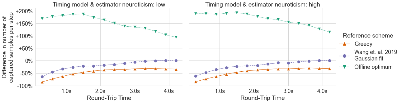
The results of this investigation are presented in Figure 12, and clearly show the advantages of using the sample-count-optimized scheme over the current state-of-the-art. The performance of [21]’s approach appears to degrade with lower RTT, exponentially oversampling as latency tends to zero and the maximum sampling rate of the system tends to infinity. On the other hand our sampling scheme consistently matches or beats the state-of-the-art while maintaining a relatively constant behavior with respect to RTT. As mentioned above, the future feasibility and mass adoption of WCA depends on these applications not hogging the available resources. Our work advances this goal by being consistently more efficient than existing alternatives at minimizing the number of samples per step, and thus reducing network and processing load.
It should be noted that although both schemes seem to tend towards two samples per step as RTT increase, this is simply an artifact of our experimental setup. As RTT increase above the expected wait time, the probability of the sum of the first sampling interval and the RTT being larger than the execution time of the step tends towards . This leads to these sampling schemes consistently sampling only twice each step: a first sample which is taken before the execution time of the step, and a second one RTT seconds later, after the execution time has been reached.
VI-C Optimizing for energy consumption
Next we will explore the implications of combining our timing models with Equation 4 when directly optimizing for energy consumption in WCA. Although, as mentioned above, minimizing the number of samples captured during a step can potentially translate into a reduction in the energy consumption, this is not a given. Energy consumption depends on multiple other factors other than number of samples captured, such as idle versus communication power and delays, and thus cannot be optimized by simply minimizing the number of samples taken.
In the following, we thus take the general solution, Equation 4, and find the appropriate and to minimize the energy consumed per step, i.e. . We directly take the modeling from [26] with a necessary modification in the assumption of one-way communication in all but the final sample. With feedback given even to the discarded samples in our model and communication delay defined as the total delay in either direction, we have,
| (8) |
and correspond to the processing and two-way communication delay for each sample. and correspond to the communication and idle power, respectively, of the WCA client device.
We proceed to repeat the experiment detailed in Section VI-B, replacing the sample-count-optimized sampling scheme with a new implementation instead minimizing energy, using Equation 8 for the calculation of and . Once again, we embed a timing model into the sampling scheme to provide updated estimates of the mean execution time at each step. We refer to this scheme as the energy-optimized aperiodic sampling scheme. For the power constants, we reuse the values estimated by the authors in [25], and . On the other hand, for the timing variables we define a constant processing delay across all configurations and repetitions of the experiments; given then a constant RTT for the task, we set .


Again, we include the reference greedy and offline optimum schemes, as well as [21]’s approach, and repeat the experiment times for each combination of sampling scheme, neuroticism, and RTT.
The results of these experiments are presented in Figure 13, and they clearly illustrate the advantages of the integration of our timing models with an adaptive, energy-optimized sampling scheme when compared to unoptimized and state-of-the-art sampling schemes. Our approach is consistently consumes less energy than [21]’s state-of-the-art, and is up to more energy efficient than the greedy scheme. Furthermore, once again the behavior of our approach is more consistent and reliable than the competition, exhibiting a flat curve of energy consumption much akin to that of the offline optimum in behavior.
VII Conclusion
This paper addresses the difficulty of benchmarking WCA by offering a model-based alternative to the extensive human-user studies that would otherwise be required. It first introduces the EdgeDroid model of human timing behavior for WCA. This model represents a stochastic approach to execution time modeling which builds upon prior data [9]. It further introduces a novel procedure for the generation of synthetic traces of frames in step-based WCA, allowing for a full end-to-end emulation of a human when combined with the timing model.
The paper then explores the impact of such a realistic model on the application lifetime footprint of WCA applications. It shows that less realistic modeling approaches which do not take into account higher-order effects on execution time distributions, can potentially lead to substantial mis-estimations of the application footprint.
Finally, the paper delves into the potential for optimization in WCA systems using the previously discussed timing models. It proposes a novel stochastic optimization framework for resource consumption-system responsiveness trade-offs in WCA, which results in an adaptive sampling strategy. We have shown that this framework is applicable to both the minimization of number of samples and total energy consumption per step by showcasing experimental results. Our results show up to a increase in performance with respect to state of the art when optimizing for number of samples, and up to a improvement when optimizing for energy consumption, thus proving the value of such frameworks for the design of WCA applications.
This work serves as an important, yet initial step towards realistic modeling of human behavior in WCA, and more generally AR. Many directions remain open to additional exploration in this space. For instance, our current model only targets a particular class of step-based WCA, and extension of our methodology to other classes of these applications, or even more generally to AR and XR, is on our roadmap. Our data [9] also only considers young undergraduate students at a highly competitive university in the United States. An extension of this dataset and the model towards a more representative sample of the general population would surely be a valuable endeavor. Corresponding research is needed to determine individual difference factors that would substantially impact response to WCA in novel populations.
In terms of the optimization framework, our current model adopts the assumption that execution times are Rayleigh-distributed. Although this distribution fits the data reasonably well, there are other which more accurately describe the behavior of human execution times (e.g. the exGaussian). Our future efforts consider developing this framework towards these more accurate distributions. Finally, our current approach only considers a single client, which will be far from the case in a real-world WCA deployment. As such, another milestone in this context could be the exploration for a potential extension towards a collaborative and/or distributed solution.
Acknowledgements
This work has been partially funded by the SSF (SSF) (grant number ITM17-0246 (ExPECA)), and the NSF (NSF) (grant number CNS-2106862).
The funders had no role in study design, data collection and analysis, decision to publish, or preparation of the manuscript.
Any opinions, findings, conclusions or recommendations expressed in this material are those of the authors and do not necessarily reflect the view(s) of their employers or funding sources.
References
- [1] Mahadev Satyanarayanan et al. “The case for vm-based cloudlets in mobile computing” In IEEE pervasive Computing 8.4 IEEE, 2009, pp. 14–23
- [2] Kiryong Ha et al. “Towards Wearable Cognitive Assistance” In Proceedings of the 12th Annual International Conference on Mobile Systems, Applications, and Services, MobiSys ’14 Bretton Woods, New Hampshire, USA: Association for Computing Machinery, 2014, pp. 68–81 DOI: 10.1145/2594368.2594383
- [3] Mahadev Satyanarayanan and Nigel Davies “Augmenting cognition through edge computing” In Computer 52.7 IEEE, 2019, pp. 37–46 DOI: 10.1109/MC.2019.2911878
- [4] Markus Funk and Albrecht Schmidt “Cognitive assistance in the workplace” In IEEE Pervasive Computing 14.3 IEEE, 2015, pp. 53–55
- [5] Zhuo Wang et al. “A comprehensive review of augmented reality-based instruction in manual assembly, training and repair” In Robotics and Computer-Integrated Manufacturing 78 Elsevier, 2022, pp. 102407
- [6] Zhuo Chen et al. “An empirical study of latency in an emerging class of edge computing applications for wearable cognitive assistance” In Proceedings of the Second ACM/IEEE Symposium on Edge Computing, 2017, pp. 1–14
- [7] Cl\’ement Belletier et al. “Wearable cognitive assistants in a factory setting: a critical review of a promising way of enhancing cognitive performance and well-being” In Cognition, Technology & Work 23.1 Springer, 2021, pp. 103–116
- [8] Zhuo Chen “An application platform for wearable cognitive assistance”, 2018 URL: https://elijah.cs.cmu.edu/DOCS/CMU-CS-18-104.pdf
- [9] Manuel Olguínñoz et al. “Impact of delayed response on wearable cognitive assistance” In PLOS ONE 16.3 Public Library of Science, 2021, pp. 1–25 DOI: 10.1371/journal.pone.0248690
- [10] Manuel Olgu\’n\˜noz et al. “Scaling on the Edge–A Benchmarking Suite for Human-in-the-Loop Applicationss” In 2018 IEEE/ACM Symposium on Edge Computing (SEC), 2018, pp. 323–325 IEEE
- [11] Manuel Osvaldo Olgu\’n\˜noz et al. “EdgeDroid: An experimental approach to benchmarking human-in-the-loop applications” In Proceedings of the 20th International Workshop on Mobile Computing Systems and Applications, 2019, pp. 93–98
- [12] Shilpa George et al. “OpenRTiST: end-to-end benchmarking for edge computing” In IEEE Pervasive Computing 19.4 IEEE, 2020, pp. 10–18
- [13] Yongcheng Jing et al. “Neural style transfer: A review” In IEEE transactions on visualization and computer graphics 26.11 IEEE, 2019, pp. 3365–3385
- [14] Mattia Lecci et al. “An Open Framework for Analyzing and Modeling XR Network Traffic” In IEEE Access 9 IEEE, 2021, pp. 129782–129795
- [15] Sofiane Chetoui et al. “ARBench: Augmented Reality Benchmark For Mobile Devices” In 2022 IEEE International Symposium on Performance Analysis of Systems and Software (ISPASS), 2022, pp. 242–244 IEEE
- [16] Brian Cooper et al. “Benchmarking cloud serving systems with YCSB” In Proceedings of the 1st ACM symposium on Cloud computing, 2010, pp. 143–154
- [17] Zhen Jia et al. “Characterizing data analysis workloads in data centers” In 2013 IEEE International Symposium on Workload Characterization (IISWC), 2013, pp. 66–76 IEEE
- [18] Anirban Das et al. “Edgebench: Benchmarking edge computing platforms” In 2018 IEEE/ACM International Conference on Utility and Cloud Computing Companion (UCC Companion), 2018, pp. 175–180 IEEE
- [19] Jonathan McChesney et al. “Defog: fog computing benchmarks” In Proceedings of the 4th ACM/IEEE Symposium on Edge Computing, 2019, pp. 47–58
- [20] Sadagopan Srinivasan et al. “Performance characterization and optimization of mobile augmented reality on handheld platforms” In 2009 IEEE International Symposium on Workload Characterization (IISWC), 2009, pp. 128–137 IEEE
- [21] Junjue Wang et al. “Towards scalable edge-native applications” In Proceedings of the 4th ACM/IEEE Symposium on Edge Computing, 2019, pp. 152–165
- [22] Zhaohui Huang and Vasilis Friderikos “Proactive edge cloud optimization for mobile augmented reality applications” In 2021 IEEE Wireless Communications and Networking Conference (WCNC), 2021, pp. 1–6 IEEE
- [23] Ali Al-Shuwaili and Osvaldo Simeone “Energy-efficient resource allocation for mobile edge computing-based augmented reality applications” In IEEE Wireless Communications Letters 6.3 IEEE, 2017, pp. 398–401
- [24] Vishnu Moothedath et al. “Energy-Optimal Sampling of Edge-Based Feedback Systems” In IEEE International Conference on Communications Workshops (ICC Workshops), 2021, pp. 1–6 DOI: 10.1109/ICCWorkshops50388.2021.9473894
- [25] Vishnu Moothedath et al. “Energy Efficient Sampling Policies for Edge Computing Feedback Systems” In IEEE Transactions on Mobile Computing, 2022, pp. 1–1 DOI: 10.1109/TMC.2022.3165852
- [26] Vishnu Moothedath “Energy-Optimal Sampling for Edge Computing Feedback Systems: Aperiodic Case (To be published)” In IEEE/ACM Symposium on Edge Computing (SEC), 2022, pp. 403–408
- [27] Zhuo Chen et al. “Early Implementation Experience with Wearable Cognitive Assistance Applications” In Proceedings of the 2015 Workshop on Wearable Systems and Applications, WearSys ’15 Florence, Italy: Association for Computing Machinery, 2015, pp. 33–38 DOI: 10.1145/2753509.2753517
- [28] Oliver John and Sanjay Srivastava “The Big Five trait taxonomy: History, measurement, and theoretical perspectives” In Handbook of personality: Theory and research 2.1999, 1999, pp. 102–138
- [29] Bob Witmer and Michael Singer “Measuring presence in virtual environments: A presence questionnaire” In Presence 7.3 MIT Press, 1998, pp. 225–240
- [30] Jacob Hirsh et al. “Delay discounting: Interactions between personality and cognitive ability” In Journal of research in personality 42.6 Elsevier, 2008, pp. 1646–1650
- [31] Frank Massey “The Kolmogorov-Smirnov test for goodness of fit” In Journal of the American statistical Association 46.253 Taylor & Francis, 1951, pp. 68–78
- [32] Doug Rohrer and John Wixted “An analysis of latency and interresponse time in free recall” In Memory & Cognition 22.5 Springer, 1994, pp. 511–524
- [33] Evan Palmer et al. “What are the shapes of response time distributions in visual search?” In Journal of experimental psychology: human perception and performance 37.1 American Psychological Association, 2011, pp. 58
- [34] Fernando Marmolejo-Ramos et al. “Generalised exponential-Gaussian distribution: a method for neural reaction time analysis” In Cognitive Neurodynamics Springer, 2022, pp. 1–17
- [35] Fukumoto Satoshi et al. “Optimal Checkpointing Policies Using the Checkpointing Density” In Journal of Information Processing 15.1, 1992, pp. 97–92
- [36] Richard Bellman “Dynamic programming and a new formalism in the calculus of variations” In Proceedings of the National Academy of Sciences of the United States of America 40.4 National Academy of Sciences, 1954, pp. 231
- [37] George Arfken et al. “Calculus of Variations”, 2013, pp. 1081–1124
In this appendix, we give the mathematical derivation of the optimum aperiodic sampling interval discussed in Section VI-A. We start with the general solution, where the objective function to be minimized is given by Equation 4:
We first borrow the idea of checkpointing density from [35] and define an instantaneous sampling rate function which is related to such that,
| (9) |
Note that, for periodic sampling, this function is a constant, equal to the sampling frequency. In the aperiodic case, we find , the that minimizes . By construction, the number of samples taken up to any time instant can be computed directly by computing the area under . Thus, we obtain the expected number of samples as
| (10) |
To find , we use the conditional CDF of the execution time.
The numerator is degenerate when or . Thus, we are only interested in . Let , and correspond to the CDF, CCDF (CCDF) and PDF (PDF) of the execution time distribution.
| (11) |
Here, Equation 11 is an approximation merely for mathematical maturity due to the slackness of the first inequality in the numerator. We expand and using Taylor series. Thus we can write the CCDF as
Simplifying and approximating by ignoring the higher order terms, we arrive at
| (12) | ||||
Next, using the above CCDF, we find the conditional expectation of .
If is varying slowly between two consecutive sampling instants due to the closeness of two sampling intervals, we can approximate the sampling interval as
| (13) | ||||
| (14) |
We can thus find the energy penalty using Equation 10 and Equation 14 as
| Let . Then . That is, | ||||
As per the Euler-Lagrange equation from the calculus of variations [36, 37], the extreme value of is obtained at
| (15) | ||||
| Thus, for a Rayleigh distributed with parameter , | ||||
| (16) | ||||
| (from (9)) | ||||
| We have . Substituting , in order, in the above equation provides us our final result | ||||
| (17) | ||||
Note that, due to the close similarity in their density functions, the task times can be approximated fairly equally to an exGaussian distribution as well as a Rayleigh distribution, with the former attracting more attention from works like [32, 33, 34]. This is the reason why the above results are applicable in this work where we have predominantly considered exGaussian distribution. Furthermore, we have also verified the closeness of the results as well as the validity of the approximations made in the proofs using distribution fitting and simulations.
By making use of this general solution, we can also prove the results given in Section VI-B, where we modify the problem and find the optimum sampling instants that minimize the expected number of samples for a given upper bound for the expected wait time. First note that the general solution has constants and corresponding to the weights given to the cost of sampling and waiting, respectively. The optimization criteria changes from minimizing wait time to minimizing the number of samples when the ratio goes from zero to infinity. Since any positive real value is valid for this ratio, one can achieve any valid point via simply by varying the ratio .
Furthermore, since the sampling instants are aperiodic and can take any positive real values, the bound will be tight at the optimum. Hence, to solve for the modified optimization problem explained in Section VI-B that minimizes with an upper bound on , we equate Equation 14 to , find the corresponding , and find the optimum set of sampling instants by plugging this ratio into Equation 17.
| where is the gamma function. Thus, when the upper bound is tight, | ||||