Hybrid Censored Quantile Regression Forest to Assess the Heterogeneous Effects
Abstract
In many applications, heterogeneous treatment effects on a censored response variable are of primary interest, and it is natural to evaluate the effects at different quantiles (e.g., median). The large number of potential effect modifiers, the unknown structure of the treatment effects, and the presence of right censoring pose significant challenges. In this paper, we develop a hybrid forest approach called Hybrid Censored Quantile Regression Forest (HCQRF) to assess the heterogeneous effects varying with high-dimensional variables. The hybrid estimation approach takes advantage of the random forests and the censored quantile regression. We propose a doubly-weighted estimation procedure that consists of a redistribution-of-mass weight to handle censoring and an adaptive nearest neighbor weight derived from the forest to handle high-dimensional effect functions. We propose a variable importance decomposition to measure the impact of a variable on the treatment effect function. Extensive simulation studies demonstrate the efficacy and stability of HCQRF. The result of the simulation study also convinces us of the effectiveness of the variable importance decomposition. We apply HCQRF to a clinical trial of colorectal cancer. We achieve insightful estimations of the treatment effect and meaningful variable importance results. The result of the variable importance also confirms the necessity of the decomposition.
keywords
Random Forest, Quantile Regression, Survival Analysis, Heterogeneous effects1 Introduction
Precision medicine and individualized health care are a future direction of medicine to optimize health benefits for all. To achieve that, one needs to have a thorough understanding of heterogeneous treatment effects in a target population. More and more studies (e.g., Kravitz et al. 2004; Kosorok and Moodie 2015) suggest that the effect of a drug or an intervention could depend on individuals’ health conditions, medical history, genetic profiles, and many other factors. Hence, it would be desirable to assess the heterogeneous treatment effect incorporating high-dimensional covariates. In this paper, we focus on censored time-to-event outcomes, a family of widely-considered outcomes in health analyses and risk modeling.
Estimating the heterogeneous effects potentially varied with a large number of covariates for the censored data brings many challenges. Besides the curse of dimensionality, the effect function is likely to be an unknown function of covariates. The naive estimation approaches, such as the linear additive model with treatment-covariate interaction effects, may oversimplify the complexity of response-covariate associations in reality. Recent advancements in machine learning methods make it possible to model nonlinear and complex associations with high-dimensional covariates. Among them, random forest is a popular choice due to its competitive prediction accuracy and feature selection, which are important considerations for health applications.
Random forest (Breiman 2001) is an ensemble of regression and classification trees constructed from recursive partitions. The partitions separate dissimilar subjects by a specific splitting criterion, resulting in homogeneous subgroups in terminal nodes. The nonparametric nature of the recursive partition framework makes random forest adept to high-dimensional covariates, and complex and nonlinear associations. It hence becomes a powerful tool for prediction and is widely used across many fields. Several random forest approaches were developed for time-to-event outcomes. Ishwaran et al. 2008 introduced the random survival forest to estimate the cumulative hazard function by averaging the Nelson-Aalen estimator of the terminal node where the individual locates in each tree of the random forest. Zhu and Kosorok 2012 used extremely randomized trees and proposed an imputation procedure that recursively updates the censored observations. Steingrimsson et al. 2019 extended the censoring unbiased transformation to squared error loss functions and proposed a new recursive partition approach based on it. The target function in the above approaches is the conditional survival or conditional cumulative hazard function. Hothorn et al. 2006 proposed a random forest to estimate the conditional mean of the log–survival time. Li and Bradic 2020 extended the quantile forest (Athey et al. 2019) with a loss function adept to the censored data to estimate the quantile of the survival time. The aforementioned random forests are powerful tools for risk prediction, but they are not designed to assess the heterogeneous covariates effects on the censored outcome.
In this paper, we propose a forest-based estimation procedure to assess the heterogeneous effects of the covariates for right-censored data. The proposed hybrid censored random forest integrates the censored quantile regression with the random forest. The estimation procedure based on it enables us to estimate the heterogeneous effects of the covariates at a quantile level of interest. It is a doubly-weighted estimation framework, which comprises a redistribution-of-mass weight (Wang and Wang 2009) to handle censoring and an adaptive nearest neighbor weight derived from the forest to handle high-dimensional effect functions. The proposed forest algorithm is based on a two-step splitting rule by evaluating the heterogeneity of the coefficients and goodness-of-fit of a quantile regression model. An inference-based criterion is used to choose the splitting variable. A loss-function-based criterion is used to select the splitting value.
The main contributions of the proposed approach are as follows. First, the proposed approach models the survival time directly by a censored quantile regression, which results in a relevant interpretation of the estimation and also provides an opportunity to assess the future risk based on the estimated model. Second, it expands the utility of the classical random forest to assess the heterogeneous effects of the covariates potentially varying with high-dimensional variables. The perspective of viewing a random forest as an adaptive kernel approach (Lin and Jeon 2006; Meinshausen 2006; Athey et al. 2019) is widely adopted. However, the estimated nonparametric regression functions derived by those approaches cannot directly evaluate the heterogeneity of the covariate effects, which is of great need in many medical applications. The proposed hybrid approach is able to help us understand the effects varying by individuals and relieves the restriction of the specific structure assumption of effects functions in other estimation approaches. Third, we propose a two-step splitting rule in the random forest, avoiding favoring variables with more possible splits. Last but not least, the mutually advantageous conjunction of the quantile regression model and random forest allows us to tackle all the challenges in assessing the heterogeneous effects with high-dimension.
The rest of the paper is organized as follows. In Section 2, we introduce the censored quantile regression model with heterogeneous coefficient functions. In Section 3, we present the estimation procedure of the heterogeneous coefficient functions obtained by the proposed hybrid forest. Details about how the hybrid forest is built are given in Section 4. In Section 5, we conduct a variety of simulation experiments to evaluate the estimation performance of the proposed approach and compare it with other approaches. The proposed method is illustrated with the analysis of a randomized phase III study in Section 6 with some discussions.
2 Censored Quantile Regression Model with Heterogeneous Coefficient Functions
Let be a survival time outcome. We denote by a -dimensional vector of predictive variables including a constant , whose effects on the quantiles of are of interest, and denote by a -dimensional vector of modifiers (Hastie and Tibshirani 1993), which potentially modify the effects of . Defining as the conditional quantile function of given at the quantile level , we consider the following quantile regression model
| (1) |
where is the effect of on the th quantile of , and is an unknown function of . Since includes a constant 1, the coefficient function includes both the intercept function and the slope functions .
The choice of depends on specific applications. For example, when the predictive variable is a binary indicator of treatment, is the individualized quantile treatment effect (QTE) given the covariates . When the predictive variable is a continuous dose variable, outputs a heterogeneous dose-response relationship that could vary by . There are also applications where the choice of predictive variables is informed by domain knowledge. In Model (1), the dimension of can be high and grow with the sample size, while the dimension of is low and fixed. This way, we could fully capture individualized heterogeneous quantile effect , and ensure its estimation is feasible.
In this paper, we assume that the survival time is subject to right censoring, and the censoring time, denoted by , is independent of conditional on . In the presence of censoring, we observe the censored time and the event indicator . Throughout the paper, we denote a censored random forest by , where refers to the th tree in the forest.
3 Doubly-weighted Estimation From A Censored Forest
In Model (1), if the coefficient function is a constant, Model (1) reduces to a simple linear quantile regression of the survival time and its predictors . On the other hand, if only includes the constant 1, Model (1) reduces to a nonparametric quantile regression model. The latter can also be estimated by existing censored random forests (i.e., Li and Bradic 2020). In this section, we are going to propose a doubly-weighted estimation approach to estimate in Model (1).
If the dimension of covariates is low, Model (1) shares the same form as a varying-coefficient model without censoring, and the estimation of can be carried out through kernel smoothing or spline approximation (Hastie and Tibshirani 1993; Honda 2004; Cai and Xu 2009). Those approaches are not scalable for high dimensions. To estimate in Model (1) with high-dimensional and censored outcome, we propose a doubly-weighted hybrid estimation procedure in conjunction with censored quantile regression and random forest. In this section, we assume that a forest is available.
3.1 Forest-based Weights
We start by estimating using uncensored data. Our approach to estimate the quantile coefficient function for a given relies on a similarity weights , where measures the contribution of the th sample in estimating . To accommodate the high-dimensional , we propose to use a random forest to construct the similarity weights as in Meinshausen 2006 and Athey et al. 2019. In what follows, is termed forest-based weight. Suppose we have a random forest of trees, indexed by . In each tree , we denote by the terminal node that contains . The forest-based weights is then defined as,
| (2) |
where is the number of observations in the terminal node . In each tree , if is contained in the terminal node , it contributes towards estimating with weight . Otherwise, its weight is zero. The weight is obtained by aggregating over trees. It is easy to see that , and the weights define an adaptive neighborhood of identified by the random forest.
In the absence of censoring, one can estimate the quantile coefficient function by minimizing weighted quantile loss
| (3) |
where is the quantile loss function.
3.2 Redistribution Weights
In the presence of censoring, the quantile loss in (3) can no longer be used. Instead, we consider a weighted quantile regression with redistribution weights suggested in Wang and Wang 2009 when censoring exists. The weighted quantile loss can be written as
| (4) |
where is any value sufficiently large to exceed all . The redistribution weights in (4) are defined as
| (5) |
where is the conditional cumulative distribution function of given . The conditional cumulative function is unknown. In practice, we can use proper estimation approaches to obtain the estimated .
The redistribution weights root from a unique property of the quantile regression, whose estimator is only determined by the signs of residuals. By design, the redistribution weight if is either an observed event time or the conditional censoring probability given is larger than . In both cases, the sign of the residual is determined. Hence it contributes towards the quantile estimate as a full observation. However, when is censored, and the conditional censoring probability is smaller than , the sign of becomes undetermined. In this case, assign the probability mass to a sufficiently-large value, and “redistribute” the remaining probability by .
Combining the forest-based weights (2) together with the redistribution weight (5), we could estimate at a fixed and a fixed quantile level from a random forest by
| (6) |
In the above discussion, we assume a forest is available. In what follows, we consider a censored quantile random forest algorithm to build the forest.
Remark 1.
For censored outcomes, many researchers have considered modeling the quantiles under linear assumptions. Powell 1984 and Powell 1986 proposed a linear quantile regression model under fixed censoring. Portnoy 2003 introduced a weighted estimation approach exploiting the idea of redistribution-of-mass. Peng and Huang 2008 proposed a martingale-based estimating procedure. Both Portnoy 2003’s and Huang et al. 2002’s approaches relied on a global linear assumption at all quantile levels. De Backer et al. 2019 introduced a new loss function tackling the censoring based on the conditional distribution of the survival and the observed time. However, the computation of the adapted majorize-minimize algorithm is complex. Leng et al. 2013, and Xie et al. 2015 employed inverse probability weighting (IPW) to handle the censoring. Such IPW approaches are often unstable when some estimated propensity scores are too small. We consider the redistribution weights suggested in Wang and Wang 2009 due to its relaxed linear assumption and simple minimizing algorithm. The redistribution weight is controlled as , and hence avoids the risk of variance inflation.
4 Hybrid Censored Quantile Regression Random Forest
In this section, we propose a hybrid censored random forest, where we incorporate the censored quantile regression in the partition algorithm. Instead of the heterogeneity of the conditional mean or quantile (Meinshausen 2006; Athey et al. 2019), the proposed partition algorithm aims to identify and differentiate the heterogeneity of the function in Model (1) in the covariate space. In each node, we intend to search for the most effective modifier of the coefficient function in Model (1) by the proposed splitting criterion.
Following the convention in random forest (Breiman 2001), we denote as the collection of all possible binary split rules determined by a single modifier in and a cut-off value, where is denoted as a collection of some observations in a node. We denote by the sample size of the node. We also denote by and the left and right child nodes respectively based on a split . Consequently, and .
A greedy search over might favor a continuous splitting variable, because it has many more possible splits (Loh 2014). To avoid such selection bias and reduce the computation burden, we consider a two-step splitting algorithm, where we first use a re-distributed rank statistics to select the best splitting variable that maximizes the marginal heterogeneity in . Once the splitting variable is chosen, we search for a split that optimizes the goodness-of-fit of Model (1). Details of the algorithm are given in Algorithm 1.
4.1 Re-distributed Rank-score for Choosing Splitting
When choosing an optimal splitting variable, we consider a screening procedure to search for the most effective modifier of in a parent node . We use an indicator function to indicate where the observation locates according to the split : if and otherwise. We propose to use a rank-based statistics to find the optimal splitting variable. We first consider when we can observe complete data. For Model (1) without censoring, there is no direct approach to identify the most effective modifier in an unknown function . Instead, we rely on a working model , for each . The rank-based test is well defined for testing the null hypothesis . Even if the working model is misspecified, it is still natural to choose the variable with the largest rank-score statistics as a splitting variable (Loh 2002). The rank-based statistics will make the selection procedure simple and efficient. However, the regression rank score for censored quantile regression is not well defined.
The following outlines how we obtain the rank-based statistics to choose the optimal variable in the node without censoring. We let and be the design matrix of Model (1) and the matrix of modifiers correspondingly in the node , and be the th column in . The quantile loss function in the node is,
| (7) |
where function is defined in (3). We let be a column vector with th element being the regression rank-score (Hájek 1965) for the quantile regression (Koenker 2005),
| (8) |
where is the sample minimizer of . Then let be the interaction matrix between the predictive variables and the th modifier and is a diagonal matrix with being the diagonal elements. The projection of the interaction matrix to the spanned column space of is where .
Then, the rank score statistics to evaluate the heterogeneity of the quantile coefficients induced by the th modifier is
| (9) |
where and . Intuitively, only depends on the signs of and hence it represents the relative positions of after adjusting for at th quantile in the node . A smaller value of the norm of means that no variation in can be further explained by . Thus, a larger value of implies that more variation in can be explained by the interaction . In the presence of censoring, we follow Sun 2020 and replace with , where is the redistribution weight (5). The expectation of the new regression rank score with censoring equals to the one without censoring. Thus, with is an approximation of the rank test statistics for uncensored data, and hence we choose the modifier with the largest value of as the splitting variable.
Once the splitting variable is chosen, we seek a cut-off value that improves the fitting of the trees as much as possible. Denote by the minimizer of . The optimal split is given by
| (10) |
where is the collection of all possible binary split rules determined by the selected splitting variable and a cut-off value in the node . It can be shown that splitting generally improves the loss function, that is, for any split , we have .
4.2 Variable Importance
Variable importance is often used as a reference to measure the prediction strength of each variable in the data set. In our framework, we are further interested in the effective modifiers of the quantile coefficient function. We propose two types of permutation-based variable importance. The first one evaluates the overall impact of a modifier in the conditional quantile of the response variable. The second one measures the impact of a modifier on the treatment effect when the predictive variable is a binary treatment variable.
We first introduce how we obtain the variable importance to evaluate the overall prediction strength. We denote the original data set by . Once the random forest has been grown, we follow the procedure of permutation importance (Breiman 2001) and calculate the variable importance for th variable with the following steps,
- 1.
estimate the quantile loss in based on : , where is the estimated quantile coefficient estimated by (6) but with those trees where is in the out-of-bag samples;
- 2.
generate a new data set by shuffling the th modifier randomly, where is a vector of modifiers for th observation with th element being the value after permutation and other elements being the same as in ;
- 3.
calculate the quantile loss in the new data set based on : , where is the value of at ;
- 4.
repeat 2-3 times (e.g., ) and the variable importance of th modifier is: .
With the above procedure, we can obtain the variable importance for each modifier . The permutation step (step 2) breaks any association between th modifier and the response. Thus, the difference of quantile losses before and after the permutation step measures the overall prediction strength of the th modifier. However, sometimes, the overall importance is manifested by the prediction strength in the main effect while the one in is of our interest. Therefore, we propose the second variable importance, which measures the predictive strength of the th modifier in when the predictive variable is a binary treatment variable.
If is a binary variable, then contains two functions, the intercept function and the slope function . It is of primary interest to identify effective modifiers in . We propose a variable decomposition which decomposes the variable importance score into two parts by different values of to discriminate the importance for and . The overall variable importance can be decomposed into the importance score for and the one for . We assume that the treatments are randomly assigned and hence define the variable importance given as,
| (11) | ||||
When , is the importance score of th modifier in . When , we have . The variable importance contains both the importance score of th modifier for both and . Therefore, intuitively, the variable importance for can be calculated by .
If does not vary with the change of th modifier, the difference of the variable importance scores between two groups, should be close to . A value of being away from 0 possibly indicates that changes with th modifier. Both positive and negative values of the difference provide evidence for the interaction effect of the treatment and the modifier. Thus, we use the absolute value of the difference between the two importance scores to evaluate the impact of a modifier on the treatment effect.
4.3 Computation Algorithm
The proposed ensemble procedure is summarized in Algorithm 1.
The candidacy of a node for splitting: the number of observations of is larger than the pre-specified number MINSPLIT.
4.4 Computation Specification
In the simulation and real data analysis, when calculating the redistribution weights (5), we need to obtain the conditional cumulative distribution function of the survival time given : . In practice, is unknown. A variety of attempts have been made to estimate it. To name a few, Portnoy 2003 suggested estimating through fitting an entire quantile regression process under the global linearity assumption of the conditional quantile functions. McKeague et al. 2001 tried to fit a semiparametric model (e.g., Cox proportional hazard model) to obtain an approximation of . Wang and Wang 2009 proposed a fully nonparametric approach based on a local Kaplan-Meier estimator to estimate . The parametric and semiparametric approaches endure strong linearity assumptions, which is sometimes not practical. Furthermore, the nonparametric approach is only feasible when the dimension of covariates is small. Later, Wang et al. 2013 proposed to perform a global dimension reduction formulation to facilitate the local weight estimation for multivariate covariates. Albeit it makes the nonparametric adapted to multivariate covariates, the dimension reduction formulation may lead to the loss of information. The kernel-based nonparametric approach is restricted to the types of covariates (e.g., when both continuous and categorical covariates exist). In order to relieve the restrictions of the previous approaches, we propose to estimate by the random survival forest (RSF, Ishwaran et al. 2008). By taking advantage of the random forests, the estimator by RSF is able to accommodate both continuous and categorical covariates and bypasses the restriction of types of covariates. The estimated conditional cumulative distribution function of , denoted by , takes the place of in (5).
We also point out other computing specifications as follows,
- 1.
We set the total number of trees in the forest as , the minimal number of samples in a terminal node is MINSPLIT, the subsampling rate is , and the number of randomly selected splitting variables at each split is .
- 2.
When optimizing the loss function in (6), we suppose that among observations, the first survival times are censored, and the remaining are observed. When estimating the quantile coefficient, we append to , where is a sufficiently large number and when implemented in computation, we let . Then we can simply use the function
rqinRpackagequantregwith the corresponding weight or to obtain the estimated quantile coefficient. - 3.
The random survival forest to estimate the conditional distribution was implemented by the function
rfsrcin the R packagerandomForestSRCwith default settings.
5 Simulation
In this section, we present simulation studies to evaluate the finite sample performance of the proposed HCQRF with comparisons of the following alternative methods.
-
Censored Quantile Regression Forest (Li and Bradic 2020, CQRF,): CQRF is an extension of generalized random forest (Athey et al. 2019, grf,) but tailored for censored data. It treats both and equally as splitting variables, and is designed to estimate the conditional quantile function . When is binary, one can estimate .
-
HCQRF-complete (HCQRF-c): We apply the proposed HCQRF on the complete data without censoring (i.e., we use the simulated data before introducing censoring such that all the ’s are fully observed).
-
grf-complete (grf-c): We also construct CQRF from the complete data, but use the proposed double-weighed approach to estimate the coefficient function from the resulting random forest. Since the double-weighting estimation scheme by (6) is valid when is not included as the splitting variables, and only are used as splitting variables. We denote this approach as grf-c, as it is in the essence of generalized random forest, which views random forest as a way to generate adaptive kernels (2) (Lin and Jeon 2006; Scornet 2016).
We summarize the key differences across those approaches in Table 1. Among those comparison methods, CQRF is a popular existing random forest approach for censored quantiles. By comparing HCQRF and CQRF, we evaluate the estimation performance in the context of the latest literature. On the other hand, HCQRF-c serves as a benchmark approach. We compare HCQRF to HCQRF-c to assess the impact of censoring. By design, the main difference between HCQRF-c to grf-c is the choice of splitting rules. Although grf-c is not an existing approach, we include it as one of the comparison methods, and compare HCQRF-c to grf-c to illustrate the value and need of the proposed splitting rules when it comes to estimating heterogeneous treatment effects. Specifically, in Sections 5.2 and 5.3, we evaluate their performance in estimating the coefficient functions under various scenarios. Since CQRF can only estimate for binary , we compare its performance in estimating the conditional quantile function with the proposed HCQRF, and the results are presented in Section 5.4. Finally, we present a simulation study in Section 5.5 to assess the effectiveness of the proposed variable importance decomposition in feature selection.
5.1 Simulation Settings
We design the simulation scenarios with the following survival model
| (12) |
where and are functions of effect modifiers , and is an error term. In the Sections 5.2 and 5.3, we outline the specifics of the distributions of and , the functions and , and the distribution of under each scenario. In the meantime, we generate both completely random and covariate-dependent censoring time. The censoring rate in the following simulation scenarios is approximately 25% at . Thus, the observed time is , and the censoring status is .
In each Monte Carlo repetition, we generated a data set, , on which the random forest is built based. We consider two sample sizes, and . We evaluate the estimation performance based on a new data set, , which is generated independently in each Monte Carlo repetition following the same generation mechanism. We let . We assessed the performance in estimation by the mean squared error (MSE), and mean absolute error (MAE) of both the estimated quantile coefficient function and the estimated quantile functions. Specifically, for each Monte Carlo simulation, we calculate
| (13) |
where is the estimated quantile coefficient function and is the true one. In the Supplementary Materials, we also demonstrate the relative mean squared error (RMSE) and relative mean absolute error (RMAE) as additional scale-free assessments of the estimation performance.
| Method | Outcome used | Splitting rule | Splitting variables | Estimate | Estimate |
|---|---|---|---|---|---|
| HCQRF | Censoreda | Comparing conditional quantiles of given between the left and right child nodes | By minimizing the objective function in (6) with random forest weight (2) | ||
| CQRF | Censored | Comparing the marginal quantiles of between the left and right child nodesc | and | Unable to estimate directlyd | |
| HCQRF-c | Completely observed | The same as HCQRF | The same as HCQRF | ||
| grf-c | Completely observed | Comparing the marginal quantiles of between the left and right child nodes | The same as HCQRFf |
- a
The censored data is used.
- b
The complete data is used.
- c
The splitting rule is directly applied on censored data without adjustment of the censoring.
- d
If the predictive variable is a binary variable, the coefficient function can estimated by and .
- e
We abbreviate as .
- f
CQRF applying on the complete data is in the essense of grf (Athey et al. 2019), which is not able to estimate directly. We can obtain the estimated by following the same double-weighting estimation scheme (6) with forest weight (2) generated by grf.
5.2 Estimation Accuracy
In this subsection, we present a simulation study to assess and compare HCQRF, CQRF, HCQRF-c and grf-c in estimating the coefficient functions under various scenarios. We start with a simple scenario (Scenario 2), where is binary, and its quantile coefficient is a piece-wise constant function of . In Scenarios 3 and 4, we considered continuous and with non-linear and continuous coefficient functions. Figure 1 displays the under the three scenerios.
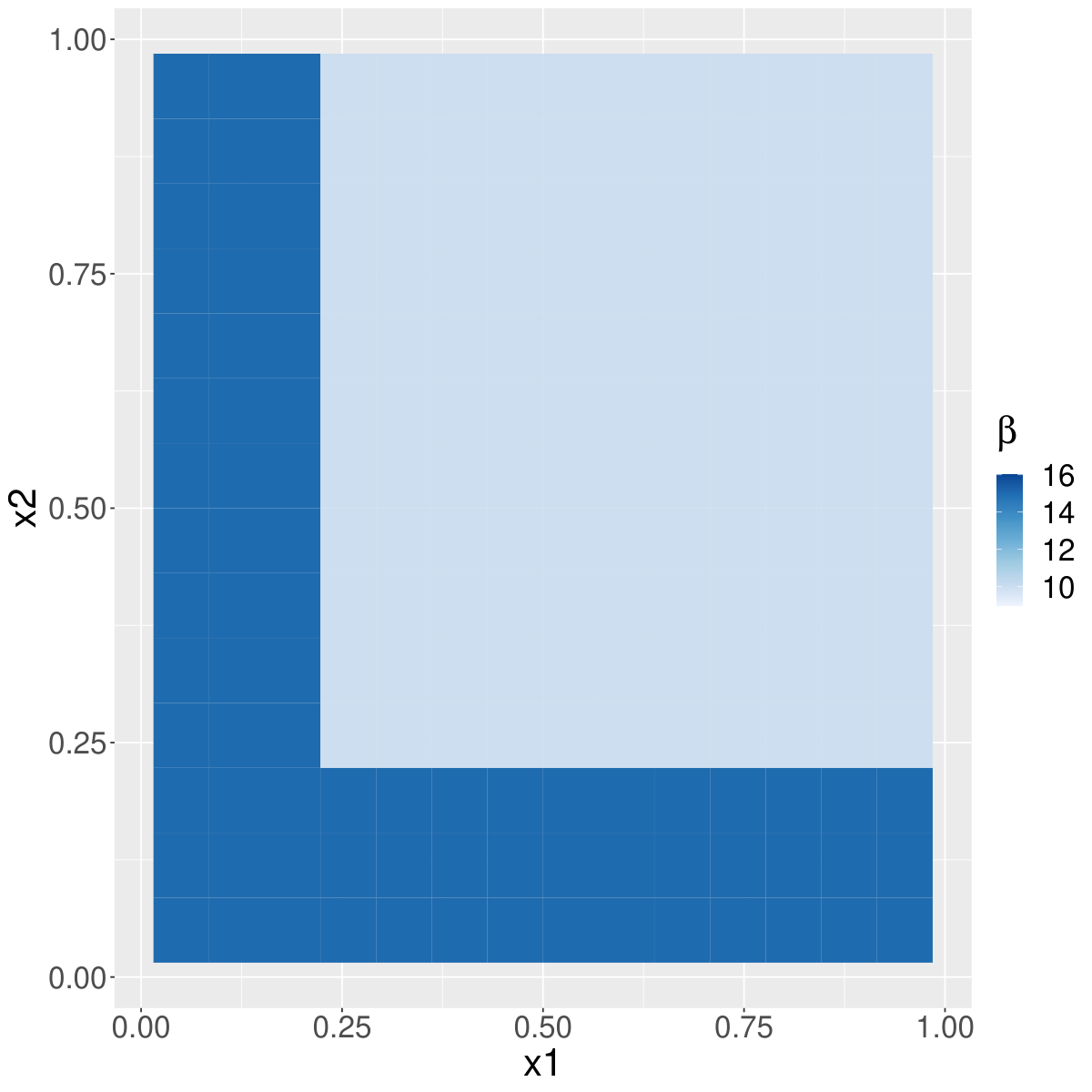
Example 2.
The predictive variable is a Bernoulli random variable with success probability , and its coefficient functions are
The error term in Model (12), , was generated by with . The modifiers were uniform random variables generated from . The censoring time was generated independently from .
Table 2 summarizes the simulation results of Scenario 2 at sample sizes at and . In this simple scenario, the conditional quantile is a piece-wise constant function. The estimation performance of by HCQRF is close to but slightly worse than that of CQRF, while the estimation of by HCQRF outperforms the one of CQRF. With the complete data, the estimation performance of HCQRF-c is always better than the one of grf-c. In some cases, grf-c is even worse than HCQRF with the censored data, especially for . Figure 2 presents the heat maps for both true and estimated quantile coefficient (averaged over Monte Carlo repetitions). It is clear that HCQRF-c does the best job of capturing the true function, followed by HCQRF and CQRF. It suggests the need of incorporating into the splittings in the presence of heterogeneous treatment effects. The post-construction weighted adjustment (as in CQRF and grf-c) alone is insufficient to restore the coefficient function. As expected, Table 2 also shows that the measurements of the estimation performance diminish with the increase of the sample size.
| Method | |||||
|---|---|---|---|---|---|
| MSE | HCQRF | 0.005 | 0.213 | 0.004 | 0.009 |
| CQRF | 0.002 | 4.140 | 0.002 | 1.907 | |
| HCQRF-c | 0.004 | 0.040 | 0.003 | 0.007 | |
| grf-c | 0.001 | 6.194 | 0.001 | 5.661 | |
| MAE | HCQRF | 0.056 | 0.134 | 0.049 | 0.074 |
| CQRF | 0.039 | 0.970 | 0.034 | 0.482 | |
| HCQRF-c | 0.053 | 0.083 | 0.046 | 0.065 | |
| grf-c | 0.028 | 1.412 | 0.023 | 1.303 | |
- •
MSE: mean squared error, MAE: mean absolute error.


Example 3.
Both and were generated randomly from . The coefficient functions (see Figure 3) are
The error term was generated with . Both the predictive variables and the modifiers were uniform random variables generated from . The censoring time was generated from .
Since are continuous in Scenario 3, CQRF can no longer be applied to estimate . We will only compare HCQRF with HCQRF-c and grf-c in this subsection. In later Section 5.4, we will compare HCQRF with CQRF in estimating the conditional quantile function under all the scenarios. The MSE and MAE of the estimated from HCQRF, HCQRF-c and grf-c are presented in Table 3. Comparing HCQRF-c and grf-c applied to the complete data, we observe that HCQRF-c have smaller MSE and MAE than grf-c for slope estimations (, and ), while the two methods produce similar results in . As expected, HCQRF is slightly worse than its benchmark HCQRF-c, and such difference diminishes with the increase of the sample size. In the meantime, HCQRF-c performs better than grf-c in all the slope estimations. Figure 3 shows the heat maps for both true and estimated quantile coefficients in a grid view of and based on 500 Monte Carlo repetitions. The figure further confirms that the proposed HCQRF approach could effectively capture the complex heterogeneous treatment effect.
[!ht]
| Method | |||||||||
|---|---|---|---|---|---|---|---|---|---|
| MSE | HCQRF | 0.028 | 0.123 | 3.990 | 2.093 | 0.017 | 0.082 | 2.755 | 1.443 |
| HCQRF-c | 0.022 | 0.105 | 3.602 | 1.884 | 0.013 | 0.069 | 2.482 | 1.295 | |
| grf-c | 0.011 | 0.181 | 8.229 | 4.239 | 0.006 | 0.172 | 8.101 | 4.176 | |
| MAE | HCQRF | 0.117 | 0.204 | 0.800 | 0.587 | 0.093 | 0.159 | 0.575 | 0.427 |
| HCQRF-c | 0.106 | 0.183 | 0.714 | 0.527 | 0.084 | 0.142 | 0.511 | 0.381 | |
| grf-c | 0.075 | 0.240 | 1.400 | 0.998 | 0.056 | 0.225 | 1.373 | 0.978 | |
- •
MSE: mean squared error, MAE: mean absolute error


Example 4.
Both and were generated randomly from independently. The coefficient functions (see the first row in Figure 4) are
The error term was generated from and the censoring time was generated from .
The simulation results are summarized in Table 4, where HCQRF-c outperforms grf-c in estimating the quantile coefficient functions, and the estimation performance of HCQRF applied to the censored data is close to the benchmark HCQRF-c. We also demonstrate the average estimation of the coefficient function by different approaches in Figure 4.
| Method | |||||||
| MSE | HCQRF | 0.977 | 1.106 | 0.694 | 0.666 | 0.814 | 0.552 |
| HCQRF-c | 0.831 | 0.778 | 0.571 | 0.577 | 0.585 | 0.454 | |
| grf-c | 2.120 | 1.336 | 0.725 | 1.110 | 1.016 | 0.565 | |
| MAE | HCQRF | 0.769 | 0.811 | 0.628 | 0.632 | 0.707 | 0.563 |
| HCQRF-c | 0.718 | 0.685 | 0.568 | 0.592 | 0.606 | 0.509 | |
| grf-c | 1.154 | 0.866 | 0.690 | 0.819 | 0.772 | 0.603 | |
| MSE: mean squared error, MAE: mean absolute error | |||||||
5.3 Sensitivity Analysis
Under a set of modified Scenario 4 specified as below, we also investigate the estimation performance under various error distributions and censoring mechanisms (completely random vs. covariate-dependent), and also investigated estimation consistency across different quantile levels (see Supplementary Materials).
-
Scenario 4a (Heterogeneous error term): The error term was generated from , where . The censoring time was generated from resulting in about censoring.
-
Scenario 4b (Heavy-tailed error term): The error term was generated from a distribution with 2 degrees of freedom. The censoring time was generated from resulting in about censoring.
-
Scenario 4c (Covariate-Dependent Censoring): The censoring time was generated by
where , resulting in about censoring.
Table 5 summarizes the resulting estimation accuracy under the modified Scenario 4, which are consistent with earlier findings. It suggests that the proposed HCQRF yields robust and stable estimations across various situations. In Supplementary Materials, we also present a modified setting in which quantile coefficient functions vary across quantile levels. Again, the proposed HCQRF delivers accurate estimations, and demonstrates advantages over other approaches.
| Scenario | Method | |||||||
| 4a | MSE | HCQRF | 0.771 | 1.052 | 0.678 | 0.458 | 0.658 | 0.430 |
| HCQRF-c | 0.638 | 0.752 | 0.541 | 0.391 | 0.471 | 0.347 | ||
| grf-c | 1.588 | 1.268 | 0.706 | 1.009 | 0.846 | 0.496 | ||
| MAE | HCQRF | 0.663 | 0.795 | 0.627 | 0.518 | 0.635 | 0.493 | |
| HCQRF-c | 0.612 | 0.677 | 0.559 | 0.482 | 0.541 | 0.443 | ||
| grf-c | 0.973 | 0.846 | 0.684 | 0.773 | 0.704 | 0.570 | ||
| 4b | MSE | HCQRF | 1.370 | 1.487 | 1.008 | 0.906 | 0.965 | 0.691 |
| HCQRF-c | 1.162 | 1.070 | 0.825 | 0.779 | 0.705 | 0.563 | ||
| grf-c | 1.921 | 1.639 | 0.863 | 1.230 | 1.080 | 0.622 | ||
| MAE | HCQRF | 0.896 | 0.948 | 0.772 | 0.732 | 0.771 | 0.630 | |
| HCQRF-c | 0.834 | 0.811 | 0.699 | 0.686 | 0.666 | 0.571 | ||
| grf-c | 1.080 | 0.965 | 0.749 | 0.863 | 0.796 | 0.634 | ||
| 4c | MSE | HCQRF | 0.977 | 1.095 | 0.683 | 0.655 | 0.686 | 0.435 |
| HCQRF-c | 0.829 | 0.804 | 0.561 | 0.578 | 0.509 | 0.359 | ||
| grf-c | 2.324 | 1.435 | 0.736 | 1.622 | 0.971 | 0.520 | ||
| MAE | HCQRF | 0.773 | 0.811 | 0.617 | 0.653 | 0.643 | 0.483 | |
| HCQRF-c | 0.724 | 0.696 | 0.555 | 0.622 | 0.555 | 0.437 | ||
| grf-c | 1.222 | 0.894 | 0.693 | 1.038 | 0.750 | 0.575 | ||
| MSE: mean squared error, MAE: mean absolute error | ||||||||
5.4 Comparing HCQRF and CQRF in Estimating the Conditional Quantiles
As mentioned in the earlier section, CQRF cannot be directly applied to estimate the coefficient function unless the is binary. However, we can estimate the conditional quantile function of given from HCQRF by
where is the estimated coefficient at by HCQRF. Hence, we compared the accuracy of the estimated from the HCQRF and CQRF under the outlined scenarios above with continuous . The resulting MSE and MAE are reported in Table 6. The HCQRF outperforms the CQRF in all the simulation scenarios, and demonstrated robust performances under the complex settings Scenario 4a, b, c.
| Scenario | Method | |||||
|---|---|---|---|---|---|---|
| MSE | MAE | MSE | MAE | |||
| 3 | 0.5 | HCQRF | 0.531 | 0.262 | 0.373 | 0.194 |
| CQRF | 3.994 | 1.626 | 4.001 | 1.631 | ||
| 4 | 0.5 | HCQRF | 2.076 | 1.098 | 1.424 | 0.899 |
| CQRF | 29.25 | 4.185 | 29.194 | 4.172 | ||
| 4a | 0.5 | HCQRF | 1.834 | 1.012 | 1.160 | 0.805 |
| CQRF | 28.805 | 4.155 | 28.262 | 4.114 | ||
| 4b | 0.5 | HCQRF | 2.516 | 1.196 | 1.639 | 0.968 |
| CQRF | 30.138 | 4.236 | 29.226 | 4.173 | ||
| 4c | 0.5 | HCQRF | 2.144 | 1.121 | 1.465 | 0.932 |
| CQRF | 29.972 | 4.233 | 29.598 | 4.204 | ||
| 6 | 0.25 | HCQRF | 2.453 | 1.213 | 1.713 | 1.026 |
| CQRF | 30.036 | 4.243 | 29.629 | 4.208 | ||
| 6 | 0.5 | HCQRF | 2.186 | 1.137 | 1.520 | 0.956 |
| CQRF | 30.14 | 4.25 | 29.779 | 4.219 | ||
| 6 | 0.75 | HCQRF | 2.208 | 1.116 | 1.475 | 0.918 |
| CQRF | 30.445 | 4.275 | 30.058 | 4.244 | ||
- •
MSE: mean squared error, MAE: mean absolute error
5.5 Variable Importance
In this subsection, we examine the variable importance decomposition proposed in Section 4.2 using Scenario 2, where the predictive variable is a binary variable. In Scenario 2, is a constant and depends on and . The result of the variable importance decomposition based on Scenario 2 is reported in Figure 5 at . In the results, we demonstrate the importance score of by . Figure 5 clearly shows that the importance scores of and are close to 0 for while they are away from 0 for . The importance plots show that the proposed variable importance decomposition distinguishes the different dependence structures of and .
6 Real Data
We applied both HCQRF and CQRF to a randomized phase III clinical trial which aims to compare the efficacy of fluorouracil, leucovorin, and irinotecan (FOLFIRI) alone versus panitumumab plus FOLFIRI in patients who were previously treated for metastatic colorectal cancer (Peeters et al. 2014). In this trial, patients were randomly assigned to one of the two treatments, panitumumab plus FOLFIRI or FOLFIRI alone. The primary endpoint is progression-free survival (PFS). Besides estimating their treatment effects on PFS, we are also interested in identifying patient characteristics that maybe modify the treatment effects. Such knowledge help design more targeted treatment plans to improve outcomes.
The study sample includes 830 patients, among those, 783 patients progressed after their treatments (i.e., PFS observed). The main variable of interest is the treatment assignment (FOLFIRI alone = 0, Panitumumab + FOLFIRI = 1). The FOLFIRI-alone arm consists of 413 patients while the panitumumab plus FOLFIRI arm has 417 patients. We also consider ten covariates as potential effect modifiers, including age (in years) and lactate dehydrogenase value at baseline (LDH, upper limit of normal), prior mCRC Bevacizumab use (yes = 1, no = 0), prior mCRC Oxaliplatin Exposure (yes = 1, no = 0), KRAS (wild-type = 1, mutant = 2), prim tumor type (rectum = 0, colon = 1), sex (male = 0, female = 1), race (white or Caucasian = 1, others = 0), the number of baseline metastatic sites (from 1 to 8), and eastern cooperative oncology group at baseline (ECOG,0, 1, and ). We randomly split the data into a training set with 80% data points(n = 664), and a test set with the remaining 166 observations. We construct both HCQRF and CQRF from the training data, following the outlined algorithms in Section 4.3. The hyperparameters in the forest models are the same as the specifications in Section 4.4.
6.1 Variable Importance
We calculate the variable importance from the constructed HCQRF and CQRF, respectively. For HCQRF, we follow the algorithm in Section 4.2 to calculate the variable importance (VI) with permutations, and future decompose the total VI into VI for (main effect) and VI for (interactive effects). We note that VI of CQRF was not officially developed in Li and Bradic 2020. As CQRF follows the scheme of generalized random forest (Athey et al. 2019), we apply the default variable importance in the grf package (Tibshirani et al. 2022), which is a weighted sum of how many times a variable was split at each depth in the forest. We set the maximal depth to be 4.
The resulting variable importance from HCQRF and CQRF are presented in Figure 6 and Figure 7 respectively. The first column in Figure 6 presents the total VI at three quantile levels (0.25, 0.5, and 0.75). Top-ranked variables include ECOG, prior Oxalilatin exposure, LDH value, which are consistent with the literature (Cohen et al. 2009; Li et al. 2016). The second and the third columns in in Figure 6 present the VI for and correspondingly. One interesting observation is the importance of KRAS mutation. KRAS is a group of genes involved in the epidermal growth factor receptor pathway. The importance of KRAS is among the middle to lower ranks for the overall importance and effect of . However, it is ranked at the top when it comes to its importance for . It suggests that KRAS mutation may not affect the disease progress on its own, but could modify the treatment effect on PFS, which is consistent with the literature reports. For example, (Peeters et al. 2014) reported that KRAS mutations predicts the efficacy of anti-epidermal growth factor receptor therapies, including panitumumab, and hence they may modify the treatment effect. The variable importance reported from CQRF (as in Figure 7) are similar to the overall importance of HCQRF and does not recognize the importance of KRAS.
6.2 Estimated Quantile Treatment Effect
Since KRAS is identified as a top-ranked effect modifier of the treatment effect, we stratify the estimation of quantile treatment effect (QTE) by KRAS types. In HCQRF, the estimated represents the individualized QTE. In CQRF, we estimate individualized QTE for each observation in the test set by . Figure 8 demonstrates the box plots of the individualized QTE stratified by the two KRAS types at quantile level . The results based on HCQRF clearly manifest that the individualized treatment effects are different between the two KRAS types. However, such differences based on CQRF are less evident. The top panel of Table 7 displays the average quantile treatment effect (AQTE) from HCQRF and CQRF stratified by KRAS types. CQRF reports comparable treatment effects, while HCQRF suggests very different treatment effects by the KRAS mutation status, across all the quantile levels.
6.3 Empirical Validation
The estimates from CQRF and HCQF disagree on the existence of KRAS-treatment interaction. In this subsection, we conduct an empirical validation. We stratify the sample by treatment assignment and KRAS status (229 patients with wild-type KRAS and 184 patients with mutant KRAS taking FOLIFIRI alone; 234 patients with wild-type KRAS and 183 patients with mutant KRAS taking Panitumumab plus FOLFIRI) and construct Kaplan-Meier survival functions of PFS within each stratum. The estimated Kaplan-Meier curves in Figure 9 display a noticeably larger difference in PFS between the two treatment arms among the patients with wild-type KRAS. As KS estimation is model-free, we view the agreement with KS estimation as the indication of a good fit to the data. To quantify such agreement, we also measure the distance between the KS-estimated quantile function and the model-derived conditional quantiles from CQRF and HCQRF. For each observation , we calculates its conditional quantiles at , and use linear interpolations to construction for any . Since KS-estimates are marginal quantile functions in each stratum, while are conditional quantiles, they are not directly comparable. To assess their agreement, we calculate
where is the distribution function induced from the conditional quantile function , and is KS-estimated stratum-specific th quantile. If the model fits the data well, we expect the resulting to be equal to its nominal level . The bottom half of Table 7 lists the at quantile levels in each stratum (i.e., and ). Clearly, the ones derived from HCQRF are consistently closer to their nominal level . We conclude that there is empirical evidence supporting the KRAS-treatment interaction.
| KRAS = wild-type | KRAS = mutant | |||||||
|---|---|---|---|---|---|---|---|---|
| AQTE | HCQRF | 30.788 | 61.584 | 82.529 | 1.681 | 13.469 | 44.617 | |
| CQRF | 8.502 | 12.918 | 27.088 | 5.973 | 7.716 | 18.070 | ||
| HCQRF | treatment | 0.278 | 0.503 | 0.729 | 0.228 | 0.503 | 0.716 | |
| control | 0.251 | 0.484 | 0.765 | 0.237 | 0.538 | 0.748 | ||
| CQRF | treatment | 0.325 | 0.558 | 0.779 | 0.224 | 0.497 | 0.728 | |
| control | 0.211 | 0.421 | 0.725 | 0.233 | 0.517 | 0.719 | ||
In the analysis of the randomized clinical trial data, KRAS is identified as a top-ranked important variable of the treatment effect through the proposed variable importance decomposition. In contrast, the ranking of the importance in CQRF does not demonstrate a similar result. Additional comparisons of the individualized QTE and AQTE between HCQRF and CQRF confirm our conclusion from the variable importance. Moreover, the result of the empirical validation also shows that the estimation obtained by HCQRF is more congruent with the data.
7 Discussion
In this paper, we develop a hybrid censored quantile regression forest to assess the heterogeneous quantile effects of censored data. The proposed estimation procedure takes advantage of both random forest and censored quantile regression. We also develop a variable importance decomposition to measure the impact of a modifier only on the treatment effect if the predictive variable is binary. Both the simulation studies and the real data analysis demonstrate that the proposed approach can achieve a better estimation performance and insightful variable importance results.
In Section 4.2, we assume that the treatments are randomly assigned, and the method can be easily extended to handle the case where the treatments assignments satisfy the ignorability assumptions (Rosenbaum and Rubin 1983). Specifically, we replace the term in (11) by a weight if or if , where is an estimated probability of given and can be estimated by a logistic regression model.
Based on the simulation studies and real data analysis, the proposed HCQRF provides a good estimation of the coefficient function as well as an insightful variable ranking. In this paper, we focus on the case of a finite number of predictive variables. One promising future work is to extend the proposed approach to high-dimensional predictors. Constructing the confidence interval of the estimated coefficient is also one of the promising future research. The bootstrap of little bags technique used in grf (Athey et al. 2019) may help us to quantify the uncertainty of the estimate by our proposed approach.
acknowledgments-disclosure-of-funding.
This is partially supported by NSF/NIH (DMS-1953527), NIH (R21HL156288), and Direct Grants for the Chinese University of Hong Kong (171428926).References
- Athey et al. (2019) Susan Athey, Julie Tibshirani, Stefan Wager, et al. Generalized random forests. The Annals of Statistics, 47(2):1148–1178, 2019.
- Breiman (2001) Leo Breiman. Random forests. Machine learning, 45(1):5–32, 2001.
- Cai and Xu (2009) Zongwu Cai and Xiaoping Xu. Nonparametric quantile estimations for dynamic smooth coefficient models. Journal of the American Statistical Association, 104(485):371–383, 2009.
- Cohen et al. (2009) SJ Cohen, CJA Punt, N Iannotti, BH Saidman, KD Sabbath, NY Gabrail, Joel Picus, MA Morse, E Mitchell, MC Miller, et al. Prognostic significance of circulating tumor cells in patients with metastatic colorectal cancer. Annals of oncology, 20(7):1223–1229, 2009.
- De Backer et al. (2019) Mickaël De Backer, Anouar El Ghouch, and Ingrid Van Keilegom. An adapted loss function for censored quantile regression. Journal of the American Statistical Association, 114(527):1126–1137, 2019.
- Hájek (1965) Jaroslav Hájek. Extension of the kolmogorov-smirnov test to regression alternatives. In Bernoulli 1713 Bayes 1763 Laplace 1813, pages 45–60. Springer, 1965.
- Hastie and Tibshirani (1993) Trevor Hastie and Robert Tibshirani. Varying-coefficient models. Journal of the Royal Statistical Society: Series B (Methodological), 55(4):757–779, 1993.
- Honda (2004) Toshio Honda. Quantile regression in varying coefficient models. Journal of statistical planning and inference, 121(1):113–125, 2004.
- Hothorn et al. (2006) Torsten Hothorn, Peter Bühlmann, Sandrine Dudoit, Annette Molinaro, and Mark J Van Der Laan. Survival ensembles. Biostatistics, 7(3):355–373, 2006.
- Huang et al. (2002) Jianhua Z Huang, Colin O Wu, and Lan Zhou. Varying-coefficient models and basis function approximations for the analysis of repeated measurements. Biometrika, 89(1):111–128, 2002.
- Ishwaran et al. (2008) Hemant Ishwaran, Udaya B Kogalur, Eugene H Blackstone, Michael S Lauer, et al. Random survival forests. The Annals of Applied Statistics, 2(3):841–860, 2008.
- Koenker (2005) Roger Koenker. Quantile Regression. Econometric Society Monographs. Cambridge University Press, 2005. doi: 10.1017/CBO9780511754098.
- Kosorok and Moodie (2015) Michael R Kosorok and Erica EM Moodie. Adaptive treatment strategies in practice: planning trials and analyzing data for personalized medicine. SIAM, 2015.
- Kravitz et al. (2004) Richard L Kravitz, Naihua Duan, and Joel Braslow. Evidence-based medicine, heterogeneity of treatment effects, and the trouble with averages. The Milbank Quarterly, 82(4):661–687, 2004.
- Leng et al. (2013) Chenlei Leng, Xingwei Tong, et al. A quantile regression estimator for censored data. Bernoulli, 19(1):344–361, 2013.
- Li and Bradic (2020) Alexander Hanbo Li and Jelena Bradic. Censored quantile regression forest. In International Conference on Artificial Intelligence and Statistics, pages 2109–2119, 2020.
- Li et al. (2016) Guanghua Li, Zhao Wang, Jianbo Xu, Hui Wu, Shirong Cai, and Yulong He. The prognostic value of lactate dehydrogenase levels in colorectal cancer: a meta-analysis. BMC cancer, 16(1):1–9, 2016.
- Lin and Jeon (2006) Yi Lin and Yongho Jeon. Random forests and adaptive nearest neighbors. Journal of the American Statistical Association, 101(474):578–590, 2006.
- Loh (2002) Wei-Yin Loh. Regression trees with unbiased variable selection and interaction detection. Statistica sinica, pages 361–386, 2002.
- Loh (2014) Wei-Yin Loh. Fifty years of classification and regression trees. International Statistical Review, 82(3):329–348, 2014.
- McKeague et al. (2001) Ian W McKeague, Sundarraman Subramanian, and Yanqing Sun. Median regression and the missing information principle. Journal of nonparametric statistics, 13(5):709–727, 2001.
- Meinshausen (2006) Nicolai Meinshausen. Quantile regression forests. Journal of Machine Learning Research., 7:983–999, 2006.
- Peeters et al. (2014) Marc Peeters, TJ Price, A Cervantes, AF Sobrero, M Ducreux, Y Hotko, T André, E Chan, F Lordick, CJA Punt, et al. Final results from a randomized phase 3 study of folfiripanitumumab for second-line treatment of metastatic colorectal cancer. Annals of Oncology, 25(1):107–116, 2014.
- Peng and Huang (2008) Limin Peng and Yijian Huang. Survival analysis with quantile regression models. Journal of the American Statistical Association, 103(482):637–649, 2008.
- Portnoy (2003) Stephen Portnoy. Censored regression quantiles. Journal of the American Statistical Association, 98(464):1001–1012, 2003.
- Powell (1984) James L Powell. Least absolute deviations estimation for the censored regression model. Journal of Econometrics, 25(3):303–325, 1984.
- Powell (1986) James L Powell. Censored regression quantiles. Journal of Econometrics, 32(1):143–155, 1986.
- Rosenbaum and Rubin (1983) Paul R Rosenbaum and Donald B Rubin. The central role of the propensity score in observational studies for causal effects. Biometrika, 70(1):41–55, 1983.
- Scornet (2016) Erwan Scornet. Random forests and kernel methods. IEEE Transactions on Information Theory, 62(3):1485–1500, 2016.
- Steingrimsson et al. (2019) Jon Arni Steingrimsson, Liqun Diao, and Robert L Strawderman. Censoring unbiased regression trees and ensembles. Journal of the American Statistical Association, 114(525):370–383, 2019.
- Sun (2020) Yuan Sun. On Rank-Based Inference for Quantile Regression. PhD thesis, The University of Michigan, 2020.
- Tibshirani et al. (2022) Julie Tibshirani, Susan Athey, Erik Sverdrup, and Stefan Wager. grf: Generalized Random Forests, 2022. URL https://CRAN.R-project.org/package=grf. R package version 2.1.0.
- Wang and Wang (2009) Huixia Judy Wang and Lan Wang. Locally weighted censored quantile regression. Journal of the American Statistical Association, 104(487):1117–1128, 2009.
- Wang et al. (2013) Huixia Judy Wang, Jianhui Zhou, and Yi Li. Variable selection for censored quantile regresion. Statistica Sinica, 23(1):145, 2013.
- Xie et al. (2015) Shangyu Xie, Alan TK Wan, and Yong Zhou. Quantile regression methods with varying-coefficient models for censored data. Computational Statistics & Data Analysis, 88:154–172, 2015.
- Zhu and Kosorok (2012) Ruoqing Zhu and Michael R Kosorok. Recursively imputed survival trees. Journal of the American Statistical Association, 107(497):331–340, 2012.
Supplementary Materials of ”Hybrid Censored Quantile Regression Forest to Assess the Heterogeneous Effects”
A Extra Simulation Results
| Method | |||||
|---|---|---|---|---|---|
| Relative MSE | HCQRF | 1.9e-04 | 0.001 | 1.5e-04 | 6.1e-05 |
| CQRF | 9.6e-05 | 0.018 | 7.1e-05 | 0.008 | |
| HCQRF-c | 1.7e-04 | 0.000 | 1.4e-04 | 4.9e-05 | |
| grf-c | 5.0e-05 | 0.028 | 3.4e-05 | 0.025 | |
| Relative MAE | HCQRF | 0.011 | 0.011 | 0.010 | 0.006 |
| CQRF | 0.008 | 0.067 | 0.007 | 0.033 | |
| HCQRF-c | 0.011 | 0.007 | 0.009 | 0.006 | |
| grf-c | 0.006 | 0.097 | 0.005 | 0.089 | |
- •
MSE: mean squared error, MAE: mean absolute error.
| Method | |||||||||
|---|---|---|---|---|---|---|---|---|---|
| Relative MSE | HCQRF | 0.001 | -a | 0.112 | - | 0.001 | - | 0.086 | - |
| HCQRF-c | 0.001 | - | 0.104 | - | 0.001 | - | 0.078 | - | |
| grf-c | 4E-4 | - | 0.088 | - | 2E-4 | - | 0.086 | - | |
| Relative MAE | HCQRF | 0.023 | - | 0.136 | - | 0.019 | - | 0.102 | - |
| HCQRF-c | 0.021 | - | 0.122 | - | 0.017 | - | 0.091 | - | |
| grf-c | 0.015 | - | 0.180 | - | 0.011 | - | 0.174 | - | |
- •
MSE: mean squared error, MAE: mean absolute error
- •
a: relative evaluation measurements are unavailable for because .
| Method | |||||||
| Relative MSE | HCQRF | 0.132 | 0.061 | 0.037 | 0.095 | 0.047 | 0.030 |
| HCQRF-c | 0.112 | 0.043 | 0.030 | 0.083 | 0.033 | 0.025 | |
| grf-c | 0.284 | 0.075 | 0.038 | 0.160 | 0.058 | 0.031 | |
| Relative MAE | HCQRF | 0.244 | 0.169 | 0.142 | 0.203 | 0.149 | 0.128 |
| HCQRF-c | 0.227 | 0.143 | 0.128 | 0.191 | 0.128 | 0.116 | |
| grf-c | 0.365 | 0.181 | 0.156 | 0.264 | 0.163 | 0.137 | |
| MSE: mean squared error, MAE: mean absolute error | |||||||
| Scenario | Method | |||||||
| 4a | Relative MSE | HCQRF | 0.105 | 0.044 | 0.045 | 0.075 | 0.033 | 0.029 |
| HCQRF-c | 0.087 | 0.037 | 0.037 | 0.063 | 0.027 | 0.024 | ||
| grf-c | 0.214 | 0.036 | 0.042 | 0.163 | 0.026 | 0.031 | ||
| Relative MAE | HCQRF | 0.210 | 0.158 | 0.149 | 0.174 | 0.133 | 0.117 | |
| HCQRF-c | 0.193 | 0.142 | 0.134 | 0.162 | 0.120 | 0.105 | ||
| grf-c | 0.307 | 0.150 | 0.157 | 0.260 | 0.128 | 0.132 | ||
| 4b | Relative MSE | HCQRF | 0.190 | 0.090 | 0.052 | 0.123 | 0.060 | 0.036 |
| HCQRF-c | 0.162 | 0.065 | 0.043 | 0.107 | 0.044 | 0.029 | ||
| grf-c | 0.266 | 0.099 | 0.045 | 0.169 | 0.067 | 0.032 | ||
| Relative MAE | HCQRF | 0.288 | 0.205 | 0.172 | 0.234 | 0.172 | 0.141 | |
| HCQRF-c | 0.269 | 0.175 | 0.156 | 0.219 | 0.149 | 0.128 | ||
| grf-c | 0.348 | 0.209 | 0.167 | 0.276 | 0.178 | 0.142 | ||
| 4c | Relative MSE | HCQRF | 0.134 | 0.066 | 0.036 | 0.088 | 0.039 | 0.024 |
| HCQRF-c | 0.114 | 0.049 | 0.029 | 0.078 | 0.029 | 0.020 | ||
| grf-c | 0.321 | 0.086 | 0.039 | 0.218 | 0.055 | 0.029 | ||
| Relative MAE | HCQRF | 0.249 | 0.174 | 0.138 | 0.206 | 0.135 | 0.110 | |
| HCQRF-c | 0.233 | 0.150 | 0.124 | 0.196 | 0.116 | 0.100 | ||
| grf-c | 0.394 | 0.192 | 0.155 | 0.327 | 0.157 | 0.131 | ||
| MSE: mean squared error, MAE: mean absolute error | ||||||||
| Scenario | Method | |||||||
|---|---|---|---|---|---|---|---|---|
| MSE | RMSE | RMAE | MSE | RMSE | RMAE | |||
| 2 | 0.5 | HCQRF | 0.428 | 0.003 | 0.013 | 0.112 | 0.001 | 0.007 |
| CQRF | 0.287 | 0.002 | 0.011 | 0.056 | 3E-4 | 0.005 | ||
| 3 | 0.5 | HCQRF | 0.531 | 0.004 | 0.024 | 0.373 | 0.003 | 0.018 |
| CQRF | 3.994 | 0.042 | 0.168 | 4.001 | 0.040 | 0.165 | ||
| 4 | 0.5 | HCQRF | 2.076 | 0.015 | 0.081 | 1.424 | 0.015 | 0.073 |
| CQRF | 29.250 | 0.224 | 0.310 | 29.194 | 0.298 | 0.339 | ||
| 4a | 0.5 | HCQRF | 1.834 | 0.013 | 0.074 | 1.160 | 0.009 | 0.061 |
| CQRF | 28.805 | 0.112 | 0.263 | 28.262 | 0.112 | 0.262 | ||
| 4b | 0.5 | HCQRF | 2.516 | 0.021 | 0.091 | 1.639 | 0.016 | 0.078 |
| CQRF | 30.138 | 0.246 | 0.323 | 29.226 | 0.286 | 0.335 | ||
| 4c | 0.5 | HCQRF | 2.144 | 0.019 | 0.086 | 1.465 | 0.014 | 0.073 |
| CQRF | 29.972 | 0.268 | 0.327 | 29.598 | 0.278 | 0.327 | ||
| 6 | 0.25 | HCQRF | 2.453 | 0.022 | 0.094 | 1.713 | 0.016 | 0.080 |
| CQRF | 30.036 | 0.266 | 0.328 | 29.629 | 0.277 | 0.327 | ||
| 6 | 0.5 | HCQRF | 2.186 | 0.019 | 0.087 | 1.520 | 0.014 | 0.074 |
| CQRF | 30.14 | 0.266 | 0.327 | 29.779 | 0.278 | 0.327 | ||
| 6 | 0.75 | HCQRF | 2.208 | 0.019 | 0.085 | 1.475 | 0.014 | 0.071 |
| CQRF | 30.445 | 0.266 | 0.327 | 30.058 | 0.277 | 0.327 | ||
- •
MSE: mean squared error, RMSE: relative mean squared error RMAE: relative mean absolute error
B Extra Simulations
Example 5.
We generated data from the model (12) with , and . The predictive variable and the modifiers were generated from . The censoring time was generated from , resulting in censoring. The set of modifiers were generated randomly from and .
In Scenario 5, the coefficient functions are constants. Censored quantile regression (cqr, Wang and Wang 2009) can also be applied to this scenario. Thus, we compare the estimation performance of HCQRF and cqr in Scenario 5. When the quatile coefficients are constants, censored quantile regression (cqr) achieves the optimal estimation performance. It is inefficient to apply a complex estimation framework such as random forest on the data with simple true underlying model. The result in Table S6 shows that the proposed HCQRF can still achieve a good estimation performance.
| Scenario | Method | |||||
|---|---|---|---|---|---|---|
| 5 | MSE | HCQRF | 0.302 | 0.890 | 0.114 | 0.664 |
| cqr | 0.036 | 0.111 | 0.007 | 0.069 | ||
| Relative MSE | HCQRF | 0.007 | 0.009 | 0.003 | 0.007 | |
| cqr | 0.002 | 0.001 | 0.001 | 0.000 | ||
| Relative MAE | HCQRF | 0.068 | 0.074 | 0.042 | 0.065 | |
| cqr | 0.041 | 0.026 | 0.027 | 0.017 | ||
- •
MSE: mean squared error, MAE: mean absolute error, cqr: censored quantile regression
In Scenario 6, we consider an extended scenario where is a coefficient function varying across different quantile levels
Example 6.
We generated data from the model (12) with
| (1) |
where is generated from a Chi-sqaured distribution with degree freedom 1. It indicates from (6) that can be rewrited as a function depending on both and quantile level , , where is the th quantile of . The predictive variables and the modifiers were randomly generated from independently. The error term was generated from . The censoring time was generated from . The set of modifiers were generated randomly from and .
Table S8 summarizes the simulation results of Scenario 6 at quantile levels . Table 6 summarizes the estimation performance of the conditional quantile for the four different extended scenarios.
| Method | ||||||||
| Relative MSE | HCQRF | 0.162 | 0.067 | 0.037 | 0.110 | 0.041 | 0.027 | |
| HCQRF-c | 0.112 | 0.050 | 0.027 | 0.080 | 0.030 | 0.020 | ||
| grf-c | 0.327 | 0.082 | 0.035 | 0.222 | 0.056 | 0.027 | ||
| Relative MAE | HCQRF | 0.274 | 0.175 | 0.140 | 0.228 | 0.138 | 0.118 | |
| HCQRF-c | 0.233 | 0.149 | 0.120 | 0.198 | 0.118 | 0.099 | ||
| grf-c | 0.398 | 0.186 | 0.145 | 0.329 | 0.158 | 0.123 | ||
| Relative MSE | HCQRF | 0.136 | 0.066 | 0.036 | 0.091 | 0.040 | 0.024 | |
| HCQRF-c | 0.118 | 0.050 | 0.030 | 0.080 | 0.030 | 0.020 | ||
| grf-c | 0.325 | 0.087 | 0.038 | 0.222 | 0.056 | 0.028 | ||
| Relative MAE | HCQRF | 0.251 | 0.175 | 0.137 | 0.209 | 0.136 | 0.109 | |
| HCQRF-c | 0.236 | 0.152 | 0.124 | 0.198 | 0.118 | 0.099 | ||
| grf-c | 0.397 | 0.194 | 0.151 | 0.329 | 0.158 | 0.127 | ||
| Relative MSE | HCQRF | 0.141 | 0.085 | 0.035 | 0.097 | 0.055 | 0.023 | |
| HCQRF-c | 0.118 | 0.050 | 0.030 | 0.080 | 0.030 | 0.020 | ||
| grf-c | 0.325 | 0.087 | 0.041 | 0.222 | 0.056 | 0.031 | ||
| Relative MAE | HCQRF | 0.258 | 0.193 | 0.138 | 0.217 | 0.155 | 0.111 | |
| HCQRF-c | 0.236 | 0.152 | 0.126 | 0.198 | 0.118 | 0.101 | ||
| grf-c | 0.397 | 0.194 | 0.160 | 0.329 | 0.158 | 0.137 | ||
| MSE: mean squared error, MAE: mean absolute error | ||||||||
| Method | ||||||||
| MSE | HCQRF | 1.190 | 1.073 | 0.709 | 0.819 | 0.713 | 0.498 | |
| HCQRF-c | 0.823 | 0.796 | 0.523 | 0.593 | 0.527 | 0.359 | ||
| grf-c | 2.364 | 1.283 | 0.662 | 1.648 | 0.981 | 0.488 | ||
| MAE | HCQRF | 0.860 | 0.837 | 0.649 | 0.726 | 0.660 | 0.516 | |
| HCQRF-c | 0.734 | 0.707 | 0.556 | 0.629 | 0.565 | 0.435 | ||
| grf-c | 1.230 | 0.901 | 0.662 | 1.046 | 0.755 | 0.541” | ||
| MSE | HCQRF | 0.987 | 1.097 | 0.691 | 0.679 | 0.701 | 0.435 | |
| HCQRF-c | 0.856 | 0.833 | 0.575 | 0.593 | 0.527 | 0.359 | ||
| grf-c | 2.356 | 1.452 | 0.732 | 1.648 | 0.981 | 0.510 | ||
| MAE | HCQRF | 0.779 | 0.810 | 0.617 | 0.663 | 0.651 | 0.483 | |
| HCQRF-c | 0.734 | 0.707 | 0.560 | 0.629 | 0.565 | 0.435 | ||
| grf-c | 1.230 | 0.901 | 0.682 | 1.046 | 0.755 | 0.560 | ||
| MSE | HCQRF | 1.021 | 1.414 | 0.697 | 0.715 | 0.955 | 0.439 | |
| HCQRF-c | 0.856 | 0.833 | 0.601 | 0.593 | 0.527 | 0.375 | ||
| grf-c | 2.356 | 1.452 | 0.818 | 1.648 | 0.981 | 0.580 | ||
| MAE | HCQRF | 0.798 | 0.897 | 0.634 | 0.689 | 0.740 | 0.499 | |
| HCQRF-c | 0.734 | 0.707 | 0.580 | 0.629 | 0.565 | 0.452 | ||
| grf-c | 1.230 | 0.901 | 0.736 | 1.046 | 0.755 | 0.614 | ||
| MSE: mean squared error, MAE: mean absolute error | ||||||||